


Classic theories of democracy as well as contemporary theories of voting behavior and political representation hold that voters assess politicians on the basis of their positions on issues of the day (Downs Reference Downs1957; Key Reference Key1966). Candidates and parties announce positions on issues in order to win votes, and voters choose the alternatives that best represent their interests on those issues. Legislators and executives who are out of step with their constituents are voted out of office (e.g., Erikson and Wright Reference Erikson, Wright, Dodd and Oppenheimer1993; Canes-Wrone et al. Reference Canes-Wrone, Brady and Cogan2002). These assumptions undergird centuries of democratic theory and decades of spatial modeling.
This portrait of electoral politics, however, runs counter to much of American survey research over the last six decades. Converse (Reference Converse and Apter1964) issued the most stunning and most frequently cited critique. He found that voters exhibit little consistency in their attitudes over time and little ideological constraint from one issue to the next. Accordingly, the conventional wisdom portrayed in most American politics textbooks is that the vast majority of American voters do not have coherent issue preferences or even attitudes (e.g., Fiorina and Peterson Reference Fiorina and Peterson1998, 144–52). In his comprehensive literature review, Kinder (Reference Kinder1998, 796) wrote: “Precious few Americans make sophisticated use of political abstractions. Most are mystified by or at least indifferent to standard ideological concepts, and not many express consistently liberal, conservative, or centrist positions on government policy.”
This paper argues that such conclusions are driven largely by measurement error associated with the analysis of individual survey items. We revisit the American National Election Study panels with a relatively simple, transparent, and old-fashioned approach to reducing measurement error. We show that issue scales composed of multiple measures are much more stable than individual survey items and, with enough questions, can even approach the stability of party identification.
Following from the apparent incoherence and instability of voters' preferences, the conventional wisdom also holds that preferences over public policy issues have little independent impact on citizens' voting decisions. Yet once we implement a very simple correction for measurement error, we show that issue preferences have a large effect on voting in U.S. presidential elections, again approaching that of party identification.
Most research using individual-level survey data over the past several decades echoes the findings of The American Voter (Campbell et al. Reference Campbell, Miller, Converse and Stokes1960): voters rely on their party identification and impressions about candidate image when deciding how to vote, and ideology or opinions on specific policies play a modest role at best. Although there are certainly prominent exceptions in the literature (e.g., Green et al. 2002; Abramowitz and Saunders Reference Abramowitz and Saunders1998), these findings are recounted in many textbooks on American politics and elections. For example, Polsby and Wildavsky (Reference Polsby and Wildavsky2000, 15–17) write: “By the time we get down to those who know and care about and can discriminate between party positions on issues, we usually have a small proportion of the electorate. . . So while candidates matter sometimes and issues matter sometimes, and both are capable of affecting who wins, for most voters party matters almost all the time.”
Yet an undercurrent of survey research, at least since the 1980s, argues that it is possible to identify “core values” or “predispositions” that are coherent and stable (McClosky and Zaller Reference McClosky and Zaller1984; Feldman Reference Feldman1988; Heath et al. Reference Heath, Evans and Martin1994.) When issues are framed in terms of such core values, survey respondents readily make sense of the choices at hand (Sniderman and Piazza Reference Sniderman and Piazza1993). Further research shows that scaled values of survey responses have considerable traction in predicting party identification, candidate evaluations, and vote choice (e.g., Carmines and Stimson Reference Carmines and James1980; Miller and Shanks Reference Miller and Shanks1996; Erikson and Tedin Reference Erikson and Tedin2007). Adding to the puzzle, averaging across large numbers of individuals produces aggregate public opinion on issues that is quite stable over time and strongly associated with public policy outcomes (e.g., Page and Shapiro Reference Page and Shapiro1982; Erikson et al. Reference Erikson, MacKuen and Stimson2002).
One natural explanation for this pattern of findings is that the responses to individual issue questions in surveys are plagued with large amounts of measurement error. Measurement error in surveys arises for a variety of reasons, including vague question wordings, vague response categories or categories that do not reflect the individual's actual attitude, inattentiveness on the part of the respondent, and even typographical errors (see Mosteller Reference Mosteller, Kruskal and Tanur1968). Achen (Reference Achen1975) showed that measurement error in survey items is sufficient to explain the low correlations of individuals' issue preferences over time and the apparent lack of constraint. The correlations observed by Converse are easily reconciled with a model in which there is a high degree of measurement error and a high degree of stability in preferences (see also Erikson Reference Erikson1978, Reference Erikson1979). Mysteriously, however, this is not a dominant idea, at least not in the American context. We think it should be.
In this paper, we show that there is a large amount of measurement error in the responses to typical survey questions on policy issues, and we suggest a simple method for reducing the effects of this error. Our approach uses multiple measures. First, multiple measures allow us to estimate the relative amounts of signal and noise in survey items. Second, constructing scores by averaging several items together—either by taking the simple arithmetic mean or by using factor analysis—yields much better estimates of respondents' underlying issue preferences. Averaging multiple items reduces the variance of the measurement error at roughly the rate of one over the number of items used. The scores can then be used to study the stability of latent preferences and the extent of issue voting.
This technique is widely used in political science to construct legislative roll-call voting scores, and has been used for over 70 years in psychometrics to construct test scores (e.g., Kuder and Richardson Reference Kuder and Richardson1937; Lord and Novick Reference Lord and Novick1968). Outside the American context, Evans, Heath, and Lallje (Reference Evans, Heath and Lalljee1996) used this approach to cast doubt on Butler and Stokes's (Reference Butler and Stokes1974) claims about the instability and incoherence of political attitudes in Britain. Yet in spite of useful methodological overviews by McIver and Carmines (Reference McIver and Carmines1981) and Spector (Reference Spector1992), multiple measures are rarely used in American survey research.
A number of studies of the American public have used LISREL to estimate structural models that explicitly incorporate measurement error and use multiple survey items to help identify latent variables (e.g., Judd and Milburn Reference Judd and Milburn1980; Jackson Reference Jackson1983; Norpoth and Lodge Reference Norpoth and Milton1985; Hurwitz and Peffley Reference Hurwitz and Peffley1987; Moskowitz and Jenkins Reference Moskowitz and Jenkins2004). Virtually all of these papers demonstrate that the amount of measurement error in most survey items is large, and after correcting for this, the latent variables are highly stable over time. Yet such studies—harshly criticized by Converse (Reference Converse1980), Luskin (Reference Luskin1987), and others—may obscure more than they reveal. Confronted with complex structural models with many layers and parameters, skeptical readers see an unintelligible black box and are left with the impression that the findings have been manufactured by technique.
As a result, the simple idea that multiple measures can reduce measurement error seems not to have taken hold in American survey research, and the LISREL studies appear to have had little impact on textbooks or the main trend in academic research. First, Converse's conclusions about the instability of issue preferences are still widely accepted. Second, although other branches of social science have developed entire literatures using multiple indicators to measure crucial concepts like happiness, empirical studies in American political science too often turn a blind eye to measurement problems and rely heavily on “attitudes” or “preferences” measured with the response to a single survey item.
The goal of this paper is to set the record straight with a very simple and intuitive approach to measurement error. We show that issue scales can approach the coherence and stability of party identification, and can be almost as powerful in predicting voting behavior. This is the case whether we focus on general questions that tap into “predispositions,” or limit the analysis to questions that address specific policies. The same is true for respondents at all levels of education or “sophistication,” and in fact, measurement error is especially pronounced among the least educated respondents.
Thus, correcting for measurement error leads to a radically different picture of citizens' issue preferences than that presented by Converse (Reference Converse and Apter1964) and much subsequent research. Our results encourage a fresh look at the role of issues in U.S. elections, and a fresh look at multiple measures in American survey research. Once measurement error is reduced, we can firmly reject the notion that the American voter holds no coherent or stable attitudes, or that issue positions play only a sporadic cameo role in vote choice. These findings relieve much of the tension between survey research and spatial models of elections, and they blunt the normative concerns for democratic theory raised by Converse and The American Voter.
THE MEASUREMENT ERROR PROBLEM IN THEORY
Theoretical models of measurement errors in surveys treat responses to individual questions, or items, as consisting of the true attitude plus random error. The standard model assumes that measurement error is inherent in the instrument or question and has the same structure throughout the population. Measurement error, then, originates from vague or confusing questions asked in the survey. This is the approach taken by Achen (Reference Achen1975) and in most of the literature on measurement error in statistics. In this section we consider the consequences of such error for correlations used to measure stability of attitudes and for regressions used to estimate the effects of issues on voting preferences. A more subtle concern involves heterogeneity of measurement error, such as Converse's (1964) “Black-White” model in which some people answer survey questions without error and others answer essentially at random. We treat this issue more formally in a separate paper. The results here may be thought of as applying “within groups” in that case.
A Standard Model of Common Measurement Error
The standard model of measurement error assumes that there is a true underlying preference or belief and an additive random error in the response. We consider the effects of such measurement error in two settings: (1) correlations among survey questions and (2) correlations over time of a single survey item. These are the problems of constraint and stability. Mathematically these have the same structure, though in practice they may be quite different. For simplicity we develop the measurement error model from the perspective of constraint.
The model of true beliefs or preferences holds that there are n dimensions, X 1,. . .,X n, corresponding to n different issues. Let ρX i, X j be the correlation between any pair of issues i and j. Lack of ideological constraint may take two distinct forms. One manifestation is that people have preferences on each dimension but the issues are unrelated. If there is no ideological constraint, then any survey item that taps a given dimension will be uncorrelated with any item that taps a different dimension. A second notion holds that most people have no attitudes or opinions at all on most issues; their answers are just noise. Both notions imply that ρX i, X j will be near zero.
Contrast this depiction with a high degree of constraint: only one ideological dimension underlies most issues preferences. In this case, one can think of survey items as different alternatives along a single dimension or line, X. For example, X may be preferences on economic redistribution, and individual questions ask about particular redistributive policies, such as government guaranteed jobs, minimum wages, or the alternative minimum tax, which are points along the dimension. In this case the true correlation between any two issues i and j will be quite high; 1, if there is a single dimension.Footnote 1
Survey questions used to measure voters' preferences on issues, however, are imperfect. They are subject to random error because of format and survey context, errors made by respondents, and so on. This measurement error biases correlations among true attitudes toward zero.
The standard population model incorporates measurement error as an additive term on each question or item. There may be many items for each issue or over time (e.g., Lord and Novick Reference Lord and Novick1968; Wiley and Wiley Reference Wiley and Wiley1970; Achen Reference Achen1975). Let W i be the observed response on item i, 1 = 1,2. Assume W i = X i + e i, where X i is the true attitude on issue i, and e i is a random error term with E[e i] = 0 and  . The measurement error in each item is assumed to be uncorrelated with the true value of the item itself, uncorrelated with the true value of the other item, and uncorrelated with the measurement error in the other item; that is, E[X ie j] = 0 for i = 1,2 and j = 1,2, and E[e 1e 2] = 0. Finally, let
 and
 for i = 1,2.
As is well known, the square of the correlation between W 1 and W 2 is biased toward zero relative to the square of the correlation between the true attitudes. The square of the correlation coefficient between items 1 and 2 is

The amount of bias depends on the variance in X's relative to the variance in e's; that is, the signal-to-noise ratio. Note that we have assumed no autocorrelation in the e's. If the errors are positively autocorrelated, and that correlation is larger than the correlation between X 1 and X 2, then there is an upward bias: 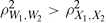 .Footnote 2
Applying this result to the problems of constraint and stability reveals that measurement error in individual survey items will lead to underestimation of the true correlations. Suppose the individual's true preference on issue i at time t is X it. Under a strong version of ideological constraint, where there is a single latent dimension, W i = X + e i for i = 1,2. In this case,  and ρX 1,X 2 = 1, so

Under a strong version of stability, where true preferences and beliefs do not change at all over time, W t = X t + e t for each survey respondent. Consider two periods, t = 1,2. If preferences are perfectly stable over time, then W t = X + e t, and again  .
Critiques of Converse (Reference Converse and Apter1964) by Achen (Reference Achen1975), Erikson (1975), Feldman (Reference Feldman1989), and others followed this line of reasoning. Using the specification of Lord and Novick (Reference Lord and Novick1968) in which the parameters of the measurement error model in a three-wave panel are exactly identified under a set of assumptions, Achen finds that the true correlations in attitudes over time are plausibly as high as .7 or .8, rather than .2 to .45 as Converse found. Under alternative assumptions, Achen (Reference Achen and Finifter1983) arrives at lower estimates of the true correlations for these data. In a five-wave panel, Feldman (Reference Feldman1989) finds correlations closer to those in Achen (Reference Achen1975). These papers deal only with stability over time rather than constraint. With the exception of Feldman these studies are highly dependent on modeling assumptions and do not have the degrees of freedom to test the validity of assumptions. The upshot of this research is that measurement error may produce substantial bias. The challenge is to reduce measurement error without relying on exact identification.
Using Multiple Measures to Reduce Measurement Error
Multiple survey items, combined either as a simple average or as a score using factor analysis, reduce measurement error at the rate of approximately 1/K, where K is the number of items. Here we show the statistical gain from constructing scores in the context of the measurement error model and use these results in the next subsection to show how to estimate the measurement model.
There are two sets of items, each with K elements, {W 11, W 12,. . .,W 1K} and {W 21, W 22,. . .,W 2K}. These might be K repeated questions in a panel at periods 1 and 2, or two distinct sets of questions in the same survey. Suppose each item in the first set taps issue 1 and each item in the second set taps issue 2. That is, W ik = X i + e ik, for each i = 1,2 and k = 1,. . .,K. X i is the true attitude on issue i, and e ik is a random error term with E[e ik] = 0 and  . As above, assume that the measurement error in each item is uncorrelated with the true value of the item itself, uncorrelated with the true values of all other items, and uncorrelated with the measurement error in all other items; i.e., E[X ie jk] = 0 for i = 1,2, j = 1,2, and k = 1,. . .,K, and E[e ike jl] = 0 unless i = j and k = l. Finally, let
 for i = 1,2.
Consider the variables made by averaging the individual items:

Let  and
 be the average measurement error variance among the items in sets 1 and 2, respectively. It is straightforward to show that:




As K becomes large,  and
 become small, and
 increases towards
 . If K = 10, then the contribution of measurement error to the correlation coefficient is roughly one tenth as large as when a single item is used. Also, for each
 decreases toward
 as K becomes large.
Note that we have assumed no autocorrelation in the errors; that is, E[e 1ke 2k] = 0 for all k. Autocorrelation introduces an additional source of bias. However, it is still the case that tends toward as K increases.Footnote 3
Using these results we can immediately address two design considerations that bear on the number of items used to construct the scales.
(1) How closely will the correlations using K items approximate the true correlations? The answer depends on the ratio of signal to noise in the items. Clearly, when there is less measurement error in each item, fewer items are required to achieve the same approximation to the true values. Achen's analysis suggests that the variance in the measurement error in the ANES is approximately equal to the variance of the true issue scales. If that is approximately right, then the true correlation is approximately equal to (K + 1)/K times the observed correlation (between the average measures).
(2) What is the value of adding another item to a scale? For large values of K, one should add another item if the variance of the measurement error in the item is less than twice the average measurement error in the existing set of items. The objective is to minimize mean squared error, that is, to minimize E[![$\overline W_i\,{-}\,X_i]^2 = \overline \sigma_{e_i}^2/K = (\sum_{k=1}^K \sigma_{e_{ik}}^2)/K^2$](https://static.cambridge.org/binary/version/id/urn:cambridge.org:id:binary:20151024010951996-0719:S0003055408080210_inline17.gif?pub-status=live) . Suppose we begin with K items and consider adding item K + 1. Equations (1) and (2) also reveal conditions under which adding additional items improves matters and when it does not. Adding item K + 1 changes the maximand to
 . This is less than
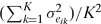 if and only if
 . Note that for large K this reduces to the simple rule of thumb: Add an item if and only if the variance of the measurement error in that item is less than twice the measurement error of the existing items.
Even though the results have the flavor of the sampling theory, the reduction in measurement error does not necessarily occur uniformly. Adding more variables to a scale will tend to make for a better measure, but it is possible to make a scale worse by adding a variable that has an extremely high amount of measurement error. Improvement in the measures depends on the quality of measures as well as their number.
Estimating Parameters of the Measurement Error Model
It is straightforward to estimate the main parameters of interest in the model above. We will focus on the case where 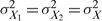 and
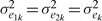 for all k = 1,. . .,K. Although the model can be estimated under more general conditions, this case is sufficient for the purposes of our paper.
Note first that  , and equation (3) can then be written as

Next, note that the intertemporal correlation for each individual item k can be written as

Letting  and averaging over k in (6) yields

So, solving (5) and (7) we have
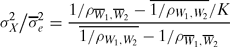

Equation (8) gives a measure of the average signal to noise ratio, and (9) gives the true correlation between issues 1 and 2. These are both easily computed from the underlying correlations of the individual items and the variables made by averaging.Footnote 4
MEASUREMENT ERROR AND PREFERENCE STABILITY
In this section we show that measurement error is a severe problem in individual survey items, but taking multiple items and averaging can dramatically reduces this error. The resulting scales based on multiple measures are highly stable over-time, and scales based on subsets of enough questions are highly correlated within survey. In many cases the over-time correlations are as high as the over-time correlation for the question addressing party identification.
To get a sense of the problem of measurement error, consider, for example, the abortion issue. The National Election Study and other surveys usually measure opinions on this complicated issue with just a single item. A standard form of the question asks:
There has been some discussion about abortion during recent years. Which one of the opinions on this page best agrees with your view on this issue? (1) By law, abortion should never be permitted. (2) The law should permit abortion only in case of rape, incest or when the woman's life is in danger. (3) The law should permit abortion for reasons other than rape, incest, or danger to the woman's life, but only after the need for the abortion has been clearly established. (4) By law, a woman should always be able to obtain an abortion as a matter of personal choice. (5) Other.
A critical reading of this question reveals considerable ambiguity. The categories do not fully cover all possible responses along the given dimension. One can imagine cases between (1) and (2) or between (3) and (4). Some of the categories, especially the third, may encompass a wide range of opinions. Correlation of this item over successive waves of surveys shows that responses to some of the categories (especially 2 and 3) are very unstable while others are not, indicative of measurement problems caused by question wording.Footnote 5 In addition, the categories leave out other very important dimensions to the issue, such as the time during the pregnancy, or the permissibility of in vitro fertilization or embryonic stem cell research. They force respondents into a choice that only partly reflects actual opinion. A stunning example is that 30% of those who chose option 4 also support a ban on partial-birth abortion. A single question seems insufficient to capture the range of preferences on this complicated issue. However, if we add together the several items on abortion (including general abortion attitudes, stem cell research, and partial birth abortion) the resulting score is much more stable over time than the individual items.
Data Sources and Factor Analysis Results
To establish this more generally, we use the 1956–1960, 1972–1976, 1990–1992, and 1992–1996 panel data sets from the National Election Studies. We study the first and last years of each panel, because these typically contain the largest batteries of repeated issue questions. We selected all available questions on public policy issues, plus a few “feeling thermometer” items for particular groups—labor, big business, poor people, welfare recipients, and women's groups—to increase the number of items available for scaling. We grouped these according to issue area.
We consider all issue areas for which we have at least 10 survey items that are repeated in both years of the panel. In addition, because of its key role in Converse's original article and the early debate, we analyze one issue area from the 1956–60 panel—Economic Issues—even though we only have four repeated survey items for it. We also include Law and Order Issues from the 1972–76 panel, even though we have only six repeated items, to increase the variety of issue areas covered in our study. The items used are shown in the Appendix.
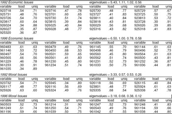
We scaled the items using principal factors factor analysis. In all cases we find a single dominant dimension. The eigenvalues and factor loadings for the 1992 and 1996 economic and moral issues are shown in Table A.1 in the Appendix. (The full set of results takes several pages to present and is available from the authors on request.) We then computed the factor scores for the first factor, and use these scores as our issue scales.Footnote 6
There is nothing magical about the factor scores. In fact, up to an affine transformation they are almost exactly what we get by simply averaging the survey items. For each issue, we oriented each survey item so that higher scores mean more “conservative” positions on the issue, standardized them to have mean 0 and variance 1, and then took the simple unweighted average. The correlation between the simple averages and the factor scores are all .97 or higher, and 13 out of the 18 correlations are .99 or higher. This is not surprising, because the factor loadings are roughly similar across most survey items (see Table A.1). Also, we get essentially identical results if we normalize each item by setting the minimum value to 0 and the maximum value to 1 rather than standardizing.
We use factor analysis in order to separate the first dimension of preferences from any higher dimensions. Throughout we assume a one-dimensional model of preferences. Comparing results using the first factor and the simple average of individual items reveals that the two approaches are nearly identical. This further suggests that, at least in the ANES data, preferences on each issue are mainly one-dimensional.
Intertemporal Stability of Issue Scales
Analysis of issue scales, rather than single survey items, reveals a very high degree of stability in issue preferences. (1) Issue scales are much more highly correlated over time than are individual items. (2) With enough questions, some issue scales are as stable as party identification. (3) Adding more questions the scales become more stable over time, in a manner consistent with the simple measurement error model analyzed above.
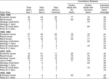
Following Converse, we take simple correlations among scores over time or within surveys to gauge the degree of stability and constraint. For each issue area, we construct the factor scores in the first and last years of the panel. We then compute the correlation coefficient between the scores in the 2 years. These correlations are in columns 4 and 5 of Table 1. In column 5 we construct each issue scale using only the survey items that appear in both years of the panel. In column 4 we construct the issue scales using all available questions in each year—some of these appear in both years and some appear in just 1 year. The results are almost identical in both columns, so neither choice appears clearly superior.
Correlations Between ANES Panel Waves, Issue Scales, and Individual Survey Items

Note: The number of observations (N) varies slightly from cell to cell due to missing data. For the Economic Issues scales made using all common items, N = 534 in the 1992–96 panel; N = 607 in 1990–92; N = 971 in 1972–76; and N = 953 in 1956–60.
The intertemporal correlations of the issue scales are quite high: the average correlation is .77 for the five issue areas of 1990–92 and 1992–96. This is much higher than the average correlation among individual survey items, which is just .46. No issue scale has a stability coefficient below .63.
General questions on ideology also exhibit more stability when scaled, even with just three items.Footnote 7 Single-item ideology measures have intertemporal correlations of approximately .55, whereas scales constructed from those items have intertemporal correlations in the neighborhood of .7 to .75. Providing further evidence of measurement error, the 7-point ideology questions are more stable than the 3-point ideology questions.
Perhaps most striking, the issues scales exhibit a degree of intertemporal stability on par with party identification. The average intertemporal correlation is .77 among the issue scales and .79 among party identification. None of the issue scales in 1972–72, 1990–92, or 1992–96 panels are markedly less stable than partisanship. This is an important result, because the relatively high level of stability found for party identification is often taken as evidence that party identification is something real, solid, and meaningful in public opinion.
Party identification may be measured with error as well, and the intertemporal stability of “true” party identification is probably even higher than .8 (Green and Palmquist, Reference Green and Palmquist1994; Green, Palmquist, and Schickler Reference Green, Palmquist and Schickler2002). A three-item partisanship scale, however, does no better than the single-item scale. This suggests that the extra two items—feeling thermometers for Democrats and Republicans—have considerably more measurement error than the 7-point party identification scale.
Comparing the different studies, we see that the earlier panels produced scales with lower intertemporal correlations than later panels. This might reflect the rise of issue voting in the mid-1970s. We suspect it arises from the small number of items in the earlier panels.
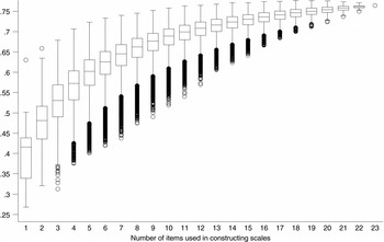
Figure 1 shows the intertemporal stability of a scale as a function of the number of items in a scale. The analysis is of the 1990 and 1992 Economic Issues scales. We performed a Monte Carlo simulation in which we randomly chose an appropriate number of items (from 1 up to all 23), constructed the scales, and computed the intertemporal correlations of the scales.Footnote 8 The plot displays the median intertemporal correlations plotted against K, together with the interquartile range, in a box-and-whiskers plot.
Correlation Between 1990 and 1992 Economic Issue Scales Box-and-Whiskers Plot

The intertemporal stability of the issue scales rises smoothly and concavely with the number of survey items used. In this particular case (Economic Issues in 1990–92), the typical single item exhibits stability of .41, far below the actual correlation. That gap shrinks as the number of items increases, and at 23 items, the intertemporal correlation averages .76, close to its upper limit of .79.
The pattern in Figure 1 allows us to put the 1952–56 panel in context. That panel had only 4 items in common across all waves and a stability coefficient on the 4-item scale of .63. However, using 4 randomly chosen items in the 1990–92 economic issues to construct a scale produced a typical correlation of .57. The 1952–56 panel, then, shows as much stability as the later panels, but that study simply included too few questions to reduce the measurement error fully. The 1972–76 panel had 11 items concerning economic issues; the level of stability in that study is consistent with the graph as well and suggests that a larger number of items would produce even more stable measures of issue preferences.
Equation (8) allows us to use the figures in the graph to calculate the amount of measurement error in the typical survey item. Recall that equation (8) gives an estimate of the average signal to noise ratio in the individual survey items, and the intertemporal stability of the underlying preferences.Footnote 9 Applying this to the items in the 1990 and 1992 Economic Issues, the average signal to noise ratio is about .95. This implies that on average about half of the variance in individual survey items is from actual issue positions and half is from measurement error. This is approximately what Achen (Reference Achen1975) found for the 1958 to 1960 panel using a very different methodology.Footnote 10
The high degree of intertemporal stability of the scales, displayed in Figure 1, need not have emerged. Little relationship between the number of items and the correlations of the scales would have emerged if either (1) responses to the questions were primarily noise or had little stability, or (2) there were many dimensions underlying the data. A high degree of heterogeneity among the respondents, as with Converse's Black-White model discussed below, would also have prevented the correlations from approaching the true correlations in the asymptotes, because a large fraction of people would have 0 correlations in their answers. Rather correlations increase monotonically in the number of items in the scale; this holds true for the entire sample and for high and low sophistication people.
Within-Survey Stability of Issue Scales
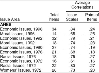
We can also examine the within-survey, cross-sectional stability of issue scales. This is what Converse (Reference Converse and Apter1964) and others call “constraint.” Consider a given issue area in a given year, and suppose the total number of associated survey items is M, with M even. We can divide these items into two disjoint subsets, each with M/2 items, then scale each subset separately and calculate the correlation between these scales. We calculate the average correlation, because there are many possible partitions of the M items.Footnote 11
The results of this analysis are shown in Table 2, which includes all issue areas and years for which we have 14 or more total survey items (so that each scale is made with at least 7 items). As expected given the pattern of eigenvalues shown in Table A.1, the correlations between the scales are quite high—in most cases higher than .70. Moreover, they are much larger than the average correlations among the individual items that went into the construction of the scales, which range from .16 to .27.
Correlations Between Issue Scales of Disjoint Subsets of Half of the Items

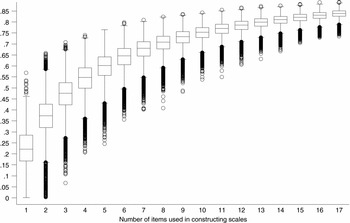
Figure 2 shows how the correlations depend on the number of items scaled, analogous to Figure 1. The figure examines the 1996 ANES economic issues. There are M = 34 relevant items in the survey, which allows us to study the stability of scales made from up to 17 items, K = 1,. . .,17. For each value of K, we implement the following procedure. Draw two disjoint subsets, each of size K, from the 34 questions, scale each subset separately, and calculate the correlation between the resulting scales. We calculate the average correlation, since there are many possible disjoint subsets for each value of K. As in the construction of Figure 1 and Table 2, we use Monte Carlo techniques to construct our estimates.
Correlation Between Various 1996 Economic Issue Scales Box-and-Whiskers Plot

Figure 2 shows the resulting median correlations plotted against K, together with the inter-quartile range, in a box-and-whiskers plot. As in Figure 1, the average degree of stability (constraint) rises smoothly and concavely as the number of survey items increases. With 17 questions the average correlation is .84, fairly close to its theoretical upper limit of 1.00.
The analysis reflected in Figures 1 and 2 suggests the enormous amount of measurement error in single survey items used to capture issue preferences. The analysis points to a specific solution as well. Survey researchers should use multiple items—and the more the better.
Policy Positions versus Policy-Related Predispositions
As noted in the introduction, numerous scholars have argued that while voters may not have stable preferences over particular policies or issues, they do possess “core values” or “predispositions” that are coherent and stable (McClosky and Zaller Reference McClosky and Zaller1984; Feldman Reference Feldman1988; Zaller Reference Zaller1992). Since the 1970s the ANES has included several subsets of items designed to tap into these predispositions. We included these items in the batteries used to construct the issue scales analyzed above. It is therefore possible that most of the stability we find is due to the inclusion of these items.
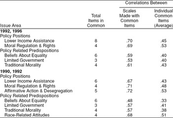
To examine this possibility, following Miller and Shanks (Reference Miller and Shanks1996), we constructed “policy related predisposition” scales for the 1990–92 and 1992–96 panels. These are Beliefs About Equality, Limited Government, Traditional Morality, and Race-Related Attitudes. We also constructed several “policy position” scales based solely on questions that refer to specific policies or government activities. We call these Lower Income Assistance; Moral Regulation & Rights; and Affirmative Action & Desegregation. The Appendix gives the exact survey items used for each scale.
Table 3 shows the results. Once again, in each row the issue scales show substantially more stability than the average for the individual items. More importantly, when we focus on particular issues using purely policy questions, the resulting scales are even more stable over time than the “predisposition” scales. For instance, for the 1990–92 panel, the intertemporal correlation for a scale constructed from six questions about assistance for low-income individuals was .67, whereas that for six questions tapping beliefs about equality was .48. The correlation for a scale based on policies related to moral regulations and rights was .71, while that for predispositions related to traditional morality was .57. The story is similar for the 1992–96 panel. Only in the area of race and affirmative action do policy positions and predispositions show roughly similar levels of stability.
Correlations Between ANES Panel Waves, Policy Positions vs. Policy-Related Predispositions

Heterogeneity in Political Sophistication
The standard measurement error model laid out above treats all individuals similarly. Survey researchers, however, have long argued that citizens vary widely in their degree of “political sophistication” (e.g., Luskin Reference Luskin1987; Saris and Sniderman Reference Saris and Sniderman2004). For example, Converse (Reference Converse and Apter1964) rationalizes the low overall correlations in survey responses as reflecting a heterogeneous population, of which a small fraction understand complicated public policy matters, have well formed preferences, and answer survey questions without error. The remaining majority—the unsophisticated—appear to answer questions almost at random. Converse terms this the Black-White model.
Here we examine this issue in the context of issue scales. Although we do find evidence of heterogeneity, consistent with Feldman (Reference Feldman1989), measurement error is the larger issue.
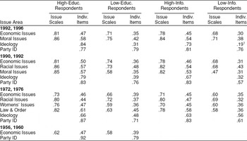
A first step is to examine how measurement error varies across levels of political sophistication. Table 4 reports intertemporal stability correlations analogous to those in Table 1, broken down by high versus low education levels (following Converse Reference Converse and Apter1964), and high versus low levels of political information (using the interviewer assessments favored by Zaller (Reference Zaller1992) and others). The high-education group consists of individuals with college degrees or more. The low-education group consists of those with a high-school degree or less. Interviewers were asked to rate each respondent's “general level of information about politics and public affairs” on a 5-point scale ranging from 1 = “very high” to 5 = “very low.” The high-information group consists of individuals rated “very high” or “fairly high,” whereas the low-information group consists of those rated “very low” or “fairly low.”
Correlations Between ANES Panel Waves, Issue Scales, and Individual Survey Items by Education and Political Information Level

Note: In each case, the issue scales are made using only the survey items common to both years of the panel. The number of items for each issue area can be found in Table 1, column 3.
There is clear evidence of some heterogeneity. The intertemporal correlations for low-education and low-information individuals are uniformly lower than the corresponding correlations for high-education or high-information individuals. This is true for the issue scales, and also for the individual survey items underlying the scales. It is also true for self-placed ideology, and for party identification (except in one case).
It is equally clear, however, that the responses of both high-information and low-information individuals are plagued with a large amount of measurement error. In the 1992–96 panel, the intertemporal stability of the Economic Issues Scale for high-education individuals is .81, whereas for low-education respondents it is .71. But the average intertemporal stability of the individual items that comprise the scale is .47 for high-education individuals and only .35 for low-education individuals. Using equation (8), we estimate a signal to noise ratio of 1.22 for high-education individuals and 0.81 for low-education individuals. These are intuitive, implying a bit more signal than noise in the responses of the high-education group, and a bit more noise than signal in the responses of the low-education group. Also, although different, they are in the same ball park.
Note also that for both high-education and low-education individuals, the intertemporal stability of the Economic Issues Scale is much higher than the stability of self-placed ideology, and nearly as high as the stability of party identification. These general patterns hold for other scales and other years as well.
One can criticize the analysis above on the grounds that measurement error also plagues our measures of political sophistication. We may understate the importance of heterogeneity if we have misclassified many high-information respondents as having low-information, and vice-versa. In fact, we can construct better measures of political sophistication by combining multiple items. We constructed one such measure for the 1992–96 panel using education, the interviewer assessment, and the answers to any factual questions asked in the panel, such as which party controls the U.S. House, which party controls the Senate, who is William Rehnquist, and who is Boris Yeltsin. Interestingly, the resulting scale is much more stable over time than any of the individual items. Even the interviewer assessment is fairly unstable—the intertemporal correlation is just .55. By contrast, the intertemporal correlation of the scale is .77. Replicating the analysis discussed above using the scaled measure of political sophistication leads to qualitatively similar results to those reported in Table 4. For example, dividing the sample at the mean value of the sophistication scale, the intertemporal stability of the Economic Issues Scale for “high-sophistication” individuals is .81, while for “low-sophistication” respondents it is .66.
Finally, we can refine the analysis further by switching the focus from correlations to variances. When we do this the bottom line is the same. On one hand there is evidence of heterogeneity with respect to levels of sophistication. We cannot tell if this is due to differences in measurement error or differences in the distribution of underlying preferences, but there are clearly differences of some sort. Consider, for example, Economic Issues Scale for 1992.Footnote 12 The variance of the average of the 23 survey items,  , is .21 in the entire sample. Examining subsets, we see that is almost monotonic in the level of sophistication, declining from .39 for the group with a “very high” level of political information to .18 for the group with a “very low” level of information.
Perhaps more importantly, the variances provide further evidence that even the least sophisticated are not merely “guessing” when answering issue questions. If these respondents were simply guessing, so their responses were purely random noise, the variance of the average of 23 items would be 1/23 = .043. As noted, the variance among the group with “very low” political information is .18, more than four times larger than the predicted value under a null hypothesis of pure noise. Thus, the answers of even this least sophisticated group of respondents have much more content than Converse asserted.
ISSUE VOTING
Perhaps the most damning empirical result for issue voting is the fact that individual issue items rarely show large, statistically significant, and robust effects in explaining voting preference or approval of elected officials. By contrast, party identification is always found to be extremely important in predicting vote choice and approval. Kinder (Reference Kinder1998) surveys the vast number of studies on this subject and aptly characterizes issue voting as of marginal importance in the literature.
In this section we argue that measurement error is a major reason for this conclusion. If individual survey items contain a large amount of measurement error, then it is likely that most of the literature on issue voting has underestimated the effects of issues on electoral decisions. It is well known in statistics that measurement error in independent variables biases estimates of regression coefficients. Measurement error has two effects. First, measurement error creates bias and inconsistency in the independent variable that is measured with error. Typically, the effect of measurement error is to shrink the estimated effect toward zero. If only one variable is measured with error, then the coefficient on that variable will be biased toward zero. When many variables contain measurement error, biases may take more general forms, including incorrect signs (e.g., Klepper and Leamer Reference Klepper and Leamer1984). Second, measurement error on one variable spills over onto other variables. Because all coefficient estimates depend on the variances and covariances of all variables, measurement error in one variable necessarily affects the estimated coefficients on other variables.
Similar to Erikson and Tedin (Reference Erikson and Tedin2007), we show that correcting for measurement error by averaging together multiple measures produces a radically different conclusion about the relative importance of issue positions on vote choice. Issues have statistically significant and substantively large effects, comparable in magnitude to the effects of party identification.
To do this, we contrast two sorts of estimates. First, we regress voting decisions on party identification, ideology, and a battery of individual issue items. Second, we construct issue scales from the individual issue items, and use these as independent variables in place of the items. If issues matter for voting but measurement error in the individual issue items is a substantial problem, then the estimated coefficients on these variables will tend to be attenuated and few will be statistically significant. The coefficients on the scales will be much larger than the coefficients on the individual items, and the scales will be highly significant.
We have followed this approach with a number of surveys and obtained similar results, but due to space constraints, we present the results from the American National Election Studies of 1992 and 1996. For each of these surveys, we identified two to three dozen issue questions likely to matter directly to the vote. We constructed two scales—an Economic Issues Scale using all items on economic issues, and a Moral Issues Scale using all items on moral and social issues.Footnote 13
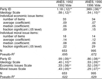
Table 5 contrasts the evidence of issue voting using individual issue items and the scaled issue measures. The top panel displays the results of probit regression analyses predicting the Republican versus the Democratic vote for president as a function of party identification, an ideology scale, and issue positions on all the relevant questions. In order to aid comparisons, we standardized all of the regressors. The vote is coded as 1 for Republican and 0 for Democrat (we drop respondents who voted for minor candidates or did not vote). Rather than show a large number of small and insignificant coefficients, we display the average and median of the absolute values of the coefficients, and the fraction that are statistically significant at the .05 level. The bottom panel shows the results using the three issue scales in place of the individual issue items.
Effects of Party and Issues on Presidential Voting

Note: All variables standardized.
** = significant at the .01 level.
** = significant at the .05 level.
The results are broadly consistent with the conjecture that there is substantial measurement error bias in regressions that use individual items to capture voters' issue positions. When we use individual issue items, the coefficients are small and few are statistically significant. Consider, for example, the 1992 ANES. When we use the individual issue items, only one in ten economic issue coefficients, and one in five moral issue coefficients are statistically significant at the .05 level. The average absolute values of the coefficients are .09 and .14. In 1996 the average absolute values of the coefficients are slightly lower, although a slightly larger fraction are statistically significant.
When we combine the individual items to construct issue scales, however, the picture changes dramatically. Issue preferences suddenly appear to have much larger and more robust effects on the vote. In both analyses, the coefficients on the “economic issues” and “moral issues” scales are large and statistically significant at the .01 level. In the 1996 ANES, the coefficient on the Economic Issue Scale is more than twice as large as the largest coefficient on any of the individual economic issue items. In both regressions, the combined effect of changing both the Economic Issues Scale and the Moral Issues Scale by 1 standard deviation (SD) is nearly as large, or even larger than, a change of 1 SD in party identification. The coefficient on the Moral Issues Scale is the same size as the coefficient on the Economic Issues Scale in the 1992 ANES, but smaller in the 1996 ANES.Footnote 14 Moral issues are significant in all three analyses, and the scale always has a larger coefficient than any of the individual moral issue items.Footnote 15
Heterogeneity, along the lines of Converse's Black-White model, would manifest itself as interactions in these specifications. Specifically, high information and interest individuals would have definite issue preferences, and their expressed opinions would translate directly into votes. However, low information and interest individuals are thought to have no well defined attitudes. According to the Black-White model, low-information voters' responses to issue questions are largely noise and, thus, bear no relation to their vote choice. This model is surely an extreme case, but substantial heterogeneity may still operate if those with higher levels of information are noticeably more issue-oriented in their voting.
What, then, is the relationship between level of information or education and issue voting? The answer, evidently, is none. We reanalyzed the specifications in Table 5 including measures of information and interactions between the issue scales and respondents' information or education.Footnote 16 Education has a significant main effect on the vote, reflecting the fact that higher educated Americans tend to be more Republican. None of the interactions are statistically significant, and the magnitudes of the estimated interactions are small and substantively unimportant. In the 1996 ANES, the estimated interaction between high education (college or more) and the Economic Issues Scale is −.08 with a standard error (SE) of .18, and the estimated interaction between high education and the Moral Issues Scale is −.07 (SE = .19). By contrast the main effects are .55 for the Economic Issues Scale and .44 for the Moral Issues Scale. When we used the interviewer's rating of respondents' information levels to measure sophistication, the interactions are .16 (SE = .17) and −.18 (SE = .17) for economic issues and moral issues, respectively. In neither survey does the likelihood ratio test reject the hypothesis that all of the interactions equal 0. There is, then, little evidence that sophistication magnifies the extent to which issue preferences affect the vote.
This is a striking conclusion in light of the large literature that looks for such interactions (e.g., Delli Carpini and Keeter Reference Delli and Keeter1996; Goren Reference Goren1997). The fact that the issue scales do not interact with sophistication in predicting the vote carries the implication that such interactions in studies using single items to measure issue preferences are likely capturing measurement error, not substance. Survey respondents with high education and high information may simply be better test takers, not better citizens.
CONCLUSIONS
The implications of our analysis are at once methodological and substantive. At least since Achen Reference Achen1975, political scientists have recognized the potentially serious biases introduced by measurement error in single survey items. We have documented that those errors are indeed large, and the consequences for our discipline are far-reaching, owing to the centrality of survey research to political science.Footnote 17 We have focused on just one important line of inquiry, and discovered that measurement error has led the field to under estimate the extent to which the electorate holds and relies on their policy preferences.
Three basic methodological lessons emerge. First, measurement error is substantial, even in high-quality surveys such as the ANES and GSS, where approximately half of the variance in responses across individuals within the typical issue item is attributable to measurement error, and the other half reflects true differences in preferences. This finding suggests caution in drawing inferences from analyses of surveys that focus on single items introduced to capture issue preferences.
Second, averaging offers a simple and time-honored way to reduce the measurement error long known to corrupt individual survey items and the resulting bias in regression models. Others have used factor analysis to uncover latent dimensions of preferences, but political scientists have not appreciated the degree to which factor analysis and other methods of averaging can fix measurement error of the sort that arises from vague questions and categories that attempt to capture the complexity of public opinion on a topic with a single question, or from distraction or boredom of the respondent. Multiple measures should, of course, be used with care. Among other things, it is important to examine the consistency and reliability of one's scale and to justify the inclusion of items (see, e.g., McIver and Carmines Reference McIver and Carmines1981). Moreover, it may be necessary to address the problem of nonrandom measurement error (see, e.g., Green and Citrin Reference Green and Citrin1994). How best to use multiple measures is an important avenue for further development.
Third, we encourage those engaged in the design of surveys to focus on the quality of batteries of questions, not just individual items. There are two ways to reduce measurement error: ask better questions and ask more questions. These two are not at odds. Although the ANES and GSS pilot and vet their questions carefully, substantial measurement error remains. Further efforts to improve the quality of questions are valuable, but often, no single survey question can capture the complexity of opinion on a given issue or issue cluster. The work here on Economic and Moral issues is a start, but a more in-depth consideration of these and other aspects of issue voting (notably race, civil liberties, and foreign affairs) is in order. We recommend a systematic effort to develop batteries of questions designed to capture issue preferences rather than focusing on single items.
The lessons here also extend to other survey research problems, especially measuring ideology and citizen knowledge. Congressional studies have long used roll call vote scores to measure ideology, but survey researchers have used a single item in which respondents use terms such as “liberal” and “conservative” to describe their ideology. The approach of congressional scholarship to the measure of ideology seems particularly promising, as the terms liberal and conservative may not fit people's belief systems well. Measurement of knowledge has seen the most use of multiple measures in the survey world, but there is still considerable disagreement about what is an appropriate measure. Zaller (Reference Zaller1992) discusses the advantages of using multiple measures to capture knowledge, but in the end, settles on a single best indicator based on the interviewer's evaluation. However, a preliminary analysis of the measures Zaller examined suggests that averaging together multiple measures of knowledge produces a measure with higher construct validity than any single item. These themes await more concerted examination in their own right.
Sometimes the value of improved methods lies in convincing us more firmly of an accepted wisdom. Other times the value is in allowing us to see things that were previously obscured from view. The empirical analysis in this paper comes closer to the latter than the former. Although others have come before us, our rather simple approach to measurement error yields a markedly different picture of belief systems in mass publics and issue voting than the consensus view that still holds sway over the textbook descriptions of the American public.
First and foremost, we find strong evidence that voters have stable policy preferences. Converse (Reference Converse and Apter1964) famously concluded that the mass of the electorate holds nonattitudes on important policy questions, such as race relations, foreign affairs, and economic redistribution. His evidence was twofold. The correlation among individual items on each of these questions was relatively small, suggesting little “constraint,” and individual's responses to a given item were unstable over time. The correlations he found ranged from .2 to .4. Upon averaging items we find much more evidence of constraint and stability. The correlations among the averages of half-samples of items approaches .8, as do the over-time correlations of the individuals' issue policy scales. If the vast majority of people have nonattitudes, as Converse conjectured, averaging would have again returned low correlations.
Second, issues matter to the electorate. The vast majority of research on the topic finds weak or no evidence that issue preferences explain the vote. But, those studies rely almost entirely on single items to measure voters' policy preferences. A small minority construct scales, analogous to roll-call voting scores, and that branch of the literature finds substantively important effects of issues (e.g., Carmines and Stimson 1980; Erikson and Tedin Reference Erikson and Tedin2007). Ansolabehere, Rodden, and Snyder (Reference Ansolabehere, Rodden and Snyder2006) show that issue scales like those used here for presidential elections are also very good predictors of vote choice in U.S. Congressional elections, and Heath et al. (Reference Heath, Evans and Martin1994) construct issue scales that are powerful predictors of vote choice in British parliamentary elections. Issue scales constructed from questions in the World Values Survey have also been used to understand vote choice and other forms of political behavior in cross-national studies such as Inglehart (Reference Inglehart1990) and more recently, De La O and Rodden (Reference De and Rodden2008).
We argue that the tension in the empirical literature stems from measurement error in individual issue items. When we use individual items to measure policy preferences, we find relatively little evidence of issue voting. However, consistent with a simple model of measurement error, we find strong evidence of issue voting when vote preference is regressed on issue scales, controlling for party identification and ideology. In fact, contrary to the bulk of the literature, we find that issue voting may rival party in explaining the vote. The combined effects of issue preferences are about as large as party identification in the multivariate analyses predicting the vote.
Third (and certainly worthy of deeper investigation), heterogeneity of sophistication among the public is not as important a phenomenon as the line of inquiry from Converse through Zaller would suggest. Converse distinguished two sorts of citizens—a relatively small group with high levels of education and political sophistication, and a great mass of unsophisticated voters whose responses to policy-related survey questions are essentially guesses. Yet we find that the over-time correlations of policy preference scales among low sophistication respondents are typically in the range of .6 to .7. These are much larger even than the levels Converse observed for single items among high sophisticates, and not much different than the intertemporal stability found by Jennings (Reference Kent1992) on three issue items in a study of a group of highly sophisticated elites—delegates to national party conventions.
The least educated or sophisticated voters do appear to have somewhat less stable policy opinions than those with high education or sophistication. But, the difference between these two groups is small compared with the enormous amount of measurement error in individual survey items on policy issues. Correcting for the measurement error, all groups exhibit considerable policy content to their opinions.
Moreover, what heterogeneity we do observe has little direct effect on vote choice. Models such as Converse (Reference Converse and Apter1964) and Zaller (Reference Zaller1992) imply that we should observe strong interactions between sophistication and policy preferences in predicting the vote. We find no such interactions. Neither education nor political information magnifies the extent of issue voting. All respondents draw equally strongly on their policy preferences in choosing elected officials.
Our findings are encouraging for theoretical models of elections and representation that rely on spatial representations of preferences. Converse's nonattitudes finding has been something of a show stopper for the spatial theory of elections. If voters do not have policy preferences, how could such models possibly characterize elections? Erikson, MacKuen, and Stimson (Reference Erikson, MacKuen and Stimson2002) suggest that a meaningful policy “signal” is produced by averaging many millions of votes. Our findings imply an even simpler story: there is substantial policy content to individual voters' preferences and behaviors, but the survey instrument has not been sufficiently finely tuned to detect it. Using multiple measures to capture issue preferences offers a way to solve long-standing puzzles concerning the nature of belief systems in mass publics.
APPENDIX
Here we list the variable numbers of the survey items used in constructing each of scales in the paper. The items in parentheses appear in only one survey of the panel. These are used for the scales made with all items but not for the scales made with common items.
Factor Analysis Results
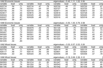
Note: Here we present summary statistics from the factor analyses used in constructing some of the scales using common items.
1992 Economic Issues: 923701, 923716, 923718, 923725, 923726, 923727, 923728, 923730, 923811, 923813, 923815, 923817, 923818, 925316, 925318, 925320, 925729, 925730, 925731, 926024, 926025, 926026, 926027, 926028, 926029, (923717, 923729, 923745, 923746, 923816, 923819, 926137)
1996 Economic Issues: 960450, 960479, 960483, 960496, 960497, 960498, 960500, 960501, 960560, 960561, 960562, 960564, 960565, 961033, 961035, 961036, 961229, 961230, 961231, 961232, 961233, 961234, 961144, 961145, 961146, (960537, 961219, 961220, 961226, 961227, 961283, 961320, 961322, 961324)
1992 Moral Issues: 923732, 923801, 925324, 925335, 925338, 925924, 925926, 925945, 926115, 926116, 926117, 926118, (923736, 923738, 923740, 925928, 926020, 926119)
1996 Moral Issues: 960503, 960543, 961038, 961039, 961042, 961194, 961196, 961214, 961247, 961248, 961249, 961250, (961043, 961199)
1992 Multi-Item Party ID: 923634, 923317, 923318
1996 Multi-Item Party ID: 960420, 960292, 960293
1992 Multi-Item Ideology: 923509, 923511, 923512, 925326, 925319
1996 Multi-Item Ideology: 960365, 960366, 961032, 961031
(Note, 7-point ideology scale item was constructed from underlying branching questions)
1990 Economic Issues: 900157, 900159, 900162, 900331, 900333, 900335, 900377, 900379, 900380, 900382, 900383, 900384, 900385, 900386, 900426, 900427, 900428, 900429, 900430, 900431, 900446, 900488, 900452, (900332, 900487, 900490)
1992 Economic Issues: 925316, 925318, 925320, 925729, 925730, 925731, 926024, 926025, 926026, 926027, 926028, 926029, 923701, 923716, 923717, 923718, 923725, 923727, 923729, 923730, 923745, 923811, 923813, 923815, 923818, (923726, 923728, 923746, 923816, 923817, 923819, 926133, 926137)
1990 Racial Issues: 900386, 900447, 900464, 900466, 900470, 900518, 900519, 900520, 900521, 900522, 900523
1992 Racial Issues: 923724, 923729, 925929, 925930, 925932, 925936, 925948, 926126, 926127, 926128, 926129, (925938)
1990 Moral Issues: 900158, 900330, 900467, 900479, 900481, 900483, 900500, 900501, 900502, 900503, (900154, 900163, 900471, 900472
1992 Moral Issues: 923732, 923736, 923738, 925324, 925945, 926115, 926116, 926117, 926118, 926020, (923740, 923801, 925335, 925338, 925924, 925926, 925928, 926119)
1990 Multi-Item Party ID: 900320, 900151
1992 Multi-Item Party ID: 923634, 923317, 923318
1990 Multi-Item Ideology: 900406, 900407, 900161, 900156
1992 Multi-Item Ideology: 923509, 923511, 923512, 925326, 925319
(Note, 7-point ideology item was constructed from underlying branching questions)
1972 Economic Issues: 720208, 720629, 720707, 720708, 720722, 720737, 720738, 720744, 720753, 721067, 721068, (720214, 720843, 720848, 720856, 720688, 720690, 720693, 721111, 721112)
(Note, 720670, 720686, 720687, 720691, 720692, 720694, 720689 were not used because they were only given to a subsample of respondent's.)
1976 Economic Issues: 763241, 763264, 763273, 763566, 763567, 763573, 763582, 763751, 763752, 763753, 763754, 763755, 763757, 763758, 763767, 763779, 763821, 763822, 763836, (763353, 763589, 763562)
1972 Racial Issues: 720106, 720112, 720115, 720118, 720202, 720727, 720729, 720745, 720845, 720847, 720849, 720855, 720859, 720862, (720104, 720110, 720113, 720114, 720119, 720851, 720857)
1976 Racial Issues: 763211, 763213, 763214, 763217, 763257, 763570, 763803, 763805, 763806, 763807, 763812, 763814, 763841, 763843, (763588)
1972 Womens' Issues: 720232, 720238, 720239, 720725, 720844, 720846, 720850, 720852, 720858, 720860, (720240, 720242, 720243, 720244, 720245, 720246, 720247, 720248, 720249, 720251)
1976 Womens' Issues: 763787, 763796, 763798, 763802, 763804, 763808, 763809, 763811, 763813, 763839, (763574, 763799)
1972 Law & Order & Military: 720196, 720621, 720713, 720714, 720717, 720726, (720678, 720728, 720733)
1976 Law & Order & Military: 763248, 763772, 763827, 763828, 763831, 763840, (763561, 763563, 763565, 763909, 763913)
1972 Multi-Item Party ID: 720140, 720719, 720721
1976 Multi-Item Party ID: 763174, 763833, 763835
1972 Multi-Item Ideology: 720652, 720709, 720724
1976 Multi-Item Ideology: 763286, 763823, 763838
1956 Economic Issues: 560032, 560038, 560053, 560059, (560029, 560047)
1960 Economic Issues: 600618, 600620, 600624, 600632
1992 Beliefs About Equality: 926024, 926025, 926026, 926027, 926028, 926029
1996 Beliefs About Equality: 961229, 961230, 961231, 961232, 961233, 961234
1992 Limited Government: 925729, 925730, 925731
1996 Limited Government: 961144, 961145, 961146
1992 Traditional Morality: 926115, 926116, 926117, 926118
1996 Traditional Morality: 961247, 961248, 961249, 961250
1992 Lower Income Assistance: 923716, 923718, 923725, 923726, 923730, 923813, 923817, 923818
1996 Lower Income Assistance: 960479, 960483, 960496, 960497, 960501, 960562, 960564, 960565
1992 Moral Regulation & Rights: 923732, 925924, 925926, 925945
1996 Moral Regulation & Rights: 960503, 961194, 961196, 961214
1990 Beliefs About Equality: 900426, 900427, 900428, 900429, 900430, 900431
1992 Beliefs About Equality: 926024, 926025, 926026, 926027, 926028, 926029
1990 Limited Government: 900331, 900333, 900335
1992 Limited Government: 925729, 925730, 925731
1990 Traditional Morality: 900500, 900501, 900502, 900503
1992 Traditional Morality: 926115, 926116, 926117, 926118
1990 Race-Related Attitudes: 900520, 900521, 900522, 900523
1992 Race-Related Attitudes: 926126, 926127, 926128, 926129
1990 Lower Income Assistance: 900382, 900383, 900384, 900385, 900446, 900488
1992 Lower Income Assistance: 923718, 923725, 923730, 923745, 923813, 923818
1990 Moral Regulation & Rights: 900467, 900479, 900481, 900483
1992 Moral Regulation & Rights: 923732, 923736, 923738, 925945
1990 Affirmative Action & Desegregation: 900386, 900447, 900464, 900466, 900470
1992 Affirmative Action & Desegregation: 923724, 925929, 925932, 925936, 925948
 . Then Cov(
 . Note that ρ
 (i.e., the “average” autocorrelation in the errors exceeds the correlation in the underlying dimension). If this condition holds, then ρ
 then ρ
 may vary across i. Consider this more general case. The variances for the individual items are
 for i = 1,2 and k = 1,. . .,K. Let
 for i = 1,2. Averaging over k then yields
 for i = 1,2. Combining these with equations (
 and
 for i = 1,2. These equations provide us with average signal to noise ratios,
 and
 . Also, substituting them into (3) and rearranging yields an estimate of the true correlation between issues 1 and 2:
 . Note finally that the model is evidently overidentified and therefore may be tested.
 distinct subsets of K survey items taken from the 23 available items. For each subset S of K survey items, we can construct a scale for 1990 and a scale for 1992, then calculate the correlation

 is a large number (8,388,584), we used Monte Carlo techniques that iteratively drew 500,000 subsets of questions, each time drawing a subset S of survey items and constructing
 distinct subsets of M/2 items. Averaging over all of these subsets produces a measure of the average cross-sectional stability of scales made with M/2 items. Again, since
 ) for each respondent rather than factor scores. Also, in order to obtain as large a sample as possible, we study the entire sample from 1992, including both the panel and non-panel respondents, which gives us 1,217 observations. Recall that each survey item is standardized to have a mean of 0 and a variance of 1.




Comments
No Comments have been published for this article.