1. Introduction
Humanity has made and continues to make significant progress in averting and delaying death which, although indicative of tremendous societal progress, does present economic and social risks to healthcare, social security, private pension systems, and life insurers. The main risk, however, is not increasing longevity per se, but rather the challenges tied to the inherent uncertainty of the future evolution of mortality rates. Dynamic mortality modelling is therefore of critical importance, both to facilitate an understanding of historical mortality patterns and to provide a basis for future mortality projections.
Traditionally, amongst an actuarial readership, generalised age-period-cohort (GAPC) models have been a preferred approach (Villegas et al. Reference Villegas, Kaishev and Millossovich2018; Hunt and Blake Reference Hunt and Blake2021b). These models decompose the force of mortality for age x at time t,
 $\mu_{x,t}$
, across the dimensions of age, x, period (or time), t, and cohort (or year of birth),
 $t-x$
, via the following general specification:
 \begin{equation}\ln(\mu_{x,t}) = \alpha_{x} + \sum_{i=1}^{N} \beta_x^{(i)}\kappa_t^{(i)} + \gamma_{t-x}.\end{equation}
GAPC models, which can be expressed as generalised (non-) linear models (Currie Reference Currie2016), have proven particularly popular due to the ability to simulate future outcomes and develop probabilistic forecast intervals, as well as the direct interpretability of parameters in terms of their demographic significance. For example, the general age shape component of mortality is captured by
 $\alpha_{x}$
, systematic longevity improvements across specific ages over time are reflected by
 $\beta_x^{(i)}$
and
 $\kappa_{t}^{(i)}$
,
 $i=1,\dots,N$
, and any effects embedded in an individual’s year of birth are allowed for by
 $\gamma_{t-x}$
. However, a major drawback to this family of models is the inherent subjectivity associated with the construction and selection of the most appropriate model within the family.
In theory, there are an infinite number of models that can be produced within the framework defined by Equation (1.1), corresponding to every possible combination of terms:
 $\alpha_x$
, N,
 $\beta_x^{(i)}$
, and
 $\gamma_{t-x}$
; where
 $\beta_x^{(i)}$
can be either non-parametric or parametric with various functional forms. In an ideal world, we would be able to consider every possible combination of terms to choose the optimal model for a given data set and application. However, this is clearly not feasible due to time and computational constraints, and as a result, practitioners have been forced to rely on a small, but growing, selection of models, which are outlined in the Section 3.
Citing these issues, Hunt and Blake (Reference Hunt and Blake2014) propose an alternative “general procedure” to construct bespoke mortality models, which involves using “expert actuarial judgement” to manually select appropriate age-modulating terms to capture historical mortality patterns identified within specific data sets. However, whilst data-driven and potentially powerful, the procedure lacks a formalised quantitative framework for implementation, thereby introducing room for subjectivity and inconsistency. Moreover, the overreliance on the historical goodness of fit to select the model specification does not necessarily translate into improved out-of-sample projection accuracy.
The main objective of this paper is to propose an alternative mortality model construction procedure – using regularisation and cross-validation techniques – that mirrors the data-driven framework proposed by Hunt and Blake (Reference Hunt and Blake2014), albeit through a different lens. Whilst Hunt and Blake (Reference Hunt and Blake2014) start with a null model and iteratively add age-period terms, our framework begins with a full GAPC model containing a large suite of terms. This is then pared down to the final model using penalised fitting techniques, namely group regularisation (Yuan and Lin Reference Yuan and Lin2006; Breheny and Huang Reference Breheny and Huang2015), to automatically identify the number and type of terms to best describe mortality dynamics for specific data sets. In addition, to select the appropriate level of penalisation for a particular application, we introduce a block cross-validation approach wherein the data are iteratively separated into that which is used for fitting and that which is used to assess predictions. By focusing on the predictive power of models rather than on their historical goodness of fit, the cross-validation approach aims to provide a better assessment of their usefulness for mortality projection tasks.
To the best of our knowledge, this is the first time that group regularisation techniques are used to estimate GAPC mortality models. However, the use of penalised fitting is not uncommon in the mortality literature. One classical strand of the literature uses penalised fitting techniques to impose smoothness on model parameters. For example, Delwarde et al. (Reference Delwarde, Denuit and Eilers2007) use penalised least squares and penalised maximum likelihood to smooth the parameters in the Lee and Carter (Reference Lee and Carter1992) model and Poisson log-bilinear model (Brouhns et al. Reference Brouhns, Denuit and Vermunt2002a), while Li et al. (Reference Li, Zhou, Liu, Graziani, Dale Hall, Haid, Peterson and Pinzur2020) adopt similar techniques to smooth and fit other GAPC models. Another modern stream of the literature, closely related to our study, uses regularisation fitting techniques to perform data-driven selections of variables in mortality models. Venter and Sahin (Reference Venter and Sahin2018) fit age-period-cohort models with linear and cubic splines using the lasso (Tibshirani Reference Tibshirani1996) to avoid over-parametrisation and reduce predictive variance compared to maximum likelihood. To forecast mortality rates, Guibert et al. (Reference Guibert, Lopez and Piette2019) and Li and Shi (Reference Li and Shi2021) propose the use of a large vector autoregressive model which they estimate using elastic-net penalisation (Zou and Hastie Reference Zou and Hastie2005) in order to impose sparsity on the model parameters. Hainaut and Denuit (Reference Hainaut and Denuit2020) propose to represent the two-dimensional mortality surface using a large wavelet-based decomposition and apply lasso penalisation to select the optimal wavelets. Similarly, Barigou et al. (Reference Barigou, Loisel and Salhi2021) decompose the two-dimensional mortality surface using a large polynomial basis expansion and, similar to us, use a combination of regularisation (elastic-net penalisation) and cross-validation to obtain a parsimonious model better suited to mortality predictions.
One key feature of the work of Guibert et al. (Reference Guibert, Lopez and Piette2019), Li and Shi (Reference Li and Shi2021), Hainaut and Denuit (Reference Hainaut and Denuit2020), and Barigou et al. (Reference Barigou, Loisel and Salhi2021) is that the structure of the final mortality model is data-driven, which translates into good forecasting performance relative to classical GAPC models. However, one main drawback of the approaches proposed to date is that the final models tend to be difficult to explain, lacking direct interpretability of the model parameters in terms of their demographic significance, which is arguably one of the features that has made GAPC models very popular among practitioners. In contrast, our research uses group regularisation to fit GAPC models directly by selecting the most appropriate basis functions to capture mortality patterns, thereby automating the procedure introduced by Hunt and Blake (Reference Hunt and Blake2014). By remaining within the familiar context of GAPC models, our approach retains the interpretability of parameters in terms of age, period, and cohort effects, while still benefiting from the improved forecasting performance of a data-driven approach. Moreover, the models produced by our approach are easily integrable with existing tools for analysing GAPC models, including being made readily available through open-source code as an extension of the R package StMoMo (Villegas et al. Reference Villegas, Kaishev and Millossovich2018).
The growing array of models and construction procedures, including our own, introduces another important element, namely model selection. This is especially pertinent when models provide conflicting forecasts using the same training data set, which is assumed to be comprised of a structural signal and an idiosyncratic noise. The objective of any predictive model is to capture all of the signal and none of the noise, to provide the best possible forecast on independent data generated from the same distribution. Overly parsimonious models may not capture all of the signal, whilst over-parametrised models may capture some of the noise to produce volatile forecasts, particularly over longer horizons. Therefore, at its core, model selection relates to the ubiquitous trade-off between parsimony and goodness of fit, wherein the ability to explain in-sample data must be tempered to the extent that the fit is achieved using a highly complex model (Vandekerckhove et al. Reference Vandekerckhove, Matzke and Wagenmakers2015).
In practice, however, there is limited research on how to implement this trade-off in the context of mortality forecasting. Instead, irrespective of context, there remains a heavy reliance on goodness-of-fit measures to determine the “best” model for each data set (see Atance and DebÓn Reference Atance and DebÓn2020 and Barigou et al. Reference Barigou, Loisel and Salhi2021 for a discussion). However, intuitively it may be expected that there is indeed no such thing as a single “best” mortality model, with there perhaps being optimal models for different applications. These applications include explanation and forecasting, where forecasting can be further defined by varying horizons. Thus, whilst goodness-of-fit measures may be appropriate for selecting models for explanation, these chosen models may not generalise well to produce accurate forecasts. Accordingly, to select the optimal level of complexity in our model construction approach, we introduce a cross-validation framework that can be tailored to reflect different forecasting horizons. By focusing on the predictive power of models, one can provide a better assessment of their usefulness for actuarial and financial applications such as pricing and reserving, where forecasting is arguably more pertinent than explanation. This will also provide an understanding of the key features of mortality models that are desired for different contexts. For example, in our extensive analysis, we are able to confirm the commonly held heuristic that simpler and more parsimonious models are preferred for noisier data and for longer forecasting horizons (Green and Armstrong Reference Green and Scott Armstrong2015).
With this, our research extends the mortality modelling literature by producing a formalised framework that can be implemented by practitioners to both (i) construct bespoke models to describe mortality dynamics in specific data sets and (ii) select appropriate models for different forecasting horizons.
The remainder of this article is organised as follows. In Section 2, we define the main notation used to refer to mortality data, while in Section 3 we formally introduce the GAPC family and provide a review of the main mortality models that it encompasses. In Section 4, we describe the regularisation and cross-validation frameworks we propose, which are subsequently illustrated using both empirical and simulated data. Specifically, in Section 5, we present an example of the application of the model construction procedure to data for the US male population. This is extended in Section 6 where an exhaustive empirical analysis is carried out on the predictive performance of our approach using data from 52 populations from the Human Mortality Database (HMD) (2020). This is complemented in Section 7 with an examination of the performance of our approach using various simulated data sets. Finally, we conclude in Section 8 with a discussion of the key highlights of the paper and areas for further research.
2. Notation and data
Let calendar year t run from exact time t to
 $t+1$
. The random variable,
 $D_{x,t}$
, denotes the number of deaths aged x last birthday during calendar year t. The actual observed number of deaths is denoted by
 $d_{x,t}$
, and the corresponding central and initial exposure at risk by
 $E_{x,t}^c$
and
 $E_{x,t}^0$
, respectively. From these, 1-year death probabilities can be estimated as
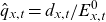 $\hat{q}_{x,t} = d_{x,t}/E_{x,t}^0$
. Similarly, central death rates can be estimated as
 $\hat{m}_{x,t} = d_{x,t}/E_{x,t}^c$
. Under the strict assumption of a constant force of mortality between both integer ages and calendar years, the force of mortality,
 $\mu_{x,t}$
, is equivalent to the central death rate,
 $m_{x,t}$
.
The death and central exposure data are assumed to be arranged in matrices
 $\boldsymbol{\mathit{D}} = (d_{x,t})$
and
 $\boldsymbol{\mathit{E^c}} = (E_{x,t}^c)$
, which are each
 $n_a \times n_y$
, so that we have
 $n_a$
ages,
 $n_y$
years, and
 $n_b = n_a + n_y - 1$
cohorts. Let
 $n = n_a n_y$
be the total number of observations. From these, the matrix
 $\boldsymbol{\mu} = (d_{x,t}/E_{x,t}^c)$
can be derived.
3. GAPC models
Mortality modelling and forecasting techniques can be broadly classified as being expectations-based, explanatory, or extrapolative in nature, with an overarching literature summary presented in Booth and Tickle (Reference Booth and Tickle2008). Amongst an actuarial readership, extrapolation has been favoured as the primary basis for mortality forecasting, with the most popular models decomposing mortality rates into a combination of age, period (or time), and cohort (or year of birth) effects. This decomposition allows the evolution of mortality rates to incorporate the effects of ageing, the effects of medical, nutritional, and social improvements over time, and the lifelong effects carried from an individual’s year of birth, arising from factors such as the implementation of nationwide healthcare and changing attitudes towards smoking (Li et al. Reference Li, Zhou and Hardy2015).
The literature on stochastic mortality models that exploit this age-period-cohort decomposition is vast. However, many authors have identified a number of similarities between these stochastic models, with Hunt and Blake (2021 b) defining them within a broad family known as GAPC models, which can be fitted using the R package StMoMo (Villegas et al. Reference Villegas, Kaishev and Millossovich2018). This draws upon the work of Currie (Reference Currie2016) that expresses these models within the standard terminology of generalised linear and non-linear models. By analogy, under the GAPC framework, a mortality model is comprised of four elements:
-
1. The random component: the numbers of deaths,
 $D_{x,t}$
, is random and is drawn from either a Poisson or a Binomial distribution: (3.1)
\begin{equation}D_{x,t} \sim \text{Poisson}(E_{x,t}^c \mu_{x,t}) \qquad \text{or} \qquad D_{x,t} \sim \text{Binomial}(E_{x,t}^0, q_{x,t}).\end{equation}
-
2. The systematic component: the predictor structure uses a linear or bilinear summation of a static age x effect
$\alpha_{x}$
, N random period factors
$\kappa_{t}^{(i)}$
,
$i=1,\ldots,N$
, and a random cohort factor
$\gamma_{t-x}$
, so that (3.2)where the age-modulating terms or factor loadings,
\begin{equation}\eta_{x,t} = \alpha_{x} + \sum_{i=1}^{N} \beta_{x}^{(i)} \kappa_{t}^{(i)} + {{\gamma_{t-x}}},\end{equation}
$\beta_{x}^{(i)}$
, can be either pre-specified functions of age,
$\beta_{x}^{(i)} \equiv f^{(i)}(x)$
, or non-parametric terms that need to be estimated.
-
3. The link function: the random and systematic components are linked using the canonical link function. For the Poisson distribution, the log link is used:
(3.3)and for the Binomial distribution, the logit link is adopted:
\begin{equation}\ln(\mu_{x,t}) = \eta_{x,t},\end{equation}
(3.4)
\begin{equation}\mathop{\mathrm{logit}}(q_{x,t}) = \eta_{x,t}.\end{equation}
-
4. The parameter constraints: in many situations, the estimated parameters can be transformed using arbitrary constants without changing
$\eta_{x,t}$
. Thus, to ensure identifiability of the models, various constraints may need to be imposed.


Many of the models in the actuarial literature can be defined within the GAPC framework in Equation (3.2), where the differences are derived entirely from the inclusion or exclusion of static age,
 $\alpha_x$
, and cohort,
 $\gamma_{t-x}$
, terms, the number of age-period factors, N, and the age-modulating functions being parametric,
 $f^{(i)}(x)$
, or non-parametric,
 $\beta_x^{(i)}$
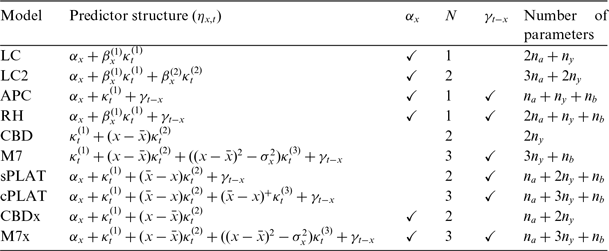
. This is summarised in Table 1, which indicates the main features of 10 common GAPC models. We briefly review these models in what follows and refer the reader to Hunt and Blake (Reference Hunt and Blake2021b) and Villegas et al. (Reference Villegas, Kaishev and Millossovich2018) for more comprehensive reviews.
Summary of existing GAPC models and their features. Here
 $\bar{x}$
is the average of the age range in the data,
 $\sigma_x^2$
is the variance of the age range in the data, and
 $(\bar{x}-x)^+=\max\{0, \bar{x}-x\}$
.

GAPC models rose to prominence via the revolutionary work of Lee and Carter (Reference Lee and Carter1992) which remains one of the most widely used projection models. The Lee–Carter (LC) model parsimoniously deconstructs the force of mortality into a bilinear summation of only age and period terms. The LC model can also be extended to larger numbers, N, of age-period factors (Hunt and Blake Reference Hunt and Blake2020b), such as the
 $N=2$
model by Renshaw and Haberman (Reference Renshaw and Haberman2003b), herein referred to as the Lee–Carter 2 (LC2) model. Renshaw and Haberman (Reference Renshaw and Haberman2006) further observe distinct ripple patterns when LC deviance residuals are plotted against cohorts, and thus propose the addition of a cohort term,
 $\gamma_{t-x}$
, to produce the Renshaw–Haberman (RH) model. The age-period-cohort (APC) model, obtained by setting
 $\beta_x^{1}=1$
in the RH model, is the classical age-period-cohort model which was introduced to the actuarial readership by Currie (Reference Currie2006), despite having a longer history in other fields (Holford Reference Holford1983).
Cairns et al. (Reference Cairns, Blake and Dowd2006) introduce the Cairns-Blake-Dowd (CBD) model which exploits the linearity of mortality rates on the log-scale at older ages. The CBD model can also be viewed as a variant of the LC model, with
 $N=2$
age-period terms and pre-specified age-modulating parameters
 $\beta_x^{(1)}\equiv f^{(1)}(x)=1$
and
 $\beta_x^{(2)}\equiv f^{(2)}(x)=x-\bar{x}$
. The lack of a static age term,
 $\alpha_x$
, does provide relative parsimony; however, this tends to restrict its usage to modelling higher ages. However, even across older ages, mortality rates are not strictly linear in age, and thus Cairns et al. (Reference Cairns, Blake, Dowd, Coughlan, Epstein, Ong and Balevich2010) propose the M7 model to incorporate cohort effects and an age-curvature term.
A particularly promising model, herein referred to as the cPLAT, is proposed in Plat (Reference Plat2009). This model includes the static age term from the LC model that is suitable for full age ranges, the cohort effect of the RH model that adheres well to historical data, and the multiple age-period factors provided by the CBD model. In this model, Plat (Reference Plat2009) includes a put option pay-off function,
 $f^{(3)}(x) = (\bar{x}-x)^+=\max\{0, \bar{x}-x\}$
, which means that
 $\kappa_t^{(3)}$
will have no effect on ages greater than
 $\bar{x}$
. This is to reflect the notion that lower ages tend to behave differently from higher ages due to factors such as traffic accidents and other external causes of death. Therefore, when modelling only higher ages, Plat (Reference Plat2009) simplifies the structure to define the sPLAT model. Similarly, Hunt and Blake (Reference Hunt and Blake2020b) and Dowd et al. (Reference Dowd, Cairns and Blake2020) recently consider extending the CBD and M7 models by adding an age effect,
 $\alpha_x$
, introducing the CBDx and M7x models.
3.1. Forecasting mortality with GAPC models
In the general setting of GAPC mortality models, the time evolution of mortality is determined by the period effects
 $\kappa_t^{(i)}$
,
 $i=1,\ldots,N$
, and the cohort effect
 $\gamma_{t-x}$
. To forecast mortality rates, the standard approach (Villegas et al. Reference Villegas, Kaishev and Millossovich2018) is to assume that the period indices follow a multivariate random walk so that
 \begin{equation}\boldsymbol{\kappa}_t = \boldsymbol{\delta} + \boldsymbol{\kappa}_{t-1} + \boldsymbol{\xi}_t^\kappa, \qquad \boldsymbol{\kappa}_t =\left(\! \begin{array}{c} \kappa_t^{(1)} \\ \vdots\\ \kappa_t^{(N)} \end{array} \!\right), \qquad \boldsymbol{\xi}_t^\kappa\sim N(\mathbf{0},\Sigma),\end{equation}
where
 $\boldsymbol{\delta}=\{\delta^{(1)},\ldots, \delta^{(N)}\}'$
is an N-dimension column vector of drift parameters and
 $\Sigma$
is the
 $N\times N$
variance–covariance matrix of the multivariate white noise
 $\boldsymbol{\xi}_t^\kappa$
. For the cohort effect, the standard approach is to assume that it follows a univariate ARIMA model:
 \begin{equation} {{\Delta^{d} \gamma_{c} = \delta_{0} + \sum_{k=1}^{p} \phi_{k} \Delta^{d} \gamma_{c-k} + \xi_{c} + \sum_{j=1}^{q} \delta_{j} \xi_{c-j}.}}\end{equation}
where
 $\Delta$
is the difference operator,
 $\phi_{k}$
are the autoregressive coefficients,
 $\delta_{j}$
are the moving average coefficients, and
 $\xi_{c}$
is a Gaussian white noise process with variance
 $\sigma_{\xi}^2$
.
Let
 $t_{n_y}$
denote the last year where mortality data are available. To obtain mortality projections for forecast horizon h, one first obtains period index forecasts
 $\hat{\boldsymbol{\kappa}}_{t_{n_y}+h}$
and, if necessary, a cohort index forecast
 $\hat{\gamma}_{t_y-x+h}$
using their respective time series models. The mortality projections at horizon h are then given by:
 \begin{equation}\skew{22}\widehat{\ln(\mu_{x,t_{n_y}+h})} = \hat{\alpha}_{x} + \sum_{i=1}^{N} \hat{\beta}_{x}^{(i)} \hat{\kappa}_{t_{n_y}+h}^{(i)} + \hat{\gamma}_{t_{n_y}-x+h}\end{equation}
or
 \begin{equation}\skew{30}\widehat{\mathop{\mathrm{logit}}(q_{x,t_{n_y}+h})} = \hat{\alpha}_{x} + \sum_{i=1}^{N} \hat{\beta}_{x}^{(i)} \hat{\kappa}_{t_{n_y}+h}^{(i)} + \hat{\gamma}_{t_{n_y}-x+h}.\end{equation}
4. Group regularisation for model construction
One limitation of the mortality modelling literature relates to the limited number of models that are considered when selecting the most appropriate model for a particular data set. In theory, there are an infinite number of models that can be produced within the GAPC framework, corresponding to every possible combination of terms:
 $\alpha_x$
, N,
 $\beta_x^{(i)}$
,
 $f^{(i)}(x)$
, and
 $\gamma_{t-x}$
, where
 $f^{(i)}(x)$
can take on various functional forms and parametrisations. Ideally, we would be able to consider every possible model; however, this is currently not feasible due to computational constraints, so we typically rely on a small subset of models. Importantly, it is perhaps unreasonable to expect that all data sets can be entirely explained by one of the 10 models summarised in Table 1. For example, a better fit for a particular data set may be obtained by adjusting the “strike” price of the put option pay-off in the cPLAT model to some
 $k \in \mathbb{Z}$
, or through an alternative functional form entirely.
To overcome these issues, we exploit regularisation techniques to propose a framework to construct bespoke GAPC mortality models for specific data sets by selecting appropriate age-modulating functions,
 $f^{(i)}(x)$
, from a large suite of basis functions. This resembles the data-driven framework proposed in Hunt and Blake (Reference Hunt and Blake2014); however, our approach is underpinned by regularisation and resampling approaches, which automatically determine the optimal degree of complexity for different applications by assessing how well a statistical model will generalise to unseen out-of-sample data (Hastie et al. Reference Hastie, Tibshirani and Friedman2001). With this, our approach makes more efficient use of data to draw statistical inferences and make predictions and places a stronger emphasis on out-of-sample performance for model selection.
4.1. Model framework
Whilst in the GAPC framework the number of deaths is assumed to be drawn from either a Poisson or Binomial distribution, we model the dependent variable,
 $\ln(D_{x,t}/E^c_{x,t})$
, as a Gaussian generalised linear model. This decision is made for computational efficiency, noting that closed-form solutions for group regularisation estimates exist when using ordinary least squares (Breheny and Huang Reference Breheny and Huang2015).
The main drawback of ordinary least squares estimation is that the errors are assumed to be homoscedastic. As noted by Brouhns et al. (Reference Brouhns, Denuit and Vermunt2002a), this is unrealistic as the logarithm of the observed force of mortality becomes much more variable at older ages due to the significantly smaller absolute number of deaths, which may have important consequences for inference and interval estimates of the model parameters (Brouhns et al. Reference Brouhns, Denuit and Vermunt2002b). Fortunately, for central parameter estimates and central predictions, the differences between the homoscedastic log-Gaussian approach and the heteroscedastic Poisson approach tend to be minimal (Brouhns et al. Reference Brouhns, Denuit and Vermunt2002a; Renshaw and Haberman Reference Renshaw and Haberman2003a).
Therefore, in the interest of computational efficiency, our general base model consists of the following modified version of the GAPC framework described in Equations (3.1)–(3.4):
-
1. The random component: the logarithm of the force of mortality follows a Normal distribution so that
(4.1)
\begin{equation}\ln(D_{x,t}/E^c_{x,t}) \sim \text{Normal}(\!\ln (\mu_{x,t}), \sigma^2).\end{equation}
-
2. The link function: the identity link (canonical) is used, such that
(4.2)
\begin{equation}\eta_{x,t} = g(E[\!\ln(D_{x,t}/E^c_{x,t})]) = \ln(\mu_{x,t}).\end{equation}
-
3. The systematic component: the predictor captures age, period, and cohort effects, using
(4.3)where the number of age-period terms, B, is very large. Here,
\begin{equation}\eta_{x,t} = \alpha_x + \sum_{i=1}^B f^{(i)}(x) \kappa_t^{(i)} + \gamma_{t-x},\end{equation}
-
−
$\boldsymbol{\alpha} = (\alpha_1,\ldots,\alpha_{n_a})$
is a row vector of coefficients to capture patterns by age; -
−
$\boldsymbol{\kappa^{\mathbf{(i)}}} = (\kappa_1^{(i)},\ldots,\kappa_{n_y}^{(i)})$
are row vectors of coefficients to capture systematic improvements over time; -
−
$f^{(i)}(x)$
are pre-defined functions to modulate trends by age; and -
−
$\boldsymbol{\gamma} = (\gamma_1,\ldots,\gamma_{n_b})$
is a row vector of coefficients to capture fixed effects embedded in years of birth.






Crucially, we include a large number, B, of age-period terms in the initial model specification, which allows the model to select from a wide range of potential trends.
Footnote 1
This is done through the specification of the different factor loadings,
 $f^{(i)}(x)$
, which modulate how the random period factors,
 $\kappa^{(i)}_t$
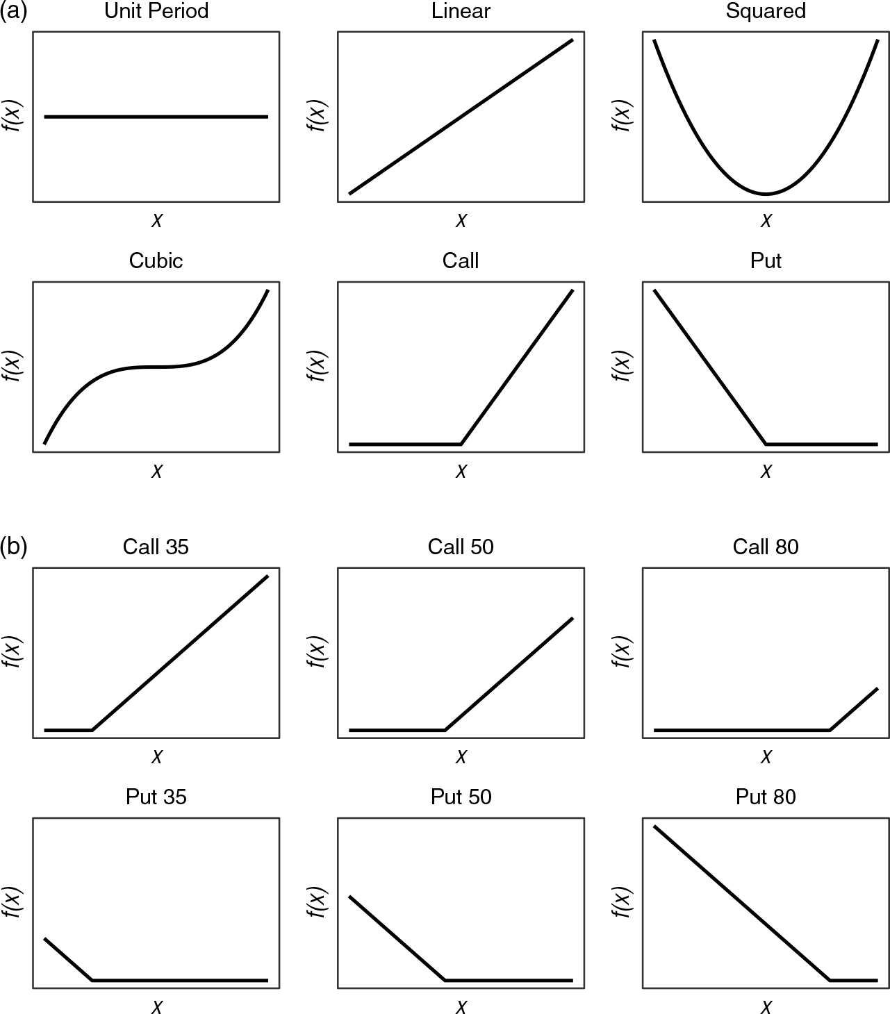
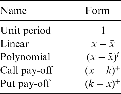
, impact different ages to determine how the age-period mortality curve changes through time. As a starting point, we consider five different continuous functional forms for
 $f^{(i)}(x)$
, which are summarised in Table 2 and illustrated in Figure 1(a). Within each functional form, we also consider various parametrisations, as illustrated in Figure 1(b).
Examples of age-modulating basis functions,
 $f^{(i)}(x)$
, included in initial group regularisation model specification (a) by type, and (b) by parametrisation (for call and put option pay-offs).

Basis functions,
 $f^{(i)}(x)$
, included in initial group regularisation model specification.

The unit period term determines the general level of mortality and is included to capture systematic improvements over time that affect all ages equally, arising from increasing social advances (Cairns et al. Reference Cairns, Blake and Dowd2006). The linear or slope term, however, could capture the recent trend towards an increasing concentration of deaths around the mean age of death, known as “rectangularisation” (Biffis Reference Biffis2005). Further, the inclusion of higher-order polynomials is inspired by the curvature in
 $\mathop{\mathrm{logit}}(q_{x,t})$
plots, mirroring various extensions to the CBD model (Li and O’Hare Reference Li and O’Hare2017; Cairns et al. Reference Cairns, Blake, Dowd, Coughlan, Epstein, Ong and Balevich2010). Similarly, the call and put option pay-offs are motivated by the cPLAT model (Plat Reference Plat2009); however, we consider a greater range of strikes. We note that the framework and its associated implementation are flexible enough to allow the consideration of other functional forms beyond those in Table 1. For example, we could also consider the parametric forms in the “Age Function” toolkit of Hunt and Blake (Reference Hunt and Blake2014), orthogonal piecewise linear splines as in Aro and Pennanen (Reference Aro and Pennanen2011), Wavelets as in Hainaut and Denuit (Reference Hainaut and Denuit2020), or B-Splines (Currie et al. Reference Currie, Durban and Eilers2004). We explore the use of this latter type of basis function in our empirical exercise in Sections 5 and 6.
4.2. Model identifiability
As with most GAPC models, parameter identifiability might be a concern, especially given the diversity of basis functions allowed within the initial model (see Hunt and Blake, Reference Hunt and Blake2020a,b and Currie Reference Currie2020 for a detailed discussion on this matter). For example, we can freely move the general level of mortality across the age, period, and cohort parameters through the transformations:
 \begin{equation}\left(\alpha_x, \kappa^{(i)}_t\right)\to\left(\alpha_x + b_if^{(i)}(x), \kappa^{(1)}_t - b_i\right), \quad \text{$i =1,\ldots, B$},\end{equation}
and
 \begin{equation}\left(\alpha_x, \gamma_{t-x}\right)\to\left(\alpha_x + b, \gamma_{t-x} - b\right)\!,\end{equation}
for b and
 $b_i$
,
 $i =1,\ldots, B$
, arbitrary constants. Thus, we set
 $\kappa_{1}^{(i)}=0$
,
 $i=1,\ldots, B$
so that
 $\alpha_x$
can be interpreted as the age shape of mortality in the first year of the data. Similarly, we set
 $\gamma_{1}=0$
.
Besides the shifting of mortality levels, Hunt and Blake (Reference Hunt and Blake2020a) show that if a GAPC model contains basis functions spanning polynomials up to order
 $M-1$
, then the model possesses invariant transformations which allow the arbitrary movement of polynomial trends of order M across the age, period, and cohort parameters. However, we do not impose any explicit parameter constrains to deal with such invariant transformations, noting that we mitigate the possible impact of this identifiability issue on projections by modelling both the period and cohort indices using time series models with an order of integration
 $d=1$
. As discussed in Currie (Reference Currie2020), such a choice of the order of integration implies that in most situations, the forecast mortality rate values would be invariant despite the possible non-identifiability of the model parameters. Moreover, the empirical evidence suggests that mortality rates across most ages and many countries have unit roots and are difference stationary, justifying the use of
 $d=1$
(Njenga and Sherris Reference Njenga and Sherris2011).
Footnote 2
4.3. Generalised linear model representation
Leveraging the result from Currie (Reference Currie2016), we can express the systematic component as a generalised linear model. Let
 $\boldsymbol{\eta} = \text{vec}(\!\ln(\boldsymbol{\mu}))$
; here, the vec operator stacks the columns of a matrix in column order on top of each other, so
 $\boldsymbol{\eta}$
is column vector of dimensions
 $n\times1$
with
 $n=n_an_y$
. We can then write Equation (4.3) in matrix form:
 \begin{equation}\boldsymbol{\eta} = \boldsymbol{X} \boldsymbol{\beta} = \sum_{j=0}^{B+1} \boldsymbol{X}_j \boldsymbol{\beta}_j,\end{equation}
where the coefficients vector,
 $\boldsymbol{\beta}$
, can be decomposed into
 $B+2$
non-overlapping groups:
 \begin{equation}\boldsymbol{\beta} = (\boldsymbol{\beta_0}', \text{ } \boldsymbol{\beta_1}', \text{ } \boldsymbol{\beta_2}', \text{ } \ldots \text{ } , \text{ } \boldsymbol{\beta_B}', \text{ } \boldsymbol{\beta_{B+1}}')' = (\boldsymbol{\alpha}, \text{ } \boldsymbol{\kappa^{(1)}}, \text{ } \boldsymbol{\kappa^{(2)}}, \text{ } \ldots \text{ } , \text{ } \boldsymbol{\kappa^{(B)}}, \text{ } \boldsymbol{\gamma})'.\end{equation}
The first group refers to the vector of static age coefficients,
 $\boldsymbol{\alpha}$
. The next B groups denote each set period of period coefficients,
 $\boldsymbol{\kappa^{(i)}}$
,
 $i=1,\ldots, B$
, while the final group denotes the vector of cohort coefficients,
 $\boldsymbol{\gamma}$
. The design matrix,
 $\boldsymbol{X}$
, can also be divided:
 \begin{equation}\boldsymbol{X} = [\boldsymbol{X_0}:\boldsymbol{X_1}:\boldsymbol{X_2}: \ldots : \boldsymbol{X_B}: \boldsymbol{X_{B+1}}],\end{equation}
where
 $\boldsymbol{X}_j$
refers to the portion of the design matrix related to the predictors in Group j. For example, the first portion,
 $\boldsymbol{X_0}$
 $(n \times n_a)$
, defines the design matrix corresponding to
 $\boldsymbol{\alpha}$
. Similarly,
 $\boldsymbol{X_i}$
 $(n \times n_y)$
defines each
 $\boldsymbol{\kappa^{(i)}}$
for
 $i = 1,2,...,B$
, and
 $\boldsymbol{X_{B+1}}$
 $(n \times n_b)$
defines
 $\boldsymbol{\gamma}$
.
4.4. Group regularisation fitting
Typically, to estimate parameters in GAPC-style models,
 $\boldsymbol{\hat\beta} = (\boldsymbol{\hat\alpha}, \text{ } \boldsymbol{\hat\kappa^{(1)}},$
 $ \text{ } \boldsymbol{\hat\kappa^{(2)}}, \text{ } \ldots \text{ }, \text{ } \boldsymbol{\hat\kappa^{(B)}}, \text{ } \boldsymbol{\hat\gamma})'$
, we maximise the log-likelihood or minimise the residual sum of squares. These will estimate all the coefficients in the model, noting that all values will likely be non-zero. Whilst suitable for existing pre-defined GAPC models, these approaches are not appropriate for our framework. If every estimated coefficient from our model were nonzero, we would have a highly over-parametrised and complex model with
 $n_a + B\times n_y + n_b$
parameters. This would be problematic due to interpretability and predictive accuracy, commonly referred to as the “
 $p>n$
” problem (James et al. Reference James, Witen, Hastie and Tibshirani2013).
Instead, we estimate parameters using group regularisation (Yuan and Lin Reference Yuan and Lin2006; Breheny and Huang Reference Breheny and Huang2015), which minimises the objective function:
 \begin{equation}Q(\boldsymbol{\beta}|\boldsymbol{X}, \boldsymbol{\eta}) = L(\boldsymbol{\beta}|\boldsymbol{X}, \boldsymbol{\eta}) + \sum_{j=1}^{B+1} p_{\lambda}(\lVert \boldsymbol{\beta_j} \rVert),\end{equation}
where
 $L(\boldsymbol{\beta}|\boldsymbol{X}, \boldsymbol{\eta})$
denotes the residual sum of squares, and
 $p_{\lambda}(\cdot)$
is a penalty function applied to the Euclidean (
 $\ell_2$
) norm of each group to prevent the model from becoming too complex.
The key result is that the penalty function carries out group selection, meaning that within a group, coefficients will either all be zero or all be non-zero: if Group j is selected, then
 $\hat\beta_{jk} \ne 0$
for all k, and otherwise
 $\hat\beta_{jk} = 0$
for all k. For example, if Group 1 is not selected,
 $\hat\kappa_t^{(1)}$
will be zero for all t, and the age-period pair
 $f^{(1)}(x)\kappa_t^{(1)}$
will be eliminated from the model. Therefore, this estimation approach will select basis functions from the initial large model to best capture the period and cohort patterns in each data set.
There are alternative ways of defining the penalty function,
 $p_{\lambda}(\cdot)$
, including the group lasso penalty (Yuan and Lin Reference Yuan and Lin2006), the smoothly clipped absolute deviation penalty (Fan and Li Reference Fan and Li2001), and the minimax concave penalty (Zhang Reference Zhang2010). We have decided to use the minimax concave penalty (MCP),
 \begin{equation}p_{\lambda, \gamma}(\theta) =\begin{cases}\lambda \theta - \frac{\theta^2}{2\nu}, & \text{if } \theta \leq \nu \lambda, \\[4pt]\frac{1}{2} \nu \lambda^2, & \text{if } \theta > \nu \lambda,\end{cases}\end{equation}
which is a function of the tuning parameter,
 $\nu$
, and the penalty term,
 $\lambda$
. The MCP not only selects which groups of basis function to include but also shrinks estimated coefficients to prevent the model from over-fitting to noise, and thus each unique
 $(\nu, \lambda)$
defines a unique fitted model. However, for ease of computation, we fix the tuning parameter to be
 $\nu = 3$
, which aligns with common practice (Breheny and Huang Reference Breheny and Huang2015). Thus,
 $\lambda$
solely controls the trade-off between goodness of fit and parsimony; the larger the value of
 $\lambda$
, the heavier the penalisation, resulting in a more parsimonious model (fewer included basis functions and smaller estimated coefficients).
It is worth noting that the objective function in Equation (4.9) depends on the original scale of the design matrix
 $\boldsymbol{X}$
, which in turn depends on the original scale of the basis functions
 $f^{(i)}(\cdot)$
,
 $i=1,\ldots,B$
. To abstract from the original scale of the basis functions, the group-specific design matrices
 $\boldsymbol{X_j}$
,
 $j=1,\ldots,B+1$
, are orthonormalised prior to fitting and then transformed back to the original scale after fitting the model (Breheny and Huang Reference Breheny and Huang2015).
4.5. Block cross-validation for
$\lambda$
selection

The value of
 $\lambda$
in the group regularisation defines a regularisation path containing GAPC mortality models with varying levels of complexity among which we need to choose the model considered best for a given application. To determine the optimal degree of penalisation, we propose a block cross-validation-style approach (Racine Reference Racine2000; Bergmeir and Benitez Reference Bergmeir and Bentez2012; Bergmeir et al. Reference Bergmeir, Costantini and Bentez2014) that aims to assess how well a model is likely to perform over a given forecasting horizon. This approach, which is in the spirit of the resampling methods discussed in Atance and DebÓn (Reference Atance and DebÓn2020), involves iteratively dividing the in-sample data into training data to fit the models and test data to assess forecasting abilities.
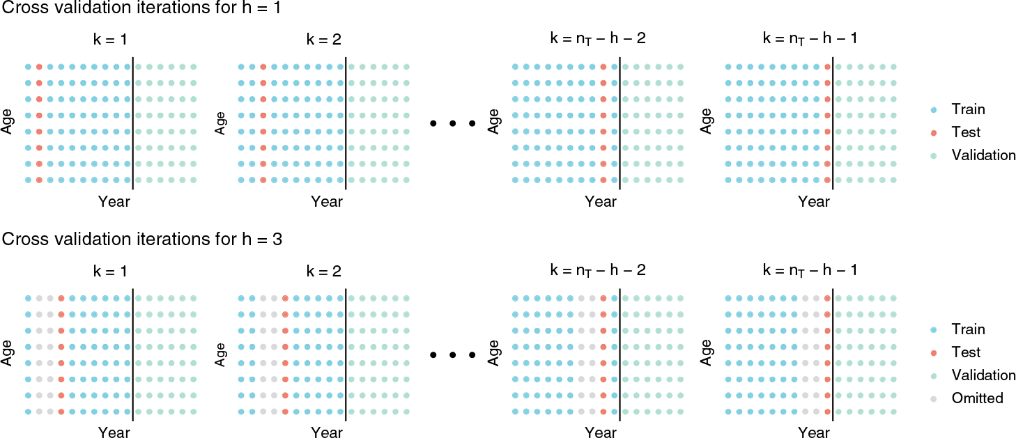
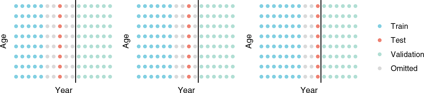
First, a portion of the data (roughly one-third) at the end is held back for validation, denoted as
 $\mathcal{V}$
and shown by the green points in Figure 2. This corresponds to time periods
 $t = n_T+1, n_T+2, \ldots , n_T+n_E$
. The remaining data (
 $t = 1, 2, \ldots , n_T$
) are used for training and testing, where the test sets can take different widths to reflect differing forecasting horizons, as illustrated in Figure 2. For example, to select a model to forecast a 1-year horizon, test sets are defined as 1-year blocks (top row of Figure 2), whereas by contrast, to select a model to forecast a 3-year horizon, test sets are defined as 3-year blocks (bottom row of Figure 2). Therefore, the training sets (blue) for forecasting horizon h are defined as:
 \begin{equation}\mathcal{T}^k(h) = \{(x,t)\}_{t \notin [k+1, k+h]},\end{equation}
Iterations of cross-validation for horizon
 $h=1$
(top row) and
 $h=3$
(bottom row). for all
 $k = 1, 2, ..., n_T-h-2,n_T-h-1$
.

and the test sets (red) as:
 \begin{equation}\mathcal{F}^k(h) = \{(x,t)\}_{t = k+h},\end{equation}
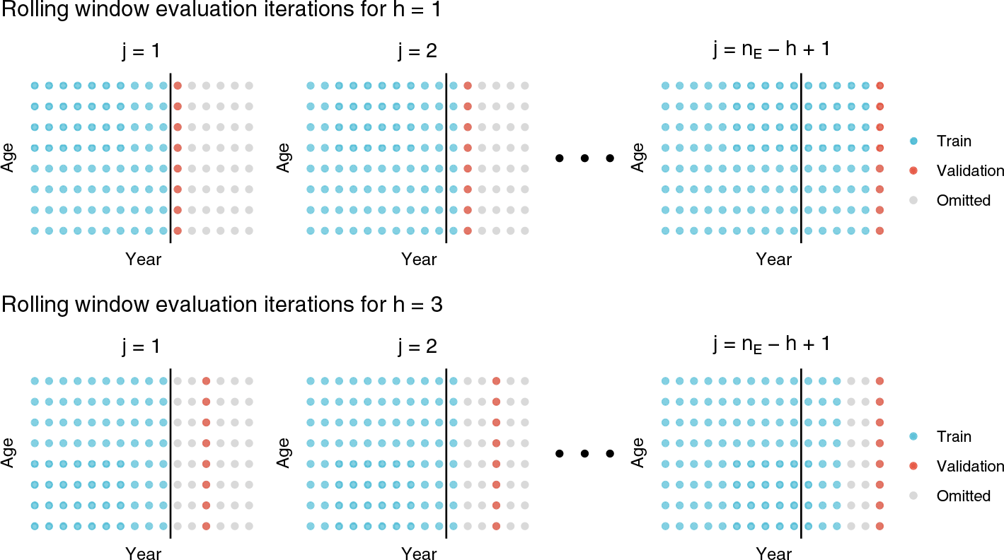
Inspired by Bergmeir et al. (Reference Bergmeir, Hyndman and Koo2018), we use data both to the left and right of each test set to train the model, which contrasts heavily to the more common rolling window out-of-sample evaluation illustrated in Figure 3 (Tashman Reference Tashman2000; Dowd et al. Reference Dowd, Cairns, Blake, Coughlan, Epstein and Khalaf-Allah2009). This allows us to conduct significantly more test sets for a given data set than if we were restricted to fitting models using only data to the left, since this would place a limit on how far to the left test sets can occur. Moreover, we also minimise the portion of data that is left completely unused (grey), thereby extracting as much information as possible and producing an error estimate that is less variable than that of the traditional out-of-sample procedure (Bergmeir et al. Reference Bergmeir, Costantini and Bentez2014).
Iterations of a rolling window approach for horizon
 $h=3$
.

Given that every training set will contain at least one observation from every age (row) and cohort (major diagonal) of the data set, the full vector of coefficients will be produced for the age,
 $\boldsymbol{\hat{\alpha}}$
, and cohort,
 $\boldsymbol{\hat{\gamma}}$
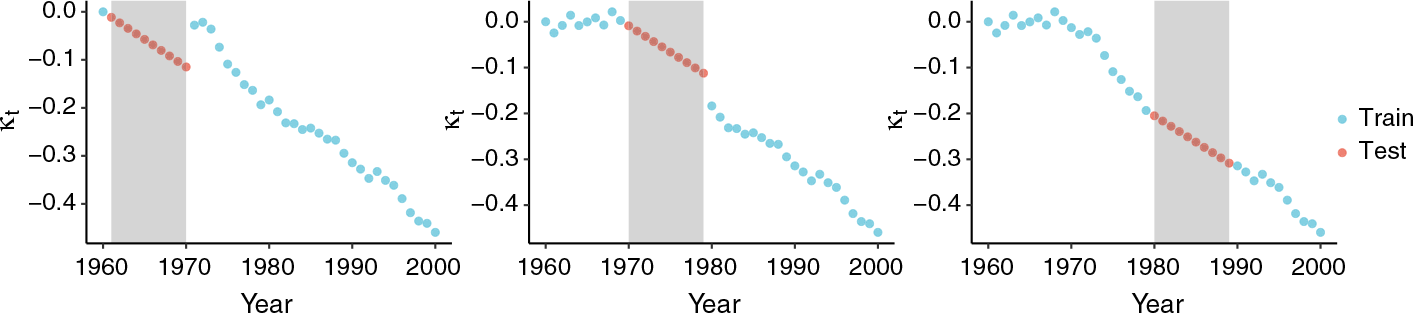
, terms. In other words, we will be able to estimate a coefficient corresponding to every age group and to every cohort. However, there will not be any observations from the non-training years, and thus all
 $\boldsymbol{\hat{\kappa}^{(i)}}$
will not be estimated fully. Figure 4 illustrates three examples, where the blue circles correspond to
 $\hat\kappa_t^{(i)}$
values that can be estimated directly from the training data, and the grey shaded regions to non-training years. Therefore, in order to assess the ability of a model to predict the test sets, we need to impute the missing values. This is achieved by fitting a random walk with drift using all the period indices that are observable (blue circles), both to the left and right of the missing region:
 \begin{equation}\kappa_t^{(i)} = \kappa_{t-1}^{(i)} + \delta^{(i)} + \epsilon_t^{(i)},\end{equation}
where
 $\epsilon_t^{(i)}$
is a Gaussian white noise process and
 ${\delta}^{(i)}$
is the drift. We can then predict the red circles using a forward fill procedure, basing predictions on the value from the previous period:
 \begin{equation}\hat{\kappa}_t^{(i)} = \hat{\kappa}_{t-1}^{(i)} + \hat{\delta}^{(i)}.\end{equation}
With these estimates, we can then compute the fitted/predicted values:
 \begin{equation}\widehat{\ln(\mu_{x,t})} = \hat{\alpha}_x + \sum_{i=1}^B f^{(i)}(x) \hat{\kappa}_t^{(i)} + \hat{\gamma}_{t-x},\end{equation}
and the mean squared error (MSE) for the test set:
 \begin{equation}\text{CV}_k(h) = \frac{1}{n_a} \sum_{(x,t) \in \mathcal{F}^k(h)} \left(\widehat{\ln\left(\mu_{x,t}\right)}-\ln\left(\mu_{x,t}\right)\right)^2.\end{equation}
This procedure is iterated for all test sets,
 $\mathcal{F}^k(h)$
,
 $k = 1, 2, ..., n_T-h-2,n_T-h-1$
, to determine the cross-validation error at horizon h:
 \begin{equation}\text{CV}(h) = \frac{1}{n_T-h-1} \sum_{k=1}^{n_T-h-1} \text{CV}_k(h).\end{equation}
This approach can be used to compare between a number of models and to select the “optimal” model that has the lowest cross-validation error for forecasting horizon h. This includes being able to test a grid of penalties,
 $\boldsymbol{\Lambda} = \{\lambda_\ell\}_{\ell=1}^{L}$
, in our group regularisation approach to select, for every horizon
 $h=1,\ldots,H$
, the value which minimises this error:
 \begin{equation}\hat{\lambda}(h) = \mathop{\mathrm{argmin}}_{\lambda \in \boldsymbol{\Lambda}} \text{CV}(h;\,\lambda).\end{equation}
Illustration of time series imputation approach. The blue points correspond to
 $\hat\kappa_t$
estimates that can be estimated directly from the training set, and the grey area to the non-training years that cannot be estimated with the red points indicating the values imputed using a forward fill procedure.

4.6. Rolling window model evaluation
After selection, we must then evaluate our chosen model using completely independent and unseen data to ensure that it performs competitively relative to its peers. We implement out-of-sample evaluations with a rolling window approach, akin to Dowd et al. (Reference Dowd, Cairns, Blake, Coughlan, Epstein and Khalaf-Allah2009), using the validation data,
 $\mathcal{V}$
.
As shown in Figure 5, we fit the models using all in-sample data (blue) and forecast on the unseen validation set (red), which we assume contains
 $n_E$
years. We then roll forward one period
 $n_E-h$
times until all data are exhausted. Similar to the cross-validation procedure, forecasting is enabled by extrapolating the period and cohort parameters over the required time horizon, with a difference being that this is now achieved using conventional time series forecasting as discussed in Section 3.1. The out-of-sample MSEs at horizon h for each validation set can then be computed, using
 \begin{equation}\text{MSE}_j(h) = \frac{1}{n_a} \sum_{(x,t) \in \mathcal{V}^j(h)} \left(\widehat{\ln(\mu_{x,t})}-\ln(\mu_{x,t})\right)^2,\end{equation}
where
 $\mathcal{V}^j(h)= \{(x,t)\}_{t = n_T+j+h-1}$
for
 $j=1,\ldots,n_E-h+1$
. The overall out-of-sample MSE at horizon h is then given by:
 \begin{equation}\text{MSE}(h) = \frac{1}{n_E-h+1} \sum_{j=1}^{n_E-h+1} \text{MSE}_j(h).\end{equation}
Iterations of rolling window out-of-sample evaluation for horizon
 $h=1$
(top row) and
 $h=3$
(bottom row).

In the cross-validation and evaluation of models, we follow Booth et al. (Reference Booth, Hyndman, Tickle and de Jong2006) and focus on the log-rates when assessing model accuracy. This is to reduce the impact of older ages which would otherwise dominate model selection and comparison due to the exponential increase in mortality rates with age. Moreover, without the log-transformation, older ages can distort model comparison due to their higher mortality uncertainty. However, it is noted that Equations (4.16) and (4.19) can readily be adapted to focus on errors on the untransformed mortality rates or errors in life expectancies.
5. Illustration using data for US males
In this section, we illustrate the proposed group regularisation (GR) construction framework using US males mortality data obtained from the HMD. We focus on modelling adult age ranges, 20–89 years, using years 1960–2000 as our in-sample data, and years 2001–2017 as our validation set.
5.1. Initial basis functions
To implement the GR framework, we consider a base model with
 $B=37$
basis functions taken from the functional forms in Table 1 as follows:
 \begin{align}f^{(1)}(x) &= 1; \end{align}
 \begin{align}f^{(2)}(x) &= x - \bar{x}; \end{align}
 \begin{align}f^{(2+j)}(x) &= (x - \bar{x})^{j+1}, \quad j=1,\dots,9; \end{align}
 \begin{align}f^{(11+r)}(x) &= (x - 20 - 5r)^+, \quad r=1,\dots,13; \end{align}
 \begin{align}f^{(24+p)}(x) &= (20 + 5p - x)^+, \quad p=1,\dots,13. \end{align}
5.2. Regularisation path
To search for the optimal level of regularisation, we consider a grid of 25 values of
 $\lambda$
equally spaced on the log-scale and in the range
 $\left[e^{-9},e^{-3.5}\right]$
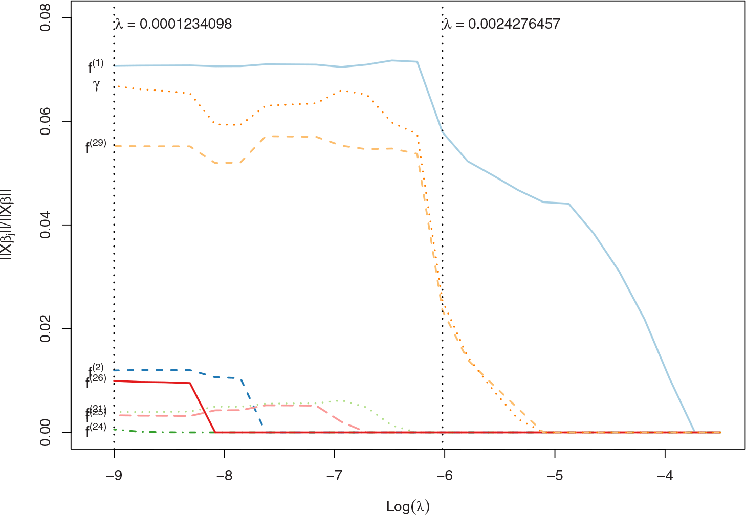
. This range is wide enough to produce a regularisation path which starts with a very over-parametrised model and ends in a very parsimonious model. The resulting regularisation path is shown in Figure 6, which shows the relative size of each Group j of coefficients
 $\lVert \boldsymbol{\mathit{{X}_{j}}} \boldsymbol{\beta}_j\rVert/\lVert\boldsymbol{\mathit{X}} \boldsymbol{\beta}\rVert$
as a function of
 $\ln(\lambda)$
. In this particular exercise, we have decided not to penalise the
 $\boldsymbol{\alpha}$
parameters so that the model always contains a static age term
 $\alpha_x$
, independent of the amount of regularisation. This is because we are considering the age range 20 to 89 years, where the static age term is always believed to be important to appropriately capture the accident hump at younger ages (Plat Reference Plat2009; Hunt and Blake 2021 b).
Regularisation path of mortality models for US males fitted to age range of 20–89 years for years 1960–2000.

Small values of
 $\lambda$
correspond to low levels of regularisation and more complex models. As such, to the left of Figure 5 when
 $\lambda=0.0001234098$
, we start with the model:
 \begin{equation}\begin{split}\ln(\mu_{x,t}) = \alpha_x + \kappa_t^{(1)} + (\bar{x}-x) \kappa_t^{(2)} + (x-70)^+ \kappa_t^{(21)} + (x-85)^+ \kappa_t^{(24)} + \\ (25-x)^+ \kappa_t^{(25)} + (30-x)^+ \kappa_t^{(26)} +(45-x)^+ \kappa_t^{(29)} + \gamma_{c},\end{split}\end{equation}
which, in addition to the default static age term and the cohort effect, includes 7 of the 37 possible age-period terms. Noticeably, this very complex model includes terms that capture the idiosyncrasies of mortality trends and noise at very young and very old ages via the
 $\kappa_t^{(21)}$
,
 $\kappa_t^{(24)}$
,
 $\kappa_t^{(25)}$
, and
 $\kappa_t^{(26)}$
terms. As we increase the value of
 $\lambda$
, the additional regularisation induces the elimination of some age-period terms, resulting in more parsimonious models. For example, when we reach a value of
 $\lambda=0.0024276457$
, we obtain the model:
 \begin{equation}\ln(\mu_{x,t}) = \alpha_x + \kappa_t^{(1)} + (45-x)^+ \kappa_t^{(29)} + \gamma_{c},\end{equation}
which, as opposed to the seven age-period terms of the initial model, only includes two age-period terms capturing the general level of mortality and the differential improvement of individuals younger than 45 years of age. We note that this model is very similar to the sPLAT model, albeit without the linear term and with the strike of the put function at 45 rather than
 $\bar{x}=54.5$
.
5.3. Selected values of
$\lambda$

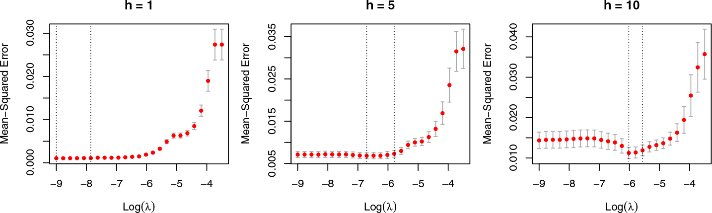
Given the regularisation path, the next step is to select a model suitable for each forecasting horizon using the block cross-validation approach described in Subsection 4.5. The selected
 $\hat\lambda(h)$
for each horizon h is the value that minimises the cross-validation MSE. Figure 7 illustrates this for horizons
 $h=1, 5,$
and 10, where the selected values correspond to
 $\hat\lambda(1) = 0.0001234098$
,
 $\hat\lambda(5) = 0.001220697$
, and
 $\hat\lambda(10) = 0.0024276457$
, respectively. Note, for
 $\lambda$
values to the right of each respective
 $\hat\lambda$
, we have under-fitting, whilst to the left, we have over-fitting. Table 3 presents the selected
 $\hat\lambda(h)$
for all horizons of interest along with a summary of the corresponding model structure.
Cross-validation MSE for forecasting horizons
 $h=1$
,
 $h=5$
, and
 $h=10$
for US males data fitted to ages 20–89 years for years 1960–2000.

Summary of optimal model structures for group regurlarisation for ages 20–89 years in the period 1960–2000 in US males.

In the case of 1-year and 2-year forecasting horizons, the selected model has seven age-period terms and corresponds to the specification in Equation (5.6). This contrasts with the 7 to 10-year forecasting horizons for which the selected model corresponds to the simpler structure in Equation (5.7), which has only two age-period terms. In general, as indicated by Table 3, the longer the forecasting horizon, the higher the value of
 $\hat\lambda(h)$
, the fewer the number of period terms, and the more parsimonious the selected model specification.
5.4. Out-of-sample evaluation
Having selected appropriate models for each horizon, we now evaluate their out-of-sample performance relative to existing GAPC models using the rolling window approach described in Section 4.6, with validation data from 2001 to 2017. Thus, for horizon
 $h=1$
, there are 17 years for evaluation, which reduces to 8 years for horizon
 $h=10$
namely, 2010, 2011,
 $\dots$
, 2017, whose forecasts are derived using the years 2000, 2001,
 $\dots$
, 2007, as the last training year, respectively.
In the evaluation exercise, we consider two versions of the GR framework obtained by varying the number and form of the initial basis functions. The first version, herein referred to as GR1, corresponds to the implementation described previously in Subsection 5.1 which uses the
 $B=37$
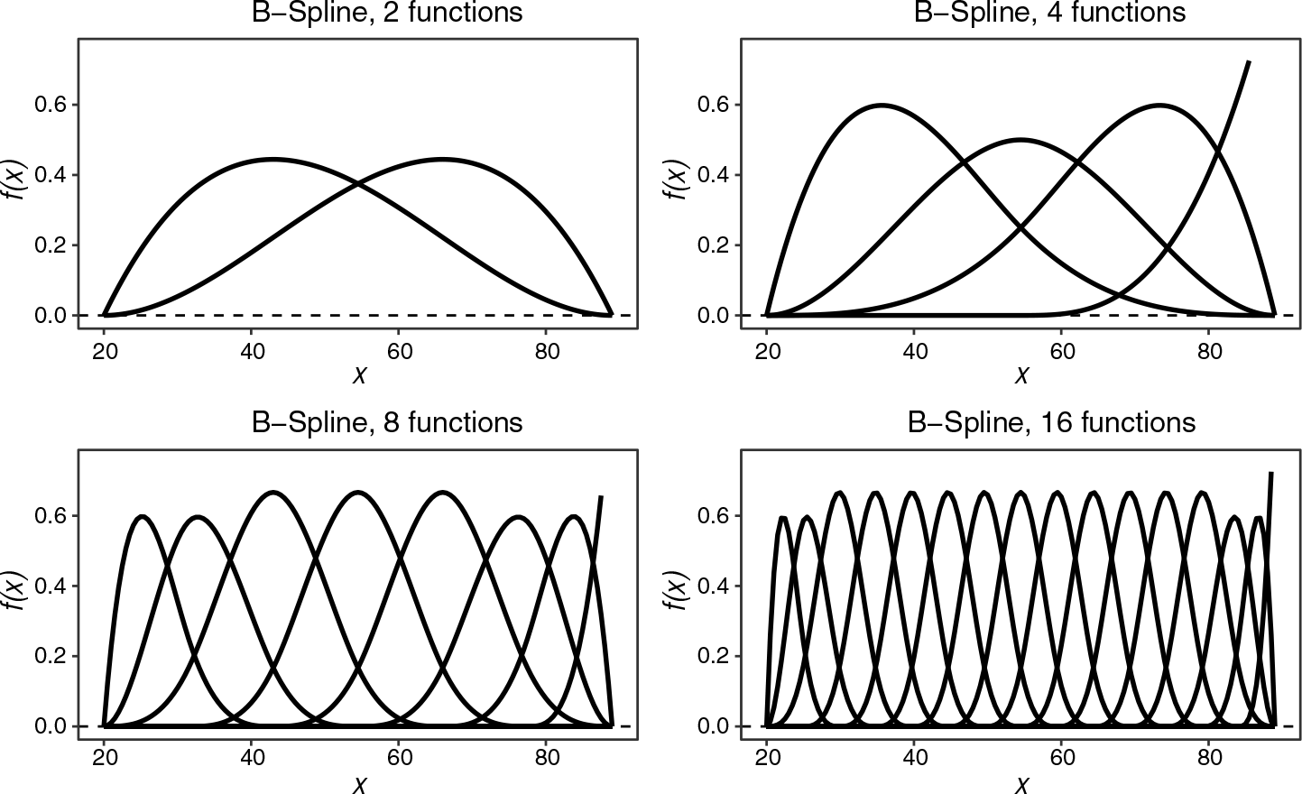
basis functions in Equations (5.1)–(5.5). The second version, referred to as GR2, explores the use of a larger pool of initial basis functions in order to enrich the types of trends that the model can capture. To do so, in addition to the 37 basis functions in Equations (5.1)–(5.5), we consider additional cubic B-Splines basis functions (Currie et al. Reference Currie, Durban and Eilers2004), which are piecewise polynomials commonly used in the graduation and forecasting of mortality (Macdonald et al. Reference Macdonald, Richards and Currie2018). Figure 8 depicts the basis functions we add, which are comprised of four groups of B-splines, each of which contain 2, 4, 8, and 16 functions, respectively. Thus, the total number of basis in the initial model under the GR2 implementation is
 $B=37+2+4+8+16=67$
.
Cubic B-splines basis functions added to the initial model for the GR2 version of the group regularisation implementation.

We consider as benchmarks eight of the ten GAPC models presented in Table 1. We have discarded the CBD and M7 models as they are both designed to fit higher ages (typically 50 years of age and beyond), and thus are not entirely appropriate for the 20–89 years age range considered in our experiments. While we estimate our regularised models using ordinary least squares under a log-Gaussian setting, we estimate all the classical GAPC models using maximum likelihood under a log-Poisson setting. This conforms with the existing literature that favours the use of a generalised (non-)linear framework for estimating GAPC models (Hunt and Blake Reference Hunt and Blake2021b). Appendix A includes the constraints used to ensure the identifiability of these benchmark models.
For the forecasting of the period functions in GAPC and GR models, we follow the standard approach and use a multivariate random walk with drift (Cairns et al. Reference Cairns, Blake, Dowd, Coughlan, Epstein, Ong and Balevich2010; Haberman and Renshaw Reference Haberman and Renshaw2011; Villegas et al. Reference Villegas, Kaishev and Millossovich2018). In addition, for models with a cohort effect, we forecast
 $\gamma_{t-x}$
using an ARIMA model as in Equation (3.6) with level of differentiation
 $d=1$
, autoregressive order
 $p=1$
, and moving average order
 $q=0$
. As discussed before in Subsection 4, choosing
 $d=1$
tempers the possible impact of model identifiability on projections (Currie Reference Currie2020). Moreover, setting
 $p=1$
is in line with the level autoregression found by others when modelling cohort effects (Cairns et al. (Reference Cairns, Blake, Dowd, Coughlan, Epstein and Khalaf-Allah2008); Cairns et al. (Reference Cairns, Blake, Dowd, Coughlan, Epstein and Khalaf-Allah2011); Hunt and Blake (2021 a)).
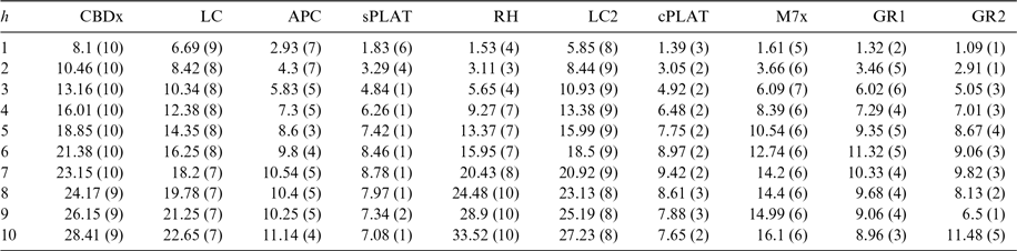
Table 4 presents the out-of-sample MSE by forecasting horizon for each of the eight GAPC models and the two implementations of the GR framework. Among the standard GAPC models, the sPLAT and cPLAT model have the best forecasting performance at every horizon, with the sPLAT model topping the ranking at 7 of the 10 forecasting horizons.
Out-of-Sample Mean Square Error for US males by forecasting horizon with model ranking in brackets. Values are presented as
 $1000 \times$
MSE.

The GR models perform competitively, outperforming the CBDx, LC, LC2, and M7x models at every horizon and the APC and RH at most horizons. Moreover, the GR approaches show a very consistent performance across all horizons, with MSE values which are very close to the MSE values of the sPLAT and cPLAT models. This is not surprising in the case of GR1, as for the US male data set for horizons
 $h=7, 8, 9, 10$
, the GR1 approach identified a model which closely resembles the cPLAT model (recall Equation (5.7)).
It is worth noting that for horizons 1 and 2, the GR2 approach outperforms all nine other competing models by a significant margin. By including the 67 additional basis functions depicted in Figure 8, the GR2 model can explore more complex models that are able to better capture the cross-sectional patterns in the mortality data. Hence, the improved performance of the GR2 over the rest of the models highlights the benefits of allowing for a larger variety of age-specific trends and complexity of model when conducting short-term mortality forecasts. However, this extra complexity comes at the cost of ease of interpretability of coefficients relative to the GR1 models.
6. Application to 52 data sets from the HMD
To further explore the proposed GR model construction framework, in this section, we apply this approach to 52 different empirical data sets from the HMD, corresponding to 26 countries and 2 genders. At the time of writing, the HMD had detailed mortality data for 41 countries or areas. The years of data vary by country, with only 28 countries or areas having data for the standardised period 1960–2017. Of the 28 remaining countries, we discard Iceland and Luxembourg as they have multiple data cells with 0 deaths, leaving us with 26 countries. Similar to the previous US male data example, we use the years 1960–2000 as our in-sample data and reserve the years 2001–2017 for out-of-sample evaluation.
6.1. Summary of model structures
The results of applying the GR approach reveal that the optimal model varies not only by country, but also within country, depending on the forecasting horizon. To illustrate this, Tables 5 and 6 report, respectively, the average characteristics of the model structures produced by the GR1 and GR2 approaches for different horizons.
Summary of optimal model structures according to GR1 for ages 20–89 years in the period 1960–2000 in 52 data sets.

Summary of optimal model structures according to GR2 for ages 20–89 years in the period 1960–2000 in 52 data sets.

Notably, across all 52 data sets,
 $\hat\lambda(h)$
tends to increase with the horizon of interest, which means that simpler models are constructed for longer forecasting periods. For example, while at horizon 1 the models have on average 4.77 and 6.98 period terms for GR1 and GR2, respectivley, at horizon 10, the average number of period terms reduces to 2.27 and 3.29. These results conform with the hypothesis of parsimony being preferred for longer horizons (Green and Armstrong 2015). More specifically, for shorter forecasting horizons, the predictive success of a model is determined by its ability to accurately fit the cross section of the mortality curve. By contrast, as the forecasting horizon increases, it becomes more important to filter out the year-on-year noise in the data, and having a closer fit to the initial mortality curve becomes less relevant.
It is also worth noting that the longer the horizon, the less likely the optimal structure will include a cohort effect. While at short horizons the optimal structure will almost certainly include a cohort effect, at horizon 10, only 60% of the 52 data sets will have a cohort effect under the GR1 approach. This proportion is further reduced to 35% under the GR2 approach, indicating that in the GR1 approach, the cohort effect might be acting as a substitute for uncaptured age-period trends.
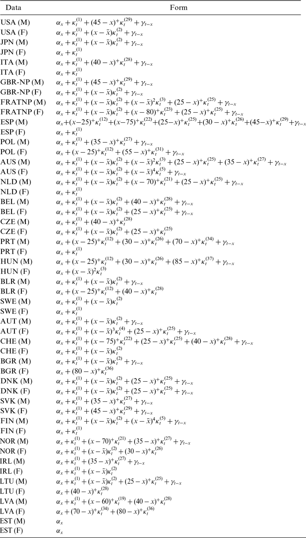
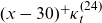
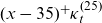
As an illustration of the diversity of models produced by the GR framework, Table 7 shows the optimal model produced by the GR1 approach at forecasting horizon 10 for all 52 data sets. In some cases, the optimal models are similar in structure to existing GAPC models. For example, for US females, Japanese males, UK (GBR-NP) females, Belarusian males, Austrian males, and Bulgarian males, the structure of the optimal model is the same as the sPLAT model. Similarly, for Swedish males, Czech females, and Irish females, the optimal model structure coincides with the CBDx model. In most cases, though, the optimal models vary quite remarkably from existing models, but with the following commonalities in the type of basis functions used for the different countries:
-
79% of models contain a unit period term,
$\kappa_t^{(1)}$
, which captures changes in the general level of mortality that affect all ages. -
42% of models contain a linear term,
$(x-\bar{x})\kappa_t^{(2)}$
which captures changes in the slope of the mortality curve. -
Only 6% of models contain a quadratic term,
$(x-\bar{x})^2\kappa_t^{(3)}$
, which captures the curvature of the mortality curve. -
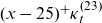
37% of models contain at least one of the terms,
$(x-25)^+\kappa_t^{(23)}$
,
$(x-30)^+\kappa_t^{(24)}$
, or
$(x-35)^+\kappa_t^{(25)}$
, which specifically target declining mortality rates at ages below 35 years, known as the “flattening of the accident hump.”


Optimal model structures according to GR1 for 10-year forecasting horizon using data for ages 20–89 years in the period 1960–2000.

Existing GAPC models are unable to capture the right combination of the above findings, stressing the merits of our data-driven approach and the pitfalls of using pre-defined structures for all data sets.
6.2. Out-of-sample evaluation
Whilst the previous section implies that a wide range of bespoke models may be more appropriate to explain historical data, it is important to assess whether the GR-constructed models generalise well out-of-sample and if they perform competitively relative to existing GAPC models. For the 52 data sets, we replicate the out-of-sample evaluation described in Section 5.4.
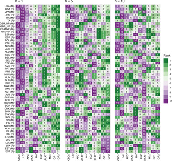
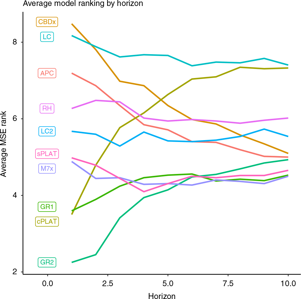
Figure 9 presents heatmaps reporting the ranking of the eight GAPC models and the two GR approaches for forecasting horizons
 $h=1, 5,$
and 10. In this figure, the GAPC models are ordered in terms of their complexity as indicated by their number of parameters. Similarly, the countries are ordered according to their population size. To facilitate the interpretation of these model rankings, Figure 10 presents the mean ranking of each of the 12 models as a function of the 10 forecasting horizons of interest.
Ranking of models according to out-of-sample MSE at
 $h=1$
,
 $h=5$
, and
 $h=10$
, for different data sets.

Average of out-of-sample MSE rank across all 52 data sets for each model.

Over the 1-year horizon, the GR2 approach produces the best result with a median rank of 2 and is in the top three models in 41 of the 52 data sets. Interestingly, the best performance of the GR2 approach is among the countries with the biggest populations. The GR1 approach also has a very strong performance at short horizons, surpassing most GAPC models, but is almost always outperformed by the GR2 approach. This reiterates the benefit of allowing for a larger variety of age-specific trends when focusing on short-term forecasting so that the cross-sectional variability of the mortality curve is better captured. The cPLAT and M7x models are the two best-performing GAPC models, particularly for larger populations, whilst the more parsimonious CBDx, APC, and LC models perform relatively poorly. This again reaffirms our hypothesis that complex models are preferred for shorter horizons and for less noisy data sets.
As we increase the forecasting horizon, the absolute values of the forecasting errors increase for all models, as would be expected. However, the relative rankings of the models also change, which is of far more interest. The strong performance of our GR approaches remain consistent, with the GR1 in particular having the best median rank at horizons 5 and 10, reflecting the ability of our regularisation approach to filter out the year-on-year noise in the mortality trends to produce a parsimonious model which concentrates on the secular longer-term trends. Footnote 3 In contrast, the other models show a significant shift, with more parsimonious models, such as the APC and the CBDx, now performing significantly better than the complex cPLAT, M7x, and LC2 models. This notion of simplicity outperforming complexity over longer horizons is further supported by the improving performance of the GR1 models relative to GR2 as h increases.
Interestingly, the popular cPLAT and LC models rank within the bottom four models almost exclusively for the longer horizons. Notably, one of the only data sets where the cPLAT model performs reasonably well over a 10-year horizon is for the US populations, which is actually the data that Plat (Reference Plat2009) used to construct this model. This lends support to the notion that if we examine data and build a model based on the patterns observed within it, as Plat (Reference Plat2009) did for the USA, we can expect to yield strong forecasting results. However, we cannot just assume that a model that explains US mortality well will fit well to all other countries. Thus, we must repeat this procedure for each data set, which is effectively what our data-driven approach aims to do.
7. Simulation study
To validate the findings from the preceding section in a more robust manner, we consider the use of simulated data sets. These are created by first simulating mortality rates from a specific GAPC model, and subsequently sampling the number of deaths from a Poisson distribution to reflect random variation, with the simulation process described in detail in Appendix B. This framework provides a controlled setting to isolate and understand specific effects, namely (a) the complexity of the underlying process from which mortality rates are generated, (b) the population size from which deaths are sampled (or level of noise), and (c) the length of the forecasting horizon. For each of the following subsections, we systematically vary one of these three elements and use as a reference example for comparison the case where rates are generated from an APC model, using a population size of 5 million to predict rates at a forecasting horizon of 10 years. For each combination of inputs, we run 100 simulations. Footnote 4 For this section, the RH, LC2, and GR2 models are not considered due to being computationally taxing.
7.1. Effect of generator model
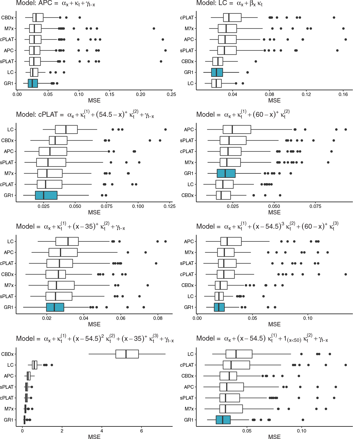
Figure 11 illustrates forecasting errors using data generated by a number of GAPC models, including models defined in the literature (APC, LC, and cPLAT), and others that have been randomly constructed using a suite of basis functions. These models have been created to reflect varying numbers of age-period terms, the inclusion/exclusion of a cohort term, and a range of basis functions with different forms and parametrisations. This includes a basis function not considered in the GR approach in the bottom right panel, namely a unit period term applying to ages 50 years and below only.
Boxplot of mean squared errors from 100 simulated data sets, involving (a) rates generated from different GAPC models, (b) using a population size of 5 million, and (c) a forecasting horizon of 10 years.

As expected, in the first three panels, the model that generated each data set performs very well with regard to both median errors and the range of errors across the 100 simulations. However, the performance of models on data generated from another model is of far greater interest. Notably, no single GAPC model performs strongly across all scenarios, with the complex models, such as the cPLAT and M7x, tending to perform stronger on the more complex data sets, and more parsimonious models, such as the LC and APC, performing better on the simpler data sets. More strikingly, this study highlights the significance of the cohort term, where models without a cohort term perform extremely poorly where cohort effects are prevalent in the underlying data. This is most pronounced in the bottom left panel of Figure 11, where the LC and CBDx models generate unwieldy errors.
By contrast, the GR1 model performs strongly and consistently, with the lowest median error in six of the eight scenarios, and ranking within the top three models every time. This is hardly surprising, given the adaptability of its framework to select more period and/or cohort terms where more complex patterns exist in the underlying data.
7.2. Effect of population size
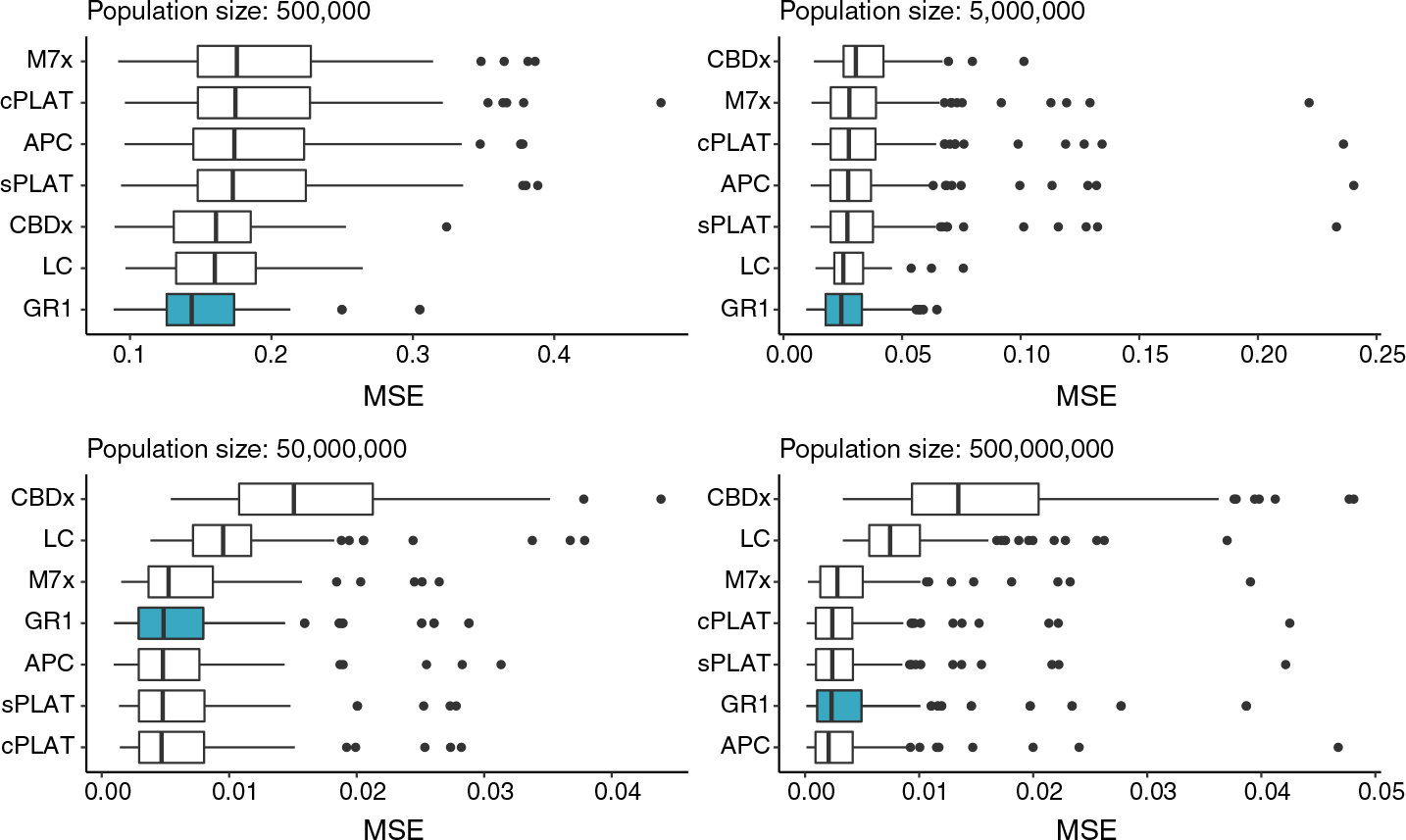
When population size decreases (or the level of noise increases), it is obvious that forecasting errors will increase in absolute terms, as illustrated in Figure 12. However, the changes in the relative performance of the models are more insightful. For very small populations, complex models have a tendency to overfit the Poisson noise in the data, resulting in a poor forecasting performance, with higher median forecasting errors and increased tendencies to produce significantly large errors or anomalies. In contrast, the more parsimonious LC and CBDx models perform stably for these smaller populations as their reduced number of parameters allows them to better filter the Poisson noise.
Boxplot of mean squared errors from 100 simulated data sets, involving (a) rates generated from an APC model, (b) using varying population sizes, and (c) a forecasting horizon of 10 years.

The GR1 model, however, remains competitive under all scenarios, registering the lowest median error on the 500,000 and 5 million populations, and recording extremely similar median errors to the best models for the larger 50 and 500 million populations. Notably, in all scenarios, the GR1 approach tends to select a model structure that is similar to or exactly matches that of the APC model that generated the data, which explains the strikingly similar results of these two models for larger populations. Interestingly, however, the GR1 model significantly outperforms the APC model for the smaller populations, which owes to the ability of the regularisation approach to not only select basis functions but also to shrink parameter estimates to avoid over-fitting to noise in the training data.
7.3. Effect of forecasting horizon
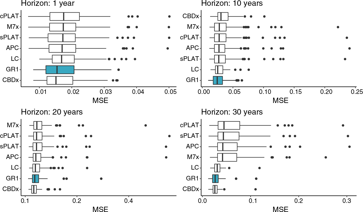
Figure 13 illustrates errors for varying forecasting horizons, where for consistency, the number of years of training data was amended in each scenario such that the GR1 approach had 30 test sets per horizon. For the short-term 1-year horizon, all models perform strongly in absolute terms, with similar median errors observed for all models. However, even for this horizon, it is observed that there is a greater tendency for the complex models such as the cPLAT, M7x, and sPLAT to produce large, unwieldy errors, owing to the potential to overfit to noise given the large number of parameters. This poor and volatile performance of the complex models is even more pronounced as the length of the forecasting horizon increases, where there is a noticeable difference between the two simplest GAPC models – CBDx and LC – and the others. This mirrors the behaviour observed in Section 6. For all horizons, the GR1 approach performs strongly, which again owes to the ability to simplify the underlying structure of the model as the forecasting horizon increases.
Boxplot of mean squared errors from 100 simulated data sets, involving (a) rates generated from an APC model, (b) using a population size of 5 million, and (c) varying forecasting horizons.

8. Conclusions
In this paper, we have introduced and applied a data-driven framework to construct bespoke GAPC mortality models, which has been made available in an open-source R package StMoMo. Our approach considers a large suite of parametric functions, which users can modify based on their views of “demographic significance,” to best capture patterns in specific data sets. The procedure is fitted using group regularisation and cross-validation techniques to determine the optimal trade-off between complexity and parsimony for each data set and application, which includes both selecting which basis functions to include in the final model and determining how heavily to shrink the estimated coefficients to prevent over-fitting.
Our exhaustive empirical analysis revealed that no pre-defined model can perform well for every data set and application, and thus our regularised data-driven models are superior to existing models on average. Moreover, our empirical analysis revealed an interesting divide between simple and complex models, with parsimonious models outperforming as forecasting horizons increase and population sizes decrease. This link between parsimony and forecasting performance was particularly noticeable at shorter forecasting horizons where allowing for more complex age-specific trends proved to significantly improve the forecasting performance of GAPC models.
However, it is important to stress that while our model construction approach is mostly data-driven, subjectivity is still inherent to any modelling exercise, requiring input from the modeller at several steps of the modelling process. In our framework, the user needs to decide on the quantity and form of the initial basis functions, the historical length of data used for model training and testing, and the specific criterion for model selection. Therefore, it is important to stress that the key contribution of this paper is neither the models nor the rankings generated, but rather the framework that we have introduced. We simply aim to complement the toolkit available to modellers by providing an alternative approach to thinking about mortality modelling through the lens of statistical learning techniques.
We fitted our models using an ordinary least squares setting for computational efficiency. However, in an actuarial context, GAPC models are traditionally fitted under a Poisson or Binomial framework which facilitates the appropriate measurement of all sources of uncertainty when deriving interval estimates of mortality rates, life expectancies, and annuity values (Brouhns et al. Reference Brouhns, Denuit and Vermunt2002b). In such situations, one can use the log-Gaussian approach proposed in this paper as a screening tool to identify the model structure that is better suited for a particular data set. Then, given this model structure, model parameters can be re-estimated under a Poisson framework. However, we do aim to develop a Poisson-fitting framework, taking advantage of emerging computational tools for fitting regularised generalised linear models, such as the smurf package (Devriendt et al. Reference Devriendt, Antonio, Reynkens and Verbelen2020). Furthermore, future research may also consider the use of more complex time series models for the period indices, such as ARIMA(p,d,q) models. Accordingly, the construction framework could be extended to not only select the optimal basis functions but also the optimal time series specification of the period terms.
Finally, we have only used the MSE of the log-mortality rates for model selection and evaluation. However, this can be adapted to other criteria, such as errors in survival probabilities, life expectancies, or implied annuity prices. Further, in many financial applications, forecast intervals are of greater interest than point estimates. Therefore, future research may consider interval-based measures, such as interval scorecards, which count the number of times the realised mortality rate falls within a confidence range (Gneiting and Raftery Reference Gneiting and Raftery2007).
Acknowledgements
This research is funded by Society of Actuaries Center of Actuarial Excellence 2016 Research Grant on Longevity Risk and the Australian Research Council Centre of Excellence in Population Ageing Research (CEPAR) project number CE110001029.
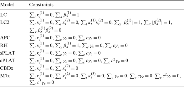
Appendix A. Identifiability Constraints for GAPC Models
Table A.1. shows the constraints we use to identify the eight GAPC models tested in the paper. For LC, LC2, and CBDx, we follow the approach discussed in Hunt and Blake (Reference Hunt and Blake2020b), while for APC, sPLAT, cPLAT, and M7x we follow Hunt and Blake (Reference Hunt and Blake2020a). For the RH model, we impose the constraints suggested by Hunt and Villegas (Reference Hunt and Villegas2015) in order to improve the stability and robustness of the model.
Identifiability constraints for GAPC models.

Appendix B. Simulating Data Sets
The simulation of the data sets in Section 7 involves first simulating mortality rates from a specific GAPC model and then randomly generating the number of deaths from a Poisson distribution to reflect sampling variation, or noise. For illustration, here we outline a seven-step procedure to simulate data from the APC model: B
 \begin{equation}\eta_{x,t} = \ln({\mu_{x,t}}) = \alpha_x + \kappa_t + \gamma_c;\end{equation}
however, this procedure can be extended and applied to any GAPC model.
Step 1: Generate reasonable estimates for
 $\boldsymbol{\alpha}$
,
 $\boldsymbol{\kappa}$
, and
 $\boldsymbol{\gamma}$
.
We first need to fit the generator model, from which mortality rates can be simulated. This is achieved by fitting an APC model to US female data for the years 1960–2017, ages 20–89 years, and cohorts 1871–1997. Using the Poisson maximum likelihood approach embedded in the R package StMoMo by Hunt and Villegas (Reference Hunt and Villegas2015), we can estimate
 \begin{equation}\boldsymbol{\hat\alpha} = (\hat\alpha_{{{20}}}, \ldots, \hat\alpha_{89}), \qquad \boldsymbol{\hat\kappa} = (\hat\kappa_{1960}, \ldots, \hat\kappa_{2017}), \qquad \boldsymbol{\hat\gamma} = (\hat\gamma_{1871}, \ldots, \hat\gamma_{1997}).\end{equation}
Step 2: Fit time series models to
 $\boldsymbol\kappa$
and
 $\boldsymbol\gamma$
.
The simulation of mortality rates requires the projection of the period index,
 $\boldsymbol{\kappa}$
, and cohort index,
 $\boldsymbol{\gamma}$
. We assume that each follows a univariate random walk with drift:
 \begin{equation}\kappa_t = \kappa_{t-1} + \delta_0 + \epsilon_t \qquad \text{and} \qquad \gamma_c = \gamma_{c-1} + \delta_1 + \varepsilon_c,\end{equation}
where
 $\epsilon_t$
and
 $\varepsilon_c$
are Gaussian white noise processes with variance
 $\sigma_{\epsilon}^2$
and
 $\sigma_{\varepsilon}^2$
, respectively. With these models, we can simply and easily estimate
 $\hat\delta_0$
and
 $\hat\delta_1$
.
Step 3: Simulate
 $\boldsymbol\kappa$
and
 $\boldsymbol\gamma$
over a 100-year horizon.
From the fitted time series models, we can then simulate values of the period index,
 $\dot{\kappa}_{2017+s}$
, and the cohort index,
 $\dot{\gamma}_{1997+s}$
, over the next 100 years (
 $s=1, \ldots, 100$
):
 \begin{equation}\dot\kappa_{2017+s} = \hat\kappa_{2017} + s\hat\delta_0 + \sum_{t=1}^s \epsilon_t \qquad \text{and} \qquad \dot\gamma_{1997+s} = \hat\gamma_{1997} + s\hat\delta_1 + \sum_{c=1}^s \varepsilon_c.\end{equation}
Step 4: Simulate mortality rates,
 $\dot{\mu}_{x,t}$
, for 100-year horizon.
With this, we can calculate the associated value of the predictor over the 100-year horizon:
 \begin{equation}\dot{\eta}_{x,{{2017}}+s} = {{\hat\alpha_x + \dot{\kappa}_{{{2017}}+s} + \dot{\gamma}_{{{2017}}+s-x}.}}\end{equation}
These can then be converted into the age-specific forces of mortality (rates),
 $\dot{\mu}_{x,{{2017}}+s}$
, by inverting the canonical log-link function:
 \begin{equation}\dot{\mu}_{x,{{2017}}+s} = e^{\dot{\eta}_{x,{{2017}}+s}}.\end{equation}
Step 5: Generate exposure matrix,
 $\boldsymbol{E^c}$
.
For simplicity, we assume that the exposure is time-invariant,
 $E_{x,t}^c \equiv E_{x}^c$
. Therefore,
 $\boldsymbol{E^c}$
has 100 columns, each of which are identical. We assume that the age structure mirrors the observed exposures for the US females in 2017, given by
 $E_{x,2017}^c$
. Therefore
 \begin{equation}E_{x}^c = p \times \frac{E_{x,2017}^c}{\sum_{x} E_{x,2017}^c},\end{equation}
where p denotes the total population size being simulated.
Step 6: Generate death count matrix,
 $\boldsymbol{D}$
.
We then produce the matrix of death observations using the simulated central mortality rates by randomly drawing from a Poisson distribution:
 \begin{equation}D_{x,{{2017}}+s} \sim \text{Poisson}(E_{x}^c \dot{\mu}_{x,{{2017}}+s}).\end{equation}
Step 7: Repeat procedure 100 times for the given combination of generator model and population.
Appendix C. Group Regularisation in StMoMo
We have implemented the model construction framework introduced in this paper as an extension of the R package StMoMo (Villegas et al. Reference Villegas, Kaishev and Millossovich2018). The implementation of the group regularised fitting is underpinned by the use of the R package grepreg (Breheny and Huang Reference Breheny and Huang2015) which provides fast and stable group descent algorithms for general group regularisation purposes. In this Appendix, we illustrate the replication of some of the results associated with the US males example presented in Section 5.
Currently, the group regularisation functions are available in the GroupLasso branch of the development version of StMoMo, available in Github at https://github.com/amvillegas/StMoMo/tree/GroupLasso. This branch will be integrated to the CRAN version of the package after publication of this paper. The GroupLasso development version can be installed with the following commands:
install.packages("devtools")
devtools::install_github("amvillegas/StMoMo", ref = "GroupLasso")
The code below defines a base model with the
 $B=37$
basis functions in Equations (5.1)–(5.5):
library(StMoMo)
strikes <- seq(25, 85, 5)
baseModel <- StMoMo(
link = "log-Gaussian",
staticAgeFun = TRUE,
periodAgeFun = c("1", genPoly(1:10), genCall(strikes),
genPut(strikes)),
cohortAgeFun = "1"
)
The genPoly, genCall, and genPut functions are utility functions to generate, respectively, basis functions,
 $f^{(i)}(x)$
, of polynomial form (Equation (5.3)), call pay-offs (Equation (5.4)), and put pay-offs (Equation (5.5)). There is also the genSpline utility function to generate B-Spline basis such as those depicted in Figure 8.
To fit the models to US male data, we need to download these data from the Human Mortality Database. This can be done using the package demography (Hyndman et al. Reference Hyndman, Booth, Tickle and Maindonald2017) with the code:
library(demography)
USAdata <- hmd.mx(country = "USA", username = username,
password = password)
dataStMoMo <- StMoMoData(USAdata, series = "male")
dataStMoMo$Dxt <- round(dataStMoMo$Dxt)
The username and password above are for the Human Mortality Database and should be replaced appropriately.
The main function for fitting a regularisation path is grpfit. We can use this function to fit the regularisation path induced by a grid of 25 values of
 $\lambda$
in the range
 $\left[e^{-9},e^{-3.5}\right]$
applied to data for the period 1960–2000 and the age range 20–89 years:
lambda <- exp(seq(-3.5, -9, length.out = 25))
GRfit <- grpfit(
baseModel,
lambda = lambda,
data = dataStMoMo,
ages.fit = 20:89,
years.fit = 1960:2000)
We can then plot the regularisation path as follows:
plot(GRfit, lwd = 2)

The cross-validation framework described in Section 4.5 is implemented in function cv.grpStMoMo. For example, to select an appropriate level of regularisation for forecasting horizon
 $h=10$
, we can use function cv.grpStMoMo as follows:
GRCV_10 <- cv.grpStMoMo(
baseModel,
h = 10,
lambda = lambda,
data = dataStMoMo,
ages.train = 20:89,
years.train = 1960:2000
)
Since cross-validation entails repeated refitting of the models, the above code can take a couple of minutes to run. We can then plot the cross-validation error as a function of
 $\lambda$
with the code:
plot(GRCV_10)

The value of
 $\lambda$
with the minimum cross-validation error is reported in GRCV_10$lambda.min and the corresponding index within the grid is reported in GRCV_10$min. This index can be used in combination with function extractStMoMo to extract the model that minimises the cross-validation error at horizon
 $h=10$
:
GRfit_10 <- extractStMoMo(GR1fit, k = GRCV_10$min)
The output of extractStMoMo is a standard StMoMo object which can be used with the standard functions of StMoMo such as plot, fitted, forecast, and simulate. For example, we can plot the selected model for horizon
 $h=10$
as follows:
plot(GRfit_10, nCol = 4)