1 Introduction
The unique features of patterned surfaces and porous coatings have long been recognized (e.g. Marmur Reference Marmur2004). Of particular interest are coupled flows and transport processes through and above permeable and/or (micro-) patterned layers, as they are ubiquitous in environmental, biological and engineered systems. Examples of natural systems include transport in fractured rocks and flows over sediment beds (Nikora et al. Reference Nikora, Goring, McEwan and Griffiths2001; Goharzadeh, Khalili & Jørgensen Reference Goharzadeh, Khalili and Jørgensen2005; Battiato & Vollmer Reference Battiato and Vollmer2012; Liu et al. Reference Liu, Shang, Kerisit, Zachara and Zhu2013), coral reefs and canopies (Nepf et al. Reference Nepf, Ghisalberti, White and Murphy2007; Ghisalberti Reference Ghisalberti2009; Papke & Battiato Reference Papke and Battiato2013; Battiato & Rubol Reference Battiato and Rubol2014), nutrient uptake from roots (Marschner & Dell Reference Marschner and Dell1994; Gilroy & Jones Reference Gilroy and Jones2000) and passive predatory strategies in some carnivorous plants (Lloyd et al. Reference Lloyd1942; Goharzadeh et al. Reference Goharzadeh, Khalili and Jørgensen2005; Scholz et al. Reference Scholz, Bückins, Dolge, Erlinghagen, Weth, Hischen, Mayer, Hoffmann, Riederer and Riedel2010). Coupled flows are critical to many engineering applications including superhydrophobic (Ou, Perot & Rothstein Reference Ou, Perot and Rothstein2004; Rothstein Reference Rothstein2010; Battiato Reference Battiato2014) and slippery liquid-infused porous surfaces (Cui et al. Reference Cui, Daniel, Grinthal, Lin and Aizenberg2015; Hou et al. Reference Hou, Hu, Grinthal, Khan and Aizenberg2015), shear sensors, flows in blood vessels (Weinbaum et al. Reference Weinbaum, Zhang, Han, Vink and Cowin2003; Al-Chidiac et al. Reference Al-Chidiac, Mirbod, Andreopoulos and Weinbaum2009) and above carbon nanotube forests (Deck et al. Reference Deck, Ni, Vecchio and Bandaru2009; Battiato, Bandaru & Tartakovsky Reference Battiato, Bandaru and Tartakovsky2010; Battiato Reference Battiato2012), just to mention a few. Distinctive characteristics of microstructured surfaces and nanoimprints are routinely adopted in a variety of other manufacturing processes including, but not limited to, ultrafiltration of colloids (Maruf et al. Reference Maruf, Wang, Greenberg, Pellegrino and Ding2013b ) and nutrient delivery in bioreactor devices (Griffiths, Howell & Shipley Reference Griffiths, Howell and Shipley2013; Gruenberger et al. Reference Gruenberger, Probst, Heyer, Wiechert, Frunzke and Kohlheyer2013). Channel transverse mixing is critical to, e.g., reduce membrane fouling or increase the overall reactivity of a system. This is particularly challenging in microfluidic devices where mixing is controlled by diffusion, with resulting slow reaction rates. Surface patterns have been successfully employed to enhance transverse mixing in microchannels (Stroock et al. Reference Stroock, Dertinger, Ajdari, Mezic, Stone and Whitesides2002; Stroock & Whitesides Reference Stroock and Whitesides2003) and reduce membrane fouling (Weinman & Husson Reference Weinman and Husson2016). Yet, a clear connection between the properties of the surface and its macroscopic response still remains an open question (Bouquet & Lauga Reference Bouquet and Lauga2011). Notwithstanding significant theoretical advancements, attempts to relate surface properties to macroscopic quantities, such as the dispersion coefficient and average velocity, remain mostly phenomenological (e.g. Li, Reinhoudt & Crego-Calama Reference Li, Reinhoudt and Crego-Calama2007; Ybert et al. Reference Ybert, Barentin, Cottin-Bizonne, Joseph and Bocquet2007; Maruf et al. Reference Maruf, Rickman, Wang, Mersch, Greenberg, Pellegrino and Ding2013a ; Hou et al. Reference Hou, Hu, Grinthal, Khan and Aizenberg2015), and analytical expressions are available only for tractable geometries (e.g. Lauga & Stone Reference Lauga and Stone2003; Davis & Lauga Reference Davis and Lauga2010).
Here, we consider non-reactive tracer transport through a symmetric (micro-)channel embedded in a permeable porous matrix, and characterize the latter by its permeability and porosity. In this work, we are concerned with analytically relating the macroscopic response of the coupled channel–matrix system, i.e. the longitudinal dispersion coefficient, with the porous layer porosity and permeability and the channel transport regimes. We assume that the flow and transport are governed by the combination of Stokes, Brinkman and advection–diffusion equations subject to appropriate initial and boundary conditions. This formulation, relevant for the study and control of transverse mixing in microchannels, is especially suitable for the modelling of Navier–Stokes flows (both laminar and turbulent) above patterned surfaces, e.g. micro-riblets (Battiato Reference Battiato2014) and carbon nanotube forests (Battiato et al. Reference Battiato, Bandaru and Tartakovsky2010; Battiato Reference Battiato2012), where the idealization of the pattern as a porous layer has been shown to be appropriate.
Two approaches are routinely employed to relate channel and matrix properties to dispersion in a coupled channel–matrix system: (i) analytical and semianalytical solutions of a system of coupled advection–diffusion equations (ADEs) and (ii) upscaling perturbative methods. While exact, analytical solutions of a system of ADEs can often be obtained only under restrictive simplifying assumptions. The greatest technical difficulty in (semi)analytically solving advection–diffusion equations is in accounting for the non-uniformity of the velocity profile in the channel and/or matrix. This complication is generally overcome, or better avoided, by assuming uniform velocity in the channel, purely diffusive transport in the matrix or both. The first analytical treatment of transport mechanisms in channel–matrix systems is generally attributed to Tang, Frind & Sudicky (Reference Tang, Frind and Sudicky1981), who considered a one-dimensional thin channel embedded in an impermeable (to flow) porous matrix. Their result was later extended by Sudicky & Frind (Reference Sudicky and Frind1982) to account for the presence of neighbouring parallel channels. A detailed review of this approach is provided by Bodin, Delay & De Marsily (Reference Bodin, Delay and De Marsily2003). More recently, Roubinet, Dreuzy & Tartakovsky (Reference Roubinet, Dreuzy and Tartakovsky2012) solved semi-analytically the transport problem for a uniform flow in a two-dimensional channel embedded in an impermeable two-dimensional infinite matrix, where mass transport was purely diffusive.
Alternative approaches to connect macroscale transport properties to surface properties are upscaling methods, such as homogenization (Hornung Reference Hornung1997; Boso & Battiato Reference Boso and Battiato2013), volume averaging (Whitaker Reference Whitaker1999), thermodynamically constrained averaging (Gray & Miller Reference Gray and Miller2005), stochastic homogenization, the method of moments (Brenner Reference Brenner1987), etc. These approaches involve perturbative methods in various forms (single- and multiple-scale expansions, Reynolds-type decomposition, etc.), which allow rigorous derivation of the macroscale equations satisfied by spatially averaged microscale (pore-scale) quantities. The connection between the micro- and the macroscale is formally established through effective parameters (e.g. dispersion coefficient, effective contact angle, macroscopic reaction rates, slip velocity), which depend on the specific structure of the coupled channel–matrix system. Unlike (semi)analytical solutions, these methods allow one to relax many of the assumptions concerning the shape of the velocity profile in the channel–matrix system. This is achieved at the cost of obtaining an asymptotic approximation of the full microscopic solution, generally truncated at the first or second order. In this work, we focus on perturbative approaches, since our main objective is to explicitly account for steady non-uniform flow conditions and the impact of matrix permeability on dispersion.
Since the problem of transport in a channel (with or without porous walls) has been historically handled in the context of homogenization theory, we limit our attention to the results obtained with this specific technique. We emphasize that equivalent results have been achieved with other upscaling methods. The seminal result on the upscaling of passive tracer transport in a channel with planar walls is generally attributed to the works by Taylor (Reference Taylor1953) and Aris (Reference Aris1956), who, by means of perturbation methods, derived the well-known Aris–Taylor formula for the dispersion coefficient. More recently, Mikelic, Devigne & Duijn (Reference Mikelic, Devigne and Duijn2006) studied transport in a two-dimensional channel with reactive walls. The leading-order solution was found by asymptotic homogenization and the two-dimensional solution obtained in terms of the leading-order solution and its first derivative. Recently, Dejam, Hassanzadeh & Chen (Reference Dejam, Hassanzadeh and Chen2014) coupled a two-dimensional ADE for the channel with a one-dimensional diffusion equation for the matrix. They considered a parabolic flow profile in the channel, and applied Reynolds decomposition to obtain an upscaled equation for the average concentration. By means of Laplace transform and numerical inverse Laplace transform, they studied transport dynamics for different Péclet numbers. Griffiths et al. (Reference Griffiths, Howell and Shipley2013) considered transport in a cylindrical tube with a thin porous wall. In a two-domain approach, they coupled Stokes and Darcy flow by means of the Beavers and Joseph condition for the effective slip at the free-fluid–porous-medium interface (Beavers & Joseph Reference Beavers and Joseph1967). Asymptotic analysis was used to derive the corresponding macroscopic equation and effective dispersion coefficient.
Here, we model a coupled system composed of a planar channel embedded in a porous matrix of prescribed porosity and permeability, and establish an analytical relationship between the effective transport properties of the system, i.e. macroscopic dispersion coefficient, those of the porous matrix, i.e. porosity and permeability, and different transport regimes identified by the Péclet number. We also investigate the scaling behaviour of the normalized dispersion in various limits and for thin and thick porous matrices.
The paper is organized as follows. In § 2 we provide the model formulation for flow and transport in a two-dimensional coupled channel–matrix system, in § 3 we present the upscaled (macroscopic) equations and in § 4 we provide an analytical relationship between the dispersion coefficient and the matrix properties. In § 4 we study the scaling behaviour of the dispersion coefficient and its threshold values in different limits. In § 5 we perform numerical simulations to test the upscaled model accuracy against two-dimensional simulations. Further, we perform a detailed comparison between the upscaled model derived here and that of Dejam et al. (Reference Dejam, Hassanzadeh and Chen2014), and highlight the range of applicability of each. Concluding remarks are given in § 6.
2 Model formulation
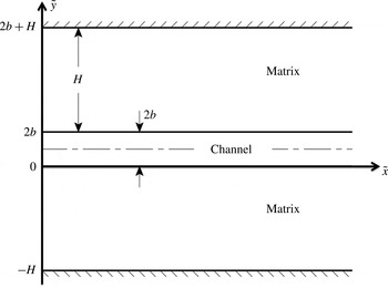
We consider tracer transport in a single-phase fully developed pressure-driven laminar flow in a semi-infinitely long (micro-)channel embedded in a porous matrix with permeability
 $k$
and porosity
 ${\it\phi}$
(figure 1). While the Carman–Kozeny equation establishes a unique relationship between porosity and permeability, it is unable to describe permeability dependences over a broad range of porous medium configurations (Valdes-Parada, Ochoa-Tapia & Alvarez-Ramirez Reference Valdes-Parada, Ochoa-Tapia and Alvarez-Ramirez2009). Without loss of generality, we consider porosity and permeability as independent variables in order to account for the unknown relationship between
 $k$
and the microstructure arrangement. The boundaries between the channel and the matrix walls are located at
 ${\tilde{y}}=0$
and
 ${\tilde{y}}=2b$
. The porous matrix width (thickness) is
 $H$
, i.e. the matrix occupies the domains
 ${\tilde{y}}\in (2b,2b+H)$
and
 ${\tilde{y}}\in (-H,0)$
. A dilute Newtonian solution with density
 ${\it\rho}$
and solute concentration
 $c_{0}$
is injected at the domain inlet
 $\tilde{x}=0$
. Flow and transport occur both in the channel and in the matrix, and are affected by the momentum and mass transfer across the channel–matrix interfaces.
Problem domain.

We denote the concentration and the
 $\tilde{x}$
-component of the velocity in the channel and the matrix by
 $\tilde{c}_{f}$
,
 $\tilde{u} _{f}$
,
 $\tilde{c}_{m}$
and
 $\tilde{u}_{m}$
respectively. Due to the symmetry of the domain, we restrict our analysis to
 ${\tilde{y}}\in (-H,b)$
.
2.1 Flow equations
Fully developed Stokes flow in the channel–matrix system can be described by coupling the Stokes equation in the channel with a Darcy–Brinkman equation in the matrix,
 $$\begin{eqnarray}\displaystyle & \displaystyle {\it\mu}\frac{\text{d}^{2}\tilde{u} _{f}}{\text{d}{\tilde{y}}^{2}}-\frac{\text{d}\tilde{p}}{\text{d}\tilde{x}}=0,\quad {\tilde{y}}\in (0,b), & \displaystyle\end{eqnarray}$$
 $$\begin{eqnarray}\displaystyle & \displaystyle {\it\mu}\frac{\text{d}^{2}\tilde{u}_{m}}{\text{d}{\tilde{y}}^{2}}-\frac{{\it\mu}}{k}\tilde{u}_{m}-\frac{\text{d}\tilde{p}}{\text{d}\tilde{x}}=0,\quad {\tilde{y}}\in (-H,0), & \displaystyle\end{eqnarray}$$
 $\tilde{u} _{i}({\tilde{y}})$
with
 $i=\{f,m\}$
is the
 $\tilde{x}$
-component of the velocity in the channel and the matrix,
 ${\it\mu}$
is the fluid dynamic viscosity,
 $k\,[L^{2}]$
is the matrix permeability, and
 $\text{d}_{\tilde{x}}\tilde{p}$
is a constant pressure gradient driving the flow in the
 $\tilde{x}$
-direction. Equations (2.1) are subject to no-slip and symmetry boundary conditions at the bottom solid wall (
 ${\tilde{y}}=-H$
) and channel centreline (
 ${\tilde{y}}=b$
) respectively, and continuity of velocity and shear stress conditions at the interface separating the channel and the porous matrix (
 ${\tilde{y}}=0$
),
 $$\begin{eqnarray}\left.\tilde{u}_{m}\right|_{{\tilde{y}}=-H}=0,\quad \left.\frac{\text{d}\tilde{u} _{f}}{\text{d}{\tilde{y}}}\right|_{{\tilde{y}}=b}=0,\quad \left.\tilde{u} _{f}\right|_{{\tilde{y}}=0}=\left.\tilde{u}_{m}\right|_{{\tilde{y}}=0},\quad \left.\frac{\text{d}\tilde{u} _{f}}{\text{d}{\tilde{y}}}\right|_{{\tilde{y}}=0}=\left.\frac{\text{d}\tilde{u}_{m}}{\text{d}{\tilde{y}}}\right|_{{\tilde{y}}=0}.\end{eqnarray}$$
While many boundary conditions have been proposed to couple free and filtration flows, see Le Bars & Worster (Reference Le Bars and Worster2006) for a review, continuity of velocity and shear stress has been proven accurate in a number of applications, e.g. Battiato et al. (Reference Battiato, Bandaru and Tartakovsky2010), Battiato (Reference Battiato2012) and Battiato & Rubol (Reference Battiato and Rubol2014).
We define the following dimensionless quantities:
 $$\begin{eqnarray}x=\frac{\tilde{x}}{L},\quad y=\frac{{\tilde{y}}}{b},\quad p=\frac{\tilde{p}}{p_{0}},\quad u_{i}=\frac{\tilde{u} _{i}}{U},\quad \text{with }i=\{f,m\},\end{eqnarray}$$
where
 $L$
is a characteristic macroscopic/observation length scale, e.g. the distance far from the inlet where data are collected,
 $p_{0}$
is a characteristic pressure, e.g. the ambient pressure, and
 $U$
is the average velocity across the channel. Then, (2.1)–(2.2) can be cast in dimensionless form,
 $$\begin{eqnarray}\displaystyle & \displaystyle \frac{\text{d}^{2}u_{f}}{\text{d}y^{2}}-{\it\Psi}=0,\quad y\in (0,1), & \displaystyle\end{eqnarray}$$
 $$\begin{eqnarray}\displaystyle & \displaystyle \frac{\text{d}^{2}u_{m}}{\text{d}y^{2}}-{\it\lambda}^{2}u_{m}-{\it\Psi}=0,\quad y\in (-h,0), & \displaystyle\end{eqnarray}$$
 $$\begin{eqnarray}\left.u_{m}\right|_{y=-h}=0,\quad \left.\frac{\text{d}u_{f}}{\text{d}y}\right|_{y=1}=0,\quad \left.u_{f}\right|_{y=0}=\left.u_{m}\right|_{y=0},\quad \left.\frac{\text{d}u_{f}}{\text{d}y}\right|_{y=0}=\left.\frac{\text{d}u_{m}}{\text{d}y}\right|_{y=0},\end{eqnarray}$$
where
 $$\begin{eqnarray}{\it\lambda}^{2}=\frac{b^{2}}{k},\quad {\it\Psi}=\frac{p_{0}b^{2}}{{\it\mu}UL}\frac{\text{d}p}{\text{d}x}\quad \text{and}\quad h=\frac{H}{b}.\end{eqnarray}$$
The system (2.4) admits an analytical solution for the velocity profiles in the channel and the matrix,
 $u_{f}$
and
 $u_{m}$
respectively,
 $$\begin{eqnarray}\displaystyle & \displaystyle u_{f}(y)=\frac{{\it\Psi}}{2}y^{2}+Ay+B,\quad y\in [0,1], & \displaystyle\end{eqnarray}$$
 $$\begin{eqnarray}\displaystyle & \displaystyle u_{m}(y)=-\frac{{\it\Psi}}{{\it\lambda}^{2}}+E\text{e}^{{\it\lambda}y}+F\text{e}^{-{\it\lambda}y},\quad y\in [-h,0], & \displaystyle\end{eqnarray}$$
where
 $A$
,
 $B$
,
 $E$
and
 $F$
are integration constants,
 $$\begin{eqnarray}\displaystyle A & = & \displaystyle -{\it\Psi},\end{eqnarray}$$
 $$\begin{eqnarray}\displaystyle B & = & \displaystyle -\frac{{\it\Psi}}{{\it\lambda}^{2}}(-1+\text{e}^{{\it\Lambda}})(-1+\text{e}^{{\it\Lambda}}+{\it\lambda}+{\it\lambda}\text{e}^{{\it\Lambda}})(1+\text{e}^{2{\it\Lambda}})^{-1},\end{eqnarray}$$
 $$\begin{eqnarray}\displaystyle E & = & \displaystyle -\frac{{\it\Psi}}{{\it\lambda}^{2}}\text{e}^{{\it\Lambda}}(-1+{\it\lambda}\text{e}^{{\it\Lambda}})(1+\text{e}^{2{\it\Lambda}})^{-1},\end{eqnarray}$$
 $$\begin{eqnarray}\displaystyle F & = & \displaystyle -\frac{{\it\Psi}}{{\it\lambda}^{2}}({\it\lambda}+\text{e}^{{\it\Lambda}})(1+\text{e}^{2{\it\Lambda}})^{-1}.\end{eqnarray}$$
 $$\begin{eqnarray}{\it\Lambda}={\it\lambda}h,\end{eqnarray}$$
which represents a characteristic dimensionless length scale, also known as the penetration length, associated with the thickness of the boundary layer between the free and filtration flows (Nepf Reference Nepf2012). A classification between thin (
 ${\it\Lambda}\ll 1$
) and thick porous media (
 ${\it\Lambda}\gg 1$
) can be introduced based on the magnitude of
 ${\it\Lambda}$
(Battiato Reference Battiato2012). The slip velocity,
 $U_{slip}$
, can be readily calculated as
 $U_{slip}:=u_{m}(y=0)=u_{f}(y=0)$
, i.e.
 $$\begin{eqnarray}U_{slip}=-{\it\Psi}\frac{h(\text{e}^{{\it\Lambda}}-1)[{\it\Lambda}(\text{e}^{{\it\Lambda}}+1)+h(\text{e}^{{\it\Lambda}}-1)]}{{\it\Lambda}^{2}(1+\text{e}^{2{\it\Lambda}})}.\end{eqnarray}$$
2.2 Transport equations
We consider transport of a passive scalar injected at the channel inlet, i.e.
 $\tilde{x}=0$
and
 ${\tilde{y}}\in (0,b)$
, with concentration
 $c_{0}$
for
 $\tilde{t}>0$
. The solute concentrations in the channel
 $\tilde{c}_{f}$
and the matrix
 $\tilde{c}_{m}$
satisfy a system of coupled advection–dispersion equations,
 $$\begin{eqnarray}\displaystyle \frac{\partial \tilde{c}_{f}}{\partial \tilde{t}}+\tilde{u} _{f}\frac{\partial \tilde{c}_{f}}{\partial \tilde{x}} & = & \displaystyle \tilde{D}_{f}\left(\frac{\partial ^{2}\tilde{c}_{f}}{\partial \tilde{x}^{2}}+\frac{\partial ^{2}\tilde{c}_{f}}{\partial {\tilde{y}}^{2}}\right),\quad {\tilde{y}}\in (0,b),\quad \tilde{x},\tilde{t}>0,\end{eqnarray}$$
 $$\begin{eqnarray}\displaystyle \frac{\partial \tilde{c}_{m}}{\partial \tilde{t}}+\tilde{u}_{m}\frac{\partial \tilde{c}_{m}}{\partial \tilde{x}} & = & \displaystyle \tilde{D}_{mx}\frac{\partial ^{2}\tilde{c}_{m}}{\partial \tilde{x}^{2}}+\tilde{D}_{my}\frac{\partial ^{2}\tilde{c}_{m}}{\partial {\tilde{y}}^{2}},\quad {\tilde{y}}\in (-H,0),\quad \tilde{x},\tilde{t}>0,\end{eqnarray}$$
 $\tilde{D}_{f}$
is the molecular diffusion coefficient,
 $\tilde{D}_{mx}$
and
 $\tilde{D}_{my}$
are the
 $\tilde{x}$
and
 ${\tilde{y}}$
components of the dispersion coefficient in the matrix, and
 $\tilde{u} _{f}=Uu_{f}$
and
 $\tilde{u}_{m}=Uu_{m}$
are defined by (2.7) and (2.8) respectively. Equations (2.12) are subject to initial,
 $$\begin{eqnarray}\tilde{c}_{f}(\tilde{x},{\tilde{y}},\tilde{t}=0)=0\quad \text{and}\quad \tilde{c}_{m}(\tilde{x},{\tilde{y}},\tilde{t}=0)=0,\end{eqnarray}$$
and boundary conditions,
 $$\begin{eqnarray}\tilde{c}_{f}(0,{\tilde{y}}\in [0,b],\tilde{t})=c_{0},\quad \tilde{c}_{f}(\infty ,{\tilde{y}}\in [0,b],\tilde{t})=0,\quad \frac{\partial \tilde{c}_{f}}{\partial {\tilde{y}}}(\tilde{x},b,\tilde{t})=0,\end{eqnarray}$$
 $$\begin{eqnarray}\frac{\partial \tilde{c}_{m}}{\partial \tilde{x}}(0,{\tilde{y}}\in [-H,0),\tilde{t})=0,\quad \tilde{c}_{m}(\infty ,{\tilde{y}}\in [-H,0],\tilde{t})=0,\quad \frac{\partial \tilde{c}_{m}}{\partial {\tilde{y}}}(\tilde{x},-H,\tilde{t})=0.\end{eqnarray}$$
Additionally, on the channel–matrix interface, the continuity of concentration and mass flux is satisfied,
 $$\begin{eqnarray}\tilde{c}_{f}(\tilde{x},0,\tilde{t})=\tilde{c}_{m}(\tilde{x},0,\tilde{t})\quad \text{and}\quad \frac{\partial \tilde{c}_{f}}{\partial {\tilde{y}}}(\tilde{x},0,\tilde{t})=\frac{{\it\phi}\tilde{D}_{my}}{\tilde{D}_{f}}\frac{\partial \tilde{c}_{m}}{\partial {\tilde{y}}}(\tilde{x},0,\tilde{t}),\end{eqnarray}$$
where
 ${\it\phi}$
is the matrix porosity. We define the following dimensionless quantities:
 $$\begin{eqnarray}t=\frac{U}{L}\tilde{t},\quad D_{f}=\frac{\tilde{D}_{f}}{D^{\star }},\quad D_{mi}=\frac{\tilde{D}_{mi}}{D^{\star }},\quad c_{i}=\frac{\tilde{c}_{i}}{c_{0}},\quad \text{with }i=\{\hspace{1.5pt}f,m\}.\end{eqnarray}$$
Here,
 $D^{\star }=O(\tilde{D}_{f})$
is the order of magnitude of the solute molecular diffusion coefficient, such that
 $D_{f}=O(1)$
. Since we investigate the dynamics of transport in a time frame much larger than the diffusion time,
 ${\it\tau}_{d}=b^{2}/D^{\star }$
, and close to the advection time,
 ${\it\tau}_{a}=L/U$
, all of the time scales are scaled by
 ${\it\tau}_{a}$
. Then, (2.12) can be written in dimensionless form as follows:
 $$\begin{eqnarray}\displaystyle {\it\epsilon}Pe\frac{\partial c_{f}}{\partial t}+{\it\epsilon}Peu_{f}\frac{\partial c_{f}}{\partial x} & = & \displaystyle {\it\epsilon}^{2}D_{f}\frac{\partial ^{2}c_{f}}{\partial x^{2}}+D_{f}\frac{\partial ^{2}c_{f}}{\partial y^{2}},\quad y\in (0,1),\quad x,t>0,\quad\end{eqnarray}$$
 $$\begin{eqnarray}\displaystyle {\it\epsilon}Pe\frac{\partial c_{m}}{\partial t}+{\it\epsilon}Peu_{m}\frac{\partial c_{m}}{\partial x} & = & \displaystyle {\it\epsilon}^{2}D_{mx}\frac{\partial ^{2}c_{m}}{\partial x^{2}}+D_{my}\frac{\partial ^{2}c_{m}}{\partial y^{2}},\quad y\in (-h,0),\quad x,t>0,\quad\end{eqnarray}$$
 $$\begin{eqnarray}{\it\epsilon}=\frac{b}{L}\quad \text{and}\quad Pe=\frac{{\it\tau}_{d}}{{\it\tau}_{a}}=\frac{Ub}{D^{\star }}.\end{eqnarray}$$
Equations (2.18) are subject to
 $$\begin{eqnarray}c_{f}(0,y\in [0,1],t)=1,\quad c_{f}(\infty ,y\in [0,1],t)=0,\quad \frac{\partial c_{f}}{\partial y}(x,1,t)=0,\end{eqnarray}$$
 $$\begin{eqnarray}\frac{\partial c_{m}}{\partial x}(0,y\in [-h,0),t)=0,\quad c_{m}(\infty ,y\in [-h,0],t)=0,\quad \frac{\partial c_{m}}{\partial y}(x,-h,t)=0,\end{eqnarray}$$
 $$\begin{eqnarray}c_{f}(x,0,t)=c_{m}(x,0,t)\quad \text{and}\quad \frac{\partial c_{f}}{\partial y}(x,0,t)=\frac{{\it\phi}D_{my}}{D_{f}}\frac{\partial c_{m}}{\partial y}(x,0,t).\end{eqnarray}$$
In the following section, we employ asymptotic homogenization to relate the dispersion coefficient in the coupled channel–matrix system with the effective properties of the matrix.
3 Asymptotic homogenization and upscaled equations
To derive the upscaled transport equations, we apply rescaling and asymptotic analysis to the ADEs (2.18). We introduce the rescaled longitudinal coordinate
 ${\it\xi}$
and a coefficient
 ${\it\alpha}$
such that
 $$\begin{eqnarray}x:={\it\xi}\sqrt{{\it\epsilon}}\quad \text{and}\quad Pe:={\it\epsilon}^{-{\it\alpha}}.\end{eqnarray}$$
Equations (2.18a ) and (2.18b ) take the form
 $$\begin{eqnarray}\displaystyle {\it\epsilon}Pe\left(\frac{\partial c_{f}}{\partial t}+\frac{u_{f}}{\sqrt{{\it\epsilon}}}\frac{\partial c_{f}}{\partial {\it\xi}}\right) & = & \displaystyle {\it\epsilon}D_{f}\frac{\partial ^{2}c_{f}}{\partial {\it\xi}^{2}}+D_{f}\frac{\partial ^{2}c_{f}}{\partial y^{2}},\end{eqnarray}$$
 $$\begin{eqnarray}\displaystyle {\it\epsilon}Pe\left(\frac{\partial c_{m}}{\partial t}+\frac{u_{m}}{\sqrt{{\it\epsilon}}}\frac{\partial c_{m}}{\partial {\it\xi}}\right) & = & \displaystyle {\it\epsilon}D_{mx}\frac{\partial ^{2}c_{m}}{\partial {\it\xi}^{2}}+D_{my}\frac{\partial ^{2}c_{m}}{\partial y^{2}}.\end{eqnarray}$$
 $$\begin{eqnarray}\langle \cdot \rangle =\frac{1}{L^{\star }}\int _{0}^{L^{\star }}\,\text{d}y,\end{eqnarray}$$
where
 $L^{\star }=1$
for the channel and
 $L^{\star }=-h$
for the matrix. Moreover, we employ the ansatz
 $$\begin{eqnarray}c_{i}=c_{i}^{(0)}({\it\xi},t)+\sqrt{{\it\epsilon}}c_{i}^{(1)}({\it\xi},y,t)+{\it\epsilon}c_{i}^{(2)}({\it\xi},y,t)+O({\it\epsilon}\sqrt{{\it\epsilon}}),\quad i=\{f,m\},\end{eqnarray}$$
where
 $c_{i}^{(j)}$
is the
 $j$
th-order term in the expansion of concentration
 $c_{i}$
. Substituting (3.4) in (3.2) while applying the averaging operator (3.3) leads to a system of coupled upscaled (effective macroscopic) equations (see Appendix)
 $$\begin{eqnarray}\displaystyle {\it\epsilon}^{2}Pe\left(\frac{\partial \langle c_{f}\rangle }{\partial t}+\langle u_{f}\rangle \frac{\partial \langle c_{f}\rangle }{\partial x}\right) & = & \displaystyle {\it\epsilon}^{3}D_{f}^{\star }\frac{\partial ^{2}\langle c_{f}\rangle }{\partial x^{2}}-{\it\phi}\left[{\it\epsilon}^{2}PeN_{1}\frac{\partial \langle c_{m}\rangle }{\partial x}+\frac{3D_{my}}{h}(\langle c_{f}\rangle -\langle c_{m}\rangle )\right],\nonumber\\ \displaystyle & & \displaystyle\end{eqnarray}$$
 $$\begin{eqnarray}\displaystyle {\it\epsilon}^{2}Pe\left(\frac{\partial \langle c_{m}\rangle }{\partial t}+\langle u_{m}\rangle \frac{\partial \langle c_{m}\rangle }{\partial x}\right) & = & \displaystyle {\it\epsilon}^{3}D_{m}^{\star }\frac{\partial ^{2}\langle c_{m}\rangle }{\partial x^{2}}+\frac{1}{{\it\phi}}\left[{\it\epsilon}^{2}Pe\frac{M_{1}}{h}\frac{\partial \langle c_{f}\rangle }{\partial x}+\frac{3D_{f}}{h}(\langle c_{f}\rangle -\langle c_{m}\rangle )\right],\nonumber\\ \displaystyle & & \displaystyle\end{eqnarray}$$
 $$\begin{eqnarray}M_{1}=-\!\left(\frac{{\it\Psi}}{6}+\frac{A}{2}+B\right)\quad \text{and}\quad N_{1}=\frac{{\it\Psi}h}{{\it\lambda}^{2}}-\frac{F}{{\it\lambda}}(\text{e}^{{\it\lambda}h}-1)+\frac{E}{{\it\lambda}}(\text{e}^{-{\it\Lambda}}-1),\end{eqnarray}$$
subject to
 $$\begin{eqnarray}\langle c_{f}\rangle (x=0,t)=1,\quad \langle c_{f}\rangle (x=\infty ,t)=0,\quad \langle c_{f}\rangle (x,t=0)=0,\end{eqnarray}$$
 $$\begin{eqnarray}\frac{\partial \langle c_{m}\rangle }{\partial x}(x=0,t)=0,\quad \langle c_{m}\rangle (x=\infty ,t)=0,\quad \langle c_{m}\rangle (x,t=0)=0,\end{eqnarray}$$
under the assumption that
 $\langle c_{i}^{(1)}\rangle =\langle c_{i}^{(2)}\rangle =0$
,
 $i=\{\,f,m\}$
, and provided that the conditions
-
(1)
 ${\it\epsilon}\ll 1$
,
-
(2)
$Pe<{\it\epsilon}^{-1/2}$


are met. Condition (1) ensures that geometric scale separation exists and is satisfied when the channel is long and thin. Condition (2) provides an upper bound on the Péclet number. To ensure that the higher-order correction terms have zero mean, we set
 $\langle c_{i}^{(1)}\rangle =\langle c_{i}^{(2)}\rangle =0$
(Mikelic et al.
Reference Mikelic, Devigne and Duijn2006).
The advection–dispersion equations (3.5) are coupled through a source term describing the mass exchange between the matrix and the channel. Unlike existing works (Reichert & Wanner Reference Reichert and Wanner1991; Kazezyılmaz-Alhan Reference Kazezyılmaz-Alhan2008), which have postulated the coupling in the form of a storage term only, i.e.
 $(\langle c_{f}\rangle -\langle c_{m}\rangle )$
, our analysis demonstrates that an additional contribution due to concentration gradients along the channel, i.e.
 $\partial \langle c_{i}\rangle /\partial x$
,
 $i=\{m,f\}$
, must be considered as well. We emphasize that the flux
 $\partial \langle c_{m}\rangle /\partial x$
is an advective term contributed by the non-zero permeability matrix. This is different from Tang et al. (Reference Tang, Frind and Sudicky1981), Dejam et al. (Reference Dejam, Hassanzadeh and Chen2014) or Roubinet et al. (Reference Roubinet, Dreuzy and Tartakovsky2012), who only consider diffusive transport in the porous medium.
In (3.5),
 $D_{f}^{\star }$
and
 $D_{m}^{\star }$
are the dispersion coefficients for the channel and the matrix respectively. The channel dispersion coefficient
 $D_{f}^{\star }$
is defined as
 $$\begin{eqnarray}D_{f}^{\star }=D_{f}+Pe^{2}\frac{I_{f}}{D_{f}},\end{eqnarray}$$
or, equivalently and without loss of generality,
 $$\begin{eqnarray}D_{f}^{\star }=1+Pe^{2}I_{f},\end{eqnarray}$$
if
 $D^{\star }\equiv \tilde{D}_{f}$
and
 $D_{f}\equiv 1$
in (3.2) and (3.9) respectively. In the following, we will use the second expression (3.10) (i.e.
 $D_{f}\equiv 1$
), as it allows a direct comparison with formulae derived by other authors (Horne & Rodriguez Reference Horne and Rodriguez1983; Griffiths et al.
Reference Griffiths, Howell and Shipley2013; Dejam et al.
Reference Dejam, Hassanzadeh and Chen2014). In (3.10),
 $I_{f}=(3/560){\it\Psi}^{2}+(1/40)A{\it\Psi}+(7/360)B{\it\Psi}+(7/240)A^{2}+(1/24)AB$
, i.e.
 $$\begin{eqnarray}I_{f}=\frac{{\it\Psi}^{2}}{105}[1+g({\it\lambda},{\it\Lambda})],\end{eqnarray}$$
where
 $$\begin{eqnarray}g({\it\lambda},{\it\Lambda})=\frac{7}{3}\frac{(\text{e}^{{\it\Lambda}}-1)[\text{e}^{{\it\Lambda}}-1+{\it\lambda}(1+\text{e}^{{\it\Lambda}})]}{{\it\lambda}^{2}(1+\text{e}^{2{\it\Lambda}})},\end{eqnarray}$$
or, equivalently,
 $$\begin{eqnarray}g({\it\lambda},{\it\Lambda})=\frac{7}{3{\it\lambda}}\left[\text{tanh}{\it\Lambda}+\frac{1}{{\it\lambda}}\left(1-\text{sech}{\it\Lambda}\right)\right].\end{eqnarray}$$
Moreover, from (2.11) it is immediate to show that
 $$\begin{eqnarray}\frac{U_{slip}}{{\it\Psi}}=-\frac{3}{7}g({\it\lambda},{\it\Lambda}),\end{eqnarray}$$
i.e. the normalized interfacial velocity
 $-U_{slip}/{\it\Psi}$
is solely controlled by the porous matrix properties.
We emphasize that
 $D_{f}^{\star }$
explicitly depends on
 ${\it\lambda}$
(inverse of the dimensionless permeability) through
 $I_{f}$
. The matrix dispersion coefficient is
 $$\begin{eqnarray}D_{m}^{\star }=D_{mx}-Pe^{2}\frac{I_{m}}{D_{my}},\end{eqnarray}$$
where
 $$\begin{eqnarray}I_{m}=\frac{1}{h}\int _{-h}^{0}u_{m}(y)N(y)\,\text{d}y\end{eqnarray}$$
and
 $$\begin{eqnarray}N(y)=\int _{0}^{y}\,\text{d}y^{\prime }\int _{0}^{y^{\prime }}u_{m}(y^{\star })\,\text{d}y^{\star },\quad 0<y^{\star }<y^{\prime },\;0<y^{\prime }<y.\end{eqnarray}$$
The derivation details are presented in the Appendix.
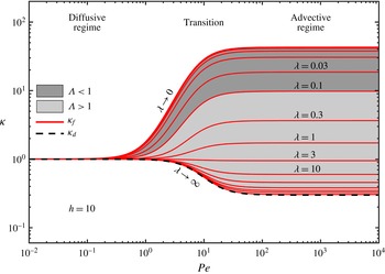
Normalized dispersion coefficients
 ${\it\kappa}_{f}$
(solid red lines) and
 ${\it\kappa}_{d}$
(dashed back line) versus
 $Pe$
for different values of
 ${\it\lambda}$
and
 ${\it\Lambda}$
. Here,
 ${\it\Psi}=-0.78$
and
 $h=10$
.

4 Dispersion coefficient and matrix properties
In order to investigate the impact of the matrix effective properties,
 $h$
and
 ${\it\lambda}$
, on macroscale transport in the channel, we compare
 $D_{f}^{\star }$
in (3.10) with the dispersion coefficient
 $D_{d}$
obtained by Dejam et al. (Reference Dejam, Hassanzadeh and Chen2014) for a coupled system with purely diffusive transport in the matrix (i.e.
 ${\it\lambda}\rightarrow \infty$
or
 $k\rightarrow 0$
, and
 $h\neq 0$
). To isolate the effect of the width of the porous medium and its permeability,
 $h$
and
 ${\it\lambda}$
, on channel macroscopic transport, we normalize both coefficients by the Aris–Taylor dispersion coefficient
 $D_{AT}$
for a single channel (i.e.
 ${\it\lambda}\rightarrow \infty$
or
 $k\rightarrow 0$
, and
 $h=0$
) and define
 $$\begin{eqnarray}{\it\kappa}_{f}:=\frac{D_{f}^{\star }}{D_{AT}}\quad \text{and}\quad {\it\kappa}_{d}:=\frac{D_{d}}{D_{AT}},\end{eqnarray}$$
where (Horne & Rodriguez Reference Horne and Rodriguez1983; Dejam et al. Reference Dejam, Hassanzadeh and Chen2014)
 $$\begin{eqnarray}D_{d}=1+\frac{1}{175}Pe^{2}\quad \text{and}\quad D_{AT}=1+\frac{2}{105}Pe^{2}.\end{eqnarray}$$
In figure 2, we plot
 ${\it\kappa}_{f}$
and
 ${\it\kappa}_{d}$
as a function of
 $Pe$
and
 ${\it\lambda}$
, for a fixed
 $h$
. The figure shows that two thresholds exist, such that
 ${\it\kappa}_{f}$
is constant for
 $Pe<Pe_{min}$
and
 $Pe>Pe^{\star }$
. For small Péclet number (
 $Pe<Pe_{min}\approx 1$
),
 ${\it\kappa}_{f}\rightarrow {\it\kappa}_{d}$
, i.e. the dispersion coefficient for the coupled system with permeable matrix (finite
 ${\it\lambda}$
) converges to its non-permeable matrix limit (
 ${\it\lambda}\rightarrow \infty$
,
 $h\neq 0$
) independent of
 $h$
and
 ${\it\lambda}$
. When
 $Pe<1$
, advective mixing both in the matrix and in the channel is negligible relative to diffusive mixing. As a result,
 ${\it\kappa}_{f}\rightarrow {\it\kappa}_{d}$
and
 ${\it\kappa}_{d}\rightarrow 1$
. In the intermediate range of Péclet numbers (
 $1<Pe<Pe^{\star }$
),
 ${\it\kappa}_{f}$
changes from
 ${\it\kappa}_{f}=1$
to
 ${\it\kappa}_{f}={\it\kappa}_{f}({\it\lambda},h)$
when
 $Pe>Pe^{\star }$
. It is worth noticing that the dispersion coefficient can overcome its purely diffusive limit when
 ${\it\lambda}<1$
, i.e. mixing is enhanced compared with a channel of half-width
 $b$
. When
 $1<Pe<Pe^{\star }$
,
 ${\it\kappa}_{f}$
is a function of
 $Pe$
,
 $h$
and
 ${\it\lambda}$
. Therefore, the matrix properties (or
 ${\it\lambda}$
and
 $h$
) and boundary conditions (or
 $Pe$
) can be independently modified to achieve the desired dispersion coefficient.
As mentioned above, for large Péclet number (
 $Pe>Pe^{\star }$
),
 ${\it\kappa}_{f}$
reaches a
 $Pe$
-independent asymptotic value
 ${\it\kappa}_{{\it\lambda},h}$
, i.e.
 $\lim _{Pe\rightarrow \infty }{\it\kappa}_{f}={\it\kappa}_{{\it\lambda},h}$
. In this regime, for any given
 $Pe$
, the dispersion coefficient increases with decreasing
 ${\it\lambda}$
(figure 2). This phenomenon is attributed to a decreasing mass flux at the interface between the channel and the matrix, and a resulting decreasing mass loss towards the matrix. Such mass loss is smaller compared with the zero-permeability case, where no solute is transported from the upper steam by the flow in the matrix. This is a newly identified mechanism regulating mass exchange between the channel and the matrix, which is purely controlled by the matrix properties (
 ${\it\lambda}$
and
 $h$
) at fixed operating conditions (i.e. constant Péclet number). This mechanism is different from the mass transfer mechanism first proposed by Wu, Ye & Sudicky (Reference Wu, Ye and Sudicky2010) and then quantified by Dejam et al. (Reference Dejam, Hassanzadeh and Chen2014), where the channel–matrix interface flux increases (and the dimensionless dispersion coefficient
 ${\it\kappa}_{d}$
decreases) with increasing Péclet number and is independent of the matrix properties
 ${\it\lambda}$
and
 $h$
. In the zero-permeability limit, i.e.
 ${\it\lambda}\rightarrow \infty$
, and for fixed
 $Pe$
,
 ${\it\kappa}_{f}\rightarrow {\it\kappa}_{d}$
, as expected. In the following, we focus on the study of the dispersion coefficient in the matrix,
 ${\it\kappa}_{f}$
, only, since it is deemed more relevant to many engineering applications where transverse mixing enhancement in the channel is the primary target.
We aim to identify the scaling behaviour of
 ${\it\kappa}_{f}$
in different regimes, if it exists. Combining (3.11) and (3.10) with (4.1) leads to
 $$\begin{eqnarray}{\it\kappa}_{f}=105\frac{1+Pe^{2}I_{f}}{105+2Pe^{2}},\end{eqnarray}$$
with
 $I_{f}$
given by (3.11). We define
 ${\it\kappa}_{f,Pe\rightarrow 0}$
and
 ${\it\kappa}_{f,{\it\lambda}\rightarrow \infty }$
as the fracture dimensionless dispersion coefficients in the two purely diffusive limits:
 $Pe\rightarrow 0$
for any
 ${\it\lambda}$
, and
 ${\it\lambda}\rightarrow \infty$
for any
 $Pe$
respectively. The coefficient
 ${\it\kappa}_{f,Pe\rightarrow 0}$
corresponds to the scenario where mass transport in the matrix is driven solely by diffusion since
 $Pe=0$
;
 ${\it\kappa}_{f,{\it\lambda}\rightarrow \infty }$
corresponds to the case of diffusive transport in an impermeable matrix. The latter differs from Aris–Taylor dispersion in that the channel–porous interface is impermeable to flow, but permeable to mass. If
 $Pe\rightarrow 0$
,
 $D_{f}^{\star }=1$
and
 $$\begin{eqnarray}{\it\kappa}_{f,Pe\rightarrow 0}:=\frac{\lim _{Pe\rightarrow 0}D_{f}^{\star }}{D_{AT}}=\frac{105}{105+2Pe^{2}}.\end{eqnarray}$$
Since
 ${\it\Lambda}\rightarrow \infty$
when
 ${\it\lambda}\rightarrow \infty$
for
 $h\neq 0$
, then
 $$\begin{eqnarray}{\it\kappa}_{f,{\it\lambda}\rightarrow \infty }:=\frac{\lim _{{\it\lambda}\rightarrow \infty }D_{f}^{\star }}{D_{AT}}=\frac{105+Pe^{2}{\it\Psi}^{2}}{105+2Pe^{2}}.\end{eqnarray}$$
Combining (4.4) and (4.5) with (4.3) leads to the following expression for
 ${\it\kappa}_{f}$
:
 $$\begin{eqnarray}{\it\kappa}_{f}={\it\kappa}_{f,Pe\rightarrow 0}+g({\it\Lambda},{\it\lambda})\cdot ({\it\kappa}_{f,{\it\lambda}\rightarrow \infty }-{\it\kappa}_{f,Pe\rightarrow 0}),\end{eqnarray}$$
where
 $g({\it\Lambda},h)$
is defined in (3.13). In order to isolate the dependence of
 ${\it\kappa}_{f}$
from the matrix properties,
 ${\it\lambda}$
and
 $h$
, we define the normalized dimensionless dispersion coefficient
 ${\it\Pi}$
,
 $$\begin{eqnarray}{\it\Pi}:=\frac{{\it\kappa}_{f}-{\it\kappa}_{f,Pe\rightarrow 0}}{{\it\kappa}_{f,{\it\lambda}\rightarrow \infty }-{\it\kappa}_{f,Pe\rightarrow 0}},\end{eqnarray}$$
which satisfies
 $$\begin{eqnarray}{\it\Pi}=g({\it\Lambda},{\it\lambda})=-\frac{7}{3}\frac{U_{slip}}{{\it\Psi}},\end{eqnarray}$$
i.e. it is independent of
 $Pe$
. It is worth noticing that
 ${\it\Pi}$
scales as
 $U_{slip}$
normalized by
 ${\it\Psi}$
. In figure 2,
 ${\it\kappa}_{f}$
reaches a
 $Pe$
-independent threshold when
 $Pe\rightarrow \infty$
. Since
 $\lim _{Pe\rightarrow \infty }({\it\kappa}_{f,Pe\rightarrow 0})=0$
and
 $\lim _{Pe\rightarrow \infty }({\it\kappa}_{f,{\it\lambda}\rightarrow \infty })={\it\Psi}^{2}/2$
, then
 $$\begin{eqnarray}\lim _{Pe\rightarrow \infty }{\it\kappa}_{f}\sim \lim _{Pe\rightarrow \infty }{\it\Pi}.\end{eqnarray}$$
From (4.8), we obtain
 $$\begin{eqnarray}{\it\kappa}_{f}^{threshold}=\lim _{Pe\rightarrow \infty }{\it\kappa}_{f}=-\frac{7{\it\Psi}}{6}U_{slip}={\displaystyle \frac{{\it\Psi}^{2}}{2}}{\it\Pi},\end{eqnarray}$$
i.e. in the advective limit the dispersion coefficient is controlled by the slip velocity at the interface between the porous matrix and the channel.
In the following, we study the scaling behaviour of
 ${\it\Pi}$
(or
 $U_{slip}/{\it\Psi}$
) for thin (
 ${\it\Lambda}\ll 1$
) and thick (
 ${\it\Lambda}\gg 1$
) porous matrices.
4.1 Thin porous matrix limit,
${\it\Lambda}\ll 1$

The asymptotic expansion of (4.8) about
 ${\it\Lambda}=0$
leads to
 $$\begin{eqnarray}{\it\Pi}=\frac{7}{3}\left[\left(h+\frac{h^{2}}{2}\right)-\left(\frac{h}{3}+\frac{5h^{2}}{24}\right){\it\Lambda}^{2}+O({\it\Lambda}^{5})\right],\end{eqnarray}$$
since
 $\text{tanh}{\it\Lambda}\approx {\it\Lambda}-{\it\Lambda}^{3}/3+O({\it\Lambda}^{5})$
and
 $\text{sech}{\it\Lambda}\approx 1-{\it\Lambda}^{2}/2+5{\it\Lambda}^{4}/24+O({\it\Lambda}^{6})$
. Retaining the leading-order term, we obtain
 $$\begin{eqnarray}{\it\Pi}\sim h\left(1+\frac{h}{2}\right),\quad \text{for }{\it\Lambda}\ll 1,\end{eqnarray}$$
which shows that the dispersion is controlled by the matrix thickness
 $h$
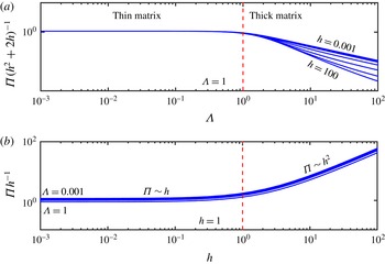
for thin porous layers. Figure 3(a) shows the scaling behaviour of
 ${\it\Pi}(h^{2}+2h)^{-1}$
versus
 ${\it\Lambda}$
and suggests that the scaling (4.12) is a valid approximation for
 ${\it\Lambda}\rightarrow 1$
as well, i.e.
 $$\begin{eqnarray}{\it\Pi}\sim h\left(1+\frac{h}{2}\right),\quad \text{for }{\it\Lambda}\lesssim 1.\end{eqnarray}$$
Further, two scaling regimes exist for
 $h\ll 1$
and
 $h\gg 1$
, i.e.
 $$\begin{eqnarray}\displaystyle {\it\Pi} & {\sim} & \displaystyle h,\quad \text{for }{\it\Lambda}\lesssim 1,\;h\ll 1\end{eqnarray}$$
 $$\begin{eqnarray}\displaystyle {\it\Pi} & {\sim} & \displaystyle h^{2},\quad \text{for }{\it\Lambda}\lesssim 1,\;h\gg 1.\end{eqnarray}$$
 ${\it\Pi}h^{-1}$
as a function of
 $h$
for different
 ${\it\Lambda}\in [0.001,1]$
. As expected,
 ${\it\Pi}h^{-1}$
is constant when
 $h\ll 1$
and grows linearly with
 $h$
when
 $h\gg 1$
. This result suggests that transverse mixing in a channel with a thin porous coating (
 ${\it\Lambda}\ll 1$
) is controlled by
 $h$
, and is more sensitive to the matrix width when
 $h\gg 1$
, i.e. for a given increase in
 $H$
,
 ${\rm\Delta}H$
, better mixing can be achieved if
 $H>b$
.
4.2 Thick porous matrix limit,
${\it\Lambda}\gg 1$

In the limit
 ${\it\Lambda}\gg 1$
, i.e. for thick porous matrices, we expand (4.8) about
 $1/{\it\Lambda}=0$
and obtain
 $$\begin{eqnarray}{\it\Pi}=\frac{7}{3}\frac{(h{\it\Lambda}^{-1}+h^{2}{\it\Lambda}^{-2})\text{e}^{2{\it\Lambda}}-h^{2}{\it\Lambda}^{-2}\text{e}^{{\it\Lambda}}-h{\it\Lambda}^{-1}}{1+\text{e}^{2{\it\Lambda}}}+O({\it\Lambda}^{-2}),\end{eqnarray}$$
since
 $\text{e}^{{\it\Lambda}}(1+\text{e}^{2{\it\Lambda}})^{-1}\rightarrow 0$
and
 $\text{e}^{2{\it\Lambda}}(1+\text{e}^{2{\it\Lambda}})^{-1}\rightarrow 1$
when
 ${\it\Lambda}\rightarrow \infty$
. At the leading order,
 $$\begin{eqnarray}{\it\Pi}\sim \frac{1}{{\it\lambda}},\quad \text{for }{\it\Lambda}\gg 1,\end{eqnarray}$$
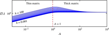
i.e. the normalized dispersion is controlled by the matrix permeability only. Figure 4 shows that
 ${\it\Pi}{\it\lambda}$
reaches a
 ${\it\Lambda}$
-independent value for
 ${\it\Lambda}\gg 1$
, as suggested by (4.16). This analysis shows that when increasing the thickness of the matrix for a given
 ${\it\lambda}$
, further increments of
 $h$
will no longer affect the slip velocity when
 ${\it\Lambda}\gg 1$
. In this regime, the bottom wall of the matrix (located at
 $y=-h$
) becomes ‘invisible’ to the flow and transport in the channel, and changes in
 $h$
will not influence the channel dynamics. For a given channel–matrix system with
 ${\it\Lambda}\gg 1$
, an effective control of the dispersion can be achieved by modifying the permeability of the porous medium.
(a) Scaling behaviour of the normalized dispersion coefficient
 ${\it\Pi}$
defined in (4.7) for thin porous media (
 ${\it\Lambda}\lesssim 1$
) and (b)
 $h<1$
and
 $h>1$
. The coefficient
 ${\it\Pi}$
, i.e. transverse dispersion, is controlled by the width
 $h$
of the porous matrix when
 ${\it\Lambda}\lesssim 1$
; this dependence goes from linear to quadratic as
 $h$
increases above the threshold
 $h\approx 1$
.

Scaling behaviour of the normalized dispersion coefficient
 ${\it\Pi}$
defined in (4.7) for thick porous media (
 ${\it\Lambda}\gg 1$
). The normalized dispersion coefficient is controlled by the matrix permeability only when
 ${\it\Lambda}\gg 1$
.

5 Validation and model accuracy: numerical experiments
The system (3.5) is composed of two one-dimensional transient coupled upscaled equations. The coupling is due to the mass exchange at the interface between the channel and the matrix. Here, we solve the coupled system (3.5) numerically. We test the accuracy of the upscaling approximation (3.5a ) and (3.5b ) by comparison with the averaged 2D solution obtained from numerically solving (2.18a ) and (2.18b ).
5.1 Code validation
For the discretization of the 1D equations (3.5), we use implicit Euler in time and second-order central finite difference discretization in space. For the 2D equations (2.18), we use backward Euler for the time discretization and second-order discretization in space, with upwinding for the advective term and central finite differences for the other terms. A convergence study is performed on the 1D solver by refining the grid size and time step. We validate the 2D solver by setting
 ${\it\phi}=1$
,
 $D_{f}=D_{mx}=D_{my}$
and
 $u_{f}=u_{m}=u^{\star }$
in (2.18). This corresponds to passive transport in a single channel (and no porous medium) with uniform velocity
 $u^{\star }$
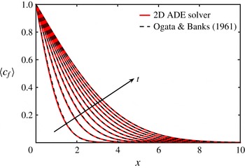
for which a closed-form analytical solution is available (Ogata & Banks Reference Ogata and Banks1961). We compare the numerical average of the pore-scale concentration
 $c_{f}$
with the analytical solution for the continuous injection of a passive solute. The mean concentration profile satisfies (Ogata & Banks Reference Ogata and Banks1961)
 $$\begin{eqnarray}\langle c_{f}\rangle (x,t)=\frac{1}{2}\left[\text{erfc}\left(\frac{x-u^{\star }t}{2\sqrt{D_{f}t}}\right)+\text{exp}\left(\frac{u^{\star }x}{D_{f}}\right)\text{erfc}\left(\frac{x+u^{\star }t}{2\sqrt{D_{f}t}}\right)\right].\end{eqnarray}$$
Comparison between the averaged 2D concentration in the channel and the 1D analytical solution, equation (5.1) (Ogata & Banks Reference Ogata and Banks1961), for passive scalar transport in a single channel with uniform velocity and constant injection. The average concentration
 $\langle c_{f}\rangle$
is plotted in terms of the dimensionless distance from the channel inlet at different instances in time
 $\tilde{t}$
. Here,
 $h=10$
,
 ${\it\phi}=1$
,
 ${\it\epsilon}=0.01$
,
 $D_{f}=D_{mx}=D_{my}=1$
and
 $u_{f}=u_{m}=u^{\star }=0.01$
.

Figure 5 shows the match between the numerically upscaled 2D concentration and the analytical solution (5.1).
5.2 Upscaled model accuracy and predictivity
We verify the accuracy of the upscaling procedure by comparing the macroscale concentrations
 $\langle c_{f}\rangle _{1D}$
and
 $\langle c_{m}\rangle _{1D}$
obtained from (3.5) with the numerical averages of the microscale two-dimensional concentrations obtained from (2.18),
 $\langle c_{f}\rangle _{2D}$
and
 $\langle c_{m}\rangle _{2D}$
. The upscaled model (3.5) is considered to be predictive of pore-scale behaviour if the absolute error between upscaled and microscale quantities is bounded by
 $\sqrt{{\it\epsilon}}$
, as prescribed by the homogenization procedure. All parameters in the 2D pore-scale equations are uniquely mapped onto the effective parameters of the corresponding macroscopic system.
Without loss of generality, we consider a continuous injection at the channel inlet, i.e.
 $c_{f}(x=0,y,t)=1$
and
 $\partial _{x}c_{m}(x=0,y,t)=0$
. This corresponds to the inlet boundary conditions
 $\langle c_{f}\rangle (x=0,t)=1$
and
 $\partial _{x}\langle c_{m}\rangle (x=0,t)=0$
in the upscaled model.
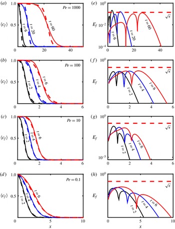
(a–d) Average concentration profiles
 $\langle c_{f}\rangle$
along the channel obtained either from the upscaled 1D (solid lines) or the pore-scale 2D equations (dashed lines) for different instances in time and Péclet numbers, i.e.
 $Pe=\{0.1,10,100,1000\}$
. (e–h) Absolute error
 $E_{f}(x,t):=|\langle c_{f}\rangle _{2D}-\langle c_{f}\rangle _{1D}|$
corresponding to each simulation. The dashed horizontal line represents the error bound
 $\sqrt{{\it\epsilon}}$
prescribed by homogenization theory. As predicted, the 1D equations capture the pore-scale dynamics within errors of order
 $\sqrt{{\it\epsilon}}$
for
 $Pe<{\it\epsilon}^{-1/2}\approx 7$
. Importantly, for
 $10<Pe<100$
, the 1D simulation is still accurate. For
 $Pe=1000$
, the error is not bounded by
 $\sqrt{{\it\epsilon}}$
at early times, but the 1D model accuracy is recovered at later times. The simulation parameters are
 ${\it\epsilon}=0.02$
,
 ${\it\lambda}=10$
,
 ${\it\Psi}=-0.78$
,
 ${\it\phi}=0.1$
,
 $D_{f}=1$
,
 $D_{mx}=0.1$
,
 $D_{my}=0.1$
and
 $h=10$
.

In figure 6, we compare the averaged fully resolved two-dimensional and the upscaled approximated solutions
 $\langle c_{f}\rangle _{2D}(x,t)$
and
 $\langle c_{f}\rangle _{1D}(x,t)$
respectively for different values of the Péclet number,
 $Pe=\{0.1,10,100,1000\}$
, and porosity,
 ${\it\phi}=\{0.01,0.1\}$
, and plot the absolute error
 $E_{f}(x,t):=|\langle c_{f}\rangle _{2D}-\langle c_{f}\rangle _{1D}|$
. The simulations in figure 6 are run for
 ${\it\epsilon}=0.02$
,
 ${\it\lambda}=10$
and
 ${\it\phi}=0.1$
.
In figure 6, we show that the absolute error between the 2D and 1D models decreases with increasing time and distance from the inlet for all scenarios. More specifically, the macroscopic 1D model performs within the expected accuracy for
 $Pe<{\it\epsilon}^{-1/2}$
(
 ${\approx}7$
for
 ${\it\epsilon}=0.02$
), i.e.
 $E_{f}(x,t)$
is bounded by
 $\sqrt{{\it\epsilon}}$
, see figure 6(d,h). The error bound is satisfied even when the constraints on the Péclet number are relaxed, i.e.
 $O({\it\epsilon}^{-1/2})\leqslant Pe\leqslant O({\it\epsilon}^{-1})$
, or
 $10\leqslant Pe\leqslant Pe^{\star }$
in figures 6(b,f) and (c,g). This result highlights that the conditions (1) and (2) are sufficient, but not necessary, to guarantee that error bounds prescribed by homogenization theory are realized. For
 $Pe>O({\it\epsilon}^{-1})$
(or
 $Pe>Pe^{\star }$
),
 $E_{f}(x,t)>\sqrt{{\it\epsilon}}$
for early times; the 1D model regains its accuracy at late (dimensionless) times
 $t>{\it\epsilon}Pe$
, i.e.
 $t>20$
in figure 6(a,e).
Simulation parameters:
 ${\it\epsilon}=0.02$
,
 ${\it\lambda}=31.6$
,
 ${\it\phi}=0.1$
,
 ${\it\Psi}=-0.78$
,
 $D_{f}=1$
,
 $D_{mx}=0.1$
,
 $D_{my}=0.1$
,
 $h=10$
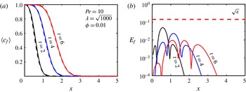
. (a) Average concentration profiles
 $\langle c_{f}\rangle$
along the channel obtained either from the upscaled 1D (solid lines) or from the pore-scale 2D equations (dashed lines) for different instances in time. (b) Absolute error
 $E_{f}(x,t):=|\langle c_{f}\rangle _{2D}-\langle c_{f}\rangle _{1D}|$
corresponding to each simulation. The dashed horizontal line represents the error bound
 $\sqrt{{\it\epsilon}}$
prescribed by homogenization theory.

In figure 7, we plot the profiles of the average concentration in the channel obtained from the numerically averaged 2D equations and the 1D upscaled equations. The simulations are run for
 ${\it\lambda}=31.6$
and
 ${\it\phi}=0.1$
. The error between the microscale and macroscale equations, figure 7(b), is lower compared with the scenario with the same Péclet number and higher permeability and porosity, specifically figure 6(c,g). This is consistent with the upscaling approach, where higher-order terms in the transverse direction are neglected, thus leading to increased error for a highly permeable matrix.
To further investigate the accuracy of the upscaled equations in different regimes and the temporal dependence of the error, we plot the solute breakthrough curves at a given location
 $x=x^{\star }$
along the channel.
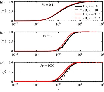
Time evolution of the channel average concentration
 $\langle c_{f}\rangle$
calculated at location
 $x^{\star }=b$
for different
 ${\it\lambda}$
and Péclet numbers. The parameters used in the simulations are
 ${\it\phi}=0.01$
,
 ${\it\Psi}=-0.78$
,
 ${\it\epsilon}=0.01$
,
 $D_{f}=1$
and
 $h=10$
.

In figure 8, we plot the concentration profile for three Péclet numbers and two values of the dimensionless permeability,
 ${\it\lambda}=\sqrt{10^{2}}$
and
 ${\it\lambda}=\sqrt{10^{3}}$
. For
 $Pe\ll 1$
, there is an excellent agreement between the upscaled and two-dimensional solutions for all times and both permeability values. The match is within the expected error bounds, figure 8(a). For higher Péclet numbers,
 $Pe=1$
(figure 8
b) and
 $Pe=1000$
(figure 8
c), the upscaled solution can still capture the averaged pore-scale concentration despite the fact that condition (2) is violated for
 $Pe=1000$
. Good performance of the model in regimes where (2) is violated can be expected since such a constraint is simply a sufficient (and not necessary) condition to guarantee that the upscaled equation (3.5) describes spatially averaged pore-scale processes within errors of order
 $\sqrt{{\it\epsilon}}$
. For
 $Pe=1000$
the match between the upscaled and the averaged pore-scale solution improves at later times. Since condition (2) is violated, the transient terms in the expansion, specifically
 $\partial _{t}c_{f}^{(0)}$
and
 $\partial _{t}c_{m}^{(0)}$
in (A 3a
), are not negligible and should be accounted for at the leading order. Failing to do so yields to a slightly higher approximation error, which decreases in time as the solution approaches the steady state and the transient terms become increasingly small, i.e.
 $\partial _{t}c_{f}^{(0)}\rightarrow 0$
and
 $\partial _{t}c_{m}^{(0)}\rightarrow 0$
as
 $t\rightarrow \infty$
.
5.3 Upscaled model results
Difference between the average concentration in the channel
 $\langle c_{f}\rangle$
for two values of the dimensionless permeability,
 ${\it\lambda}=\sqrt{10^{2}}$
and
 ${\it\lambda}=\sqrt{10^{3}}$
, and different Péclet numbers, obtained from (3.5). The set of parameters used in the simulations is
 ${\it\phi}=0.5$
,
 ${\it\Psi}=-0.78$
,
 ${\it\epsilon}=0.02$
,
 $D_{f}=1$
,
 $D_{mx}=0.1$
,
 $D_{my}=0.1$
,
 $h=10$
. The concentration
 $\langle c_{f}\rangle$
is measured at
 $x=1$
.

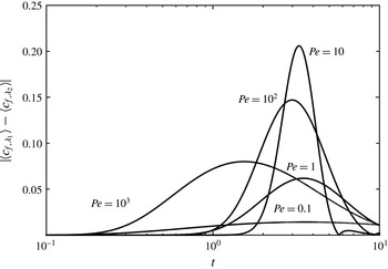
Figure 9 shows the difference between the average concentrations in the channel calculated from (3.5) for two values of
 ${\it\lambda}$
,
 ${\it\lambda}=\sqrt{10^{2}}$
and
 ${\it\lambda}=\sqrt{10^{3}}$
, at a given location along the channel, and for different Péclet numbers. Figure 9 shows how differences in matrix permeability become more relevant for intermediate Péclet numbers, i.e.
 $Pe\in (1,Pe^{\star })$
, when the interplay between advective and diffusive mass transfer is strongly controlled by the matrix properties. For
 $Pe<1$
, diffusive transport is dominant. In this scenario, the geometrical characteristics of the matrix have a small impact on transport. Similarly, for
 $Pe>Pe^{\star }$
, the impact of the matrix permeability decreases. In advection-dominated regimes, the concentration reaches saturation (
 $c_{f}=1$
) in a short period of time. This leads to a weak dependence of the macroscale concentration on the matrix topological features.
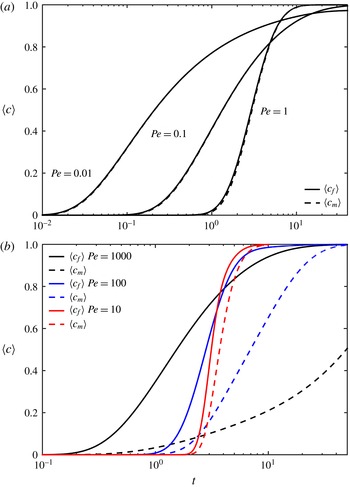
Figure 10 shows the temporal evolution of the macroscopic concentration in the channel and the matrix at a given location along the flow direction. In diffusion-dominated regimes, i.e. when
 $Pe<1$
, figure 10(a), the concentration difference in the matrix and the channel is very small. Fast diffusive mass transport enhances transverse mixing at the interface between the matrix and the channel, and leads to decreased differences in concentration between the former and the latter. For high Péclet numbers, figure 10(b), the difference in the average concentrations in the matrix and the channel increases due to the delay in advective mass transfer in the matrix. As a result, the concentration gradient, and therefore the mass flux, across the matrix–channel interface increases with
 $Pe$
for a given permeability value.
Comparison between
 $\langle c_{f}\rangle$
(solid lines) and
 $\langle c_{m}\rangle$
(dashed lines) for low (a) and high Péclet numbers (b). The simulation parameters are
 ${\it\phi}=0.5$
,
 ${\it\Psi}=-0.78$
,
 ${\it\epsilon}=0.02$
,
 $D_{f}=1$
,
 $D_{mx}=0.1$
,
 $D_{my}=0.1$
,
 $h=10$
. The concentrations
 $\langle c_{f}\rangle$
and
 $\langle c_{m}\rangle$
are measured at
 $x=1$
.

5.4 Comparison with existing models
In this section, we compare the proposed model with that introduced by Dejam et al., who assume that mass transport in the porous matrix is purely diffusive and transverse to flow (i.e.
 $y$
-direction). This corresponds to the
 $k=0$
(or
 ${\it\lambda}\rightarrow \infty$
) limit in the present model. To analyse differences and/or similarities in performance between the two models, we consider two configurations: a highly permeable (
 ${\it\lambda}=0.3$
) and a nearly impermeable (
 ${\it\lambda}=100$
) matrix. Dejam et al.’s solution for the average concentration in the fracture,
 $\langle c\rangle _{f,DHC}$
, is (Dejam et al.
Reference Dejam, Hassanzadeh and Chen2014)
 $$\begin{eqnarray}\langle c\rangle _{f,DHC}(x,t_{D})=\frac{\text{e}^{{\it\alpha}t_{D}}}{t_{D}}\left\{\frac{1}{2}{\hat{C}}_{f,DHC}(x,{\it\alpha})+Re\left[\mathop{\sum }_{l=1}^{n}(-1)^{l}{\hat{C}}_{f,DHC}\left(x,{\it\alpha}+\frac{l{\rm\pi}}{t_{D}}\sqrt{-1}\right)\right]\right\},\end{eqnarray}$$
where
 $Re[\cdot ]$
represents the real part of a complex function,
 ${\it\alpha}$
controls the accuracy of the numerical Laplace transform and
 $t_{D}=\tilde{t}/(b^{2}/D_{my})$
. In the following comparative study, we use the dimensionless time defined in (3.2) instead. Moreover, we set
 ${\it\alpha}t_{D}=4$
and use
 $n=1e5$
terms in the summation.
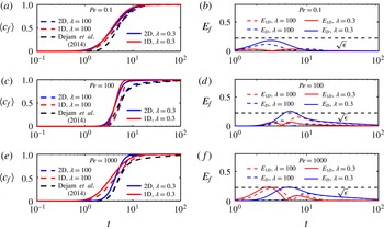
(a,c,e) Comparison between the breakthrough curves obtained from (3.5a
) and (5.2) (by Dejam et al.) and the averaged pore-scale solution for two permeability values,
 ${\it\lambda}=0.3$
and
 ${\it\lambda}=100$
. (b,d,f) Absolute errors between the upscaled solutions (3.5a
) and (5.2) and the averaged pore-scale solution,
 $E_{1D}(x,t;{\it\lambda}):=|\langle c_{f}\rangle _{2D}-\langle c\rangle _{f,1D}|$
and
 $E_{D}(x,t;{\it\lambda}):=|\langle c_{f}\rangle _{2D}-\langle c\rangle _{f,Dejam~et~al.}|$
respectively. The simulation parameters are
 ${\it\epsilon}=0.02$
,
 ${\it\phi}=0.1$
,
 ${\it\Psi}=-1$
,
 $D_{f}=1$
,
 $D_{mx}=0.1$
,
 $D_{my}=0.01$
and
 $h=10$
.

In figure 11, we compare the models (3.5a
) and (5.2) (by Dejam et al.) with the macroscopic concentration obtained from averaging the pore-scale solution. For low Péclet numbers, both models perform well independently of the matrix permeability. For high Péclet number (
 $Pe=100$
) and low permeability (or high
 ${\it\lambda}$
), Dejam et al.’s solution shows a better accuracy than the upscaled model proposed here. This is apparent from the error
 $E_{f}$
plotted in figure 11 as a function of time: while model (3.5a
) can still be considered to be predictive since
 $E_{f}$
is bounded by
 $\sqrt{{\it\epsilon}}$
, Dejam et al.’s solution has a lower maximum error. Conversely, for
 $Pe=100$
and high permeability values (or low
 ${\it\lambda}$
), our upscaled equation (3.5a
) is more accurate than (5.2). Importantly, in this scenario, the error in Dejam et al.’s solution is not bounded by
 $\sqrt{{\it\epsilon}}$
, i.e. the error is larger than that prescribed by the upscaling procedure. Finally, for very large
 $Pe$
(
 $Pe=1000$
), both models give higher errors at early times, regardless of the permeability value. This analysis demonstrates that the model described by (3.5a
) and Dejam et al.’s solution are complementary to each other, since the former can accurately describe macroscopic mass transport in advection-dominated regimes in coupled systems with highly permeable matrices, while the latter captures transverse diffusion into the matrix only in the low-permeability case.
6 Conclusions
Flow and transport above micro-patterned and porous surfaces occur in a variety of systems, ranging from engineered surfaces to bioreactor devices. The achievement of optimal macroscopic properties, e.g. improved mixing, in a number of such applications is hampered by the lack of understanding of how surface/matrix properties (e.g. porosity, permeability and thickness) relate to the system or macroscale.
In this work, we use perturbation methods to study passive scalar transport in a coupled channel–matrix system and obtain an analytical relationship between matrix properties and solute transverse dispersion. To the best of our knowledge, this is the first analytical relationship that establishes a connection between macroscopic transport features, matrix properties and transport regimes (i.e. Péclet number). We accomplish this by deriving upscaled equations for mass transport in a channel–matrix coupled system, while accounting for two-dimensional diffusion and a non-uniform velocity field both in the channel and in the matrix. The average velocity profile in the coupled system, as well as the slip velocity at the channel–matrix interface, is determined by a two-domain approach where the Stokes and Darcy–Brinkman equations are coupled to describe flow in the channel and in the permeable matrix respectively.
Our results show that the impact of matrix properties on solute transverse mixing, and, more specifically, on the macroscopic dispersion coefficient, is controlled by the magnitude of the Péclet number. In particular, for
 $Pe<1$
, transport in the channel–matrix system is dominated by diffusion, and the matrix properties have little to no impact on macroscopic transport. In this regime, mixing is controlled by diffusion in the direction transverse to the mean flow, and the dimensionless dispersion coefficient is independent of both
 $Pe$
and the matrix permeability. When
 $1<Pe<Pe^{\star }$
, solute transport is controlled by both diffusion and advection. The interplay between these mass transport mechanisms is strongly dependent on both the matrix permeability and the Péclet number. In this regime, macroscale dispersion can be controlled by both active and passive mechanisms. The former consist in modifying the operating flow conditions of the device (i.e. Péclet number), while the latter are based on modifying the surface coating properties (i.e. permeability). For
 $Pe>Pe^{\star }$
, mass transport is dominated by advection, and the dispersion coefficient reaches a constant value independent of the Péclet number and a function of the matrix permeability only. By means of asymptotic analysis, we demonstrate that different scaling regimes of the normalized dispersion coefficient
 ${\it\Pi}$
exist for thin (
 ${\it\Lambda}\lesssim 1$
) and thick porous layers (
 ${\it\Lambda}\gg 1$
). In particular,
 ${\it\Pi}$
is controlled by the dimensionless width
 $h$
of the porous matrix, when
 ${\it\Lambda}\lesssim 1$
, and scales linearly or quadratically with
 $h$
, when
 $h<1$
or
 $h>1$
respectively. In the thick-porous-medium regime,
 ${\it\Pi}$
is controlled by the matrix permeability
 ${\it\lambda}$
. This provides specific design guidelines to optimize mixing in channel–porous systems.
The upscaled model was validated against numerical simulations of the fully resolved two-dimensional channel–matrix coupled system. The upscaled solution agrees with the average concentration obtained from the exact two-dimensional ADEs within the error bound prescribed by the homogenization approach and performs well for large
 $Pe$
, despite the fact that condition (2) is violated. This is to be expected since the latter is a sufficient (and not necessary) condition to guarantee that the upscaled equation (3.5) describes spatially averaged pore-scale processes within errors of order
 $\sqrt{{\it\epsilon}}$
.
Finally, a detailed comparison between our model and that of Dejam et al. (Reference Dejam, Hassanzadeh and Chen2014), which only considers one-dimensional transverse diffusion in the matrix, shows that the two models are complementary to each other. For systems with permeable matrices, we found our model to be superior to Dejam et al.’s for all considered Péclet numbers. Conversely, unlike Dejam et al.’s model, our model cannot accurately capture the tailing effect introduced by the purely diffuse interfacial mass flux in impermeable matrices.
To the best of our knowledge, this is the first study that provides (i) a rigorous basis to relate the matrix permeability to the dispersion coefficient in coupled channel–matrix systems and (ii) quantitative guidelines for the design of porous/micro-patterned surfaces. The analysis also shows the possibility of controlling dispersion by either active (i.e. changing the operating conditions) or passive mechanisms (i.e. controlling the matrix properties) in the appropriate range of Péclet numbers.
Acknowledgements
I.B. gratefully acknowledges partial support by the US Department of Energy (DOE), Office of Biological and Environmental Research, Subsurface Biogeochemical Research (SBR) Program through the SBR Scientific Focus Area at PNNL, and the National Science Foundation (NSF) through the award no. 1533874, ‘DMREF: an integrated multiscale modelling and experimental approach to design fouling resistant membranes’. A.M.T. was partially supported by the US Department of Energy (DOE) Office of Advanced Scientific Computing (ASCR) as part of the Early Career Award ‘New Dimension Reduction Methods and Scalable Algorithms for Multiscale Nonlinear Phenomena’ and DOE’s Office of Biological and Environmental Research (BER) through the Pacific Northwest National Laboratory (PNNL) Subsurface Biogeochemical Research Scientific Focus Area project. PNNL is operated by Battelle for the DOE under Contract DE-AC05-76RL01830.
Appendix A. Asymptotic expansion
Substituting (3.4) into (3.2a ) and (3.2b ) leads to
 $$\begin{eqnarray}\displaystyle & & \displaystyle {\it\epsilon}^{1-{\it\alpha}}\left(\frac{\partial c_{f}^{(0)}}{\partial t}+\sqrt{{\it\epsilon}}\frac{\partial c_{f}^{(1)}}{\partial t}+{\it\epsilon}\frac{\partial c_{f}^{(2)}}{\partial t}\right)+{\it\epsilon}^{1/2-{\it\alpha}}\left(u_{f}\frac{\partial c_{f}^{(0)}}{\partial {\it\xi}}+\sqrt{{\it\epsilon}}u_{f}\frac{\partial c_{f}^{(1)}}{\partial {\it\xi}}+{\it\epsilon}u_{f}\frac{\partial c_{f}^{(2)}}{\partial {\it\xi}}\right)\nonumber\\ \displaystyle & & \displaystyle \quad ={\it\epsilon}D_{f}\left(\frac{\partial ^{2}c_{f}^{(0)}}{\partial {\it\xi}^{2}}+\sqrt{{\it\epsilon}}\frac{\partial ^{2}c_{f}^{(1)}}{\partial {\it\xi}^{2}}+{\it\epsilon}\frac{\partial ^{2}c_{f}^{(2)}}{\partial {\it\xi}^{2}}\right)+D_{f}\left(\sqrt{{\it\epsilon}}\frac{\partial ^{2}c_{f}^{(1)}}{\partial y^{2}}+{\it\epsilon}\frac{\partial ^{2}c_{f}^{(2)}}{\partial y^{2}}\right)\end{eqnarray}$$
and
 $$\begin{eqnarray}\displaystyle & & \displaystyle {\it\epsilon}^{1-{\it\alpha}}\left(\frac{\partial c_{m}^{(0)}}{\partial t}+\sqrt{{\it\epsilon}}\frac{\partial c_{m}^{(1)}}{\partial t}+{\it\epsilon}\frac{\partial c_{m}^{(2)}}{\partial t}\right)+{\it\epsilon}^{1/2-{\it\alpha}}\left(u_{m}\frac{\partial c_{m}^{(0)}}{\partial {\it\xi}}+\sqrt{{\it\epsilon}}u_{m}\frac{\partial c_{m}^{(1)}}{\partial {\it\xi}}+{\it\epsilon}u_{m}\frac{\partial c_{m}^{(2)}}{\partial {\it\xi}}\right)\nonumber\\ \displaystyle & & \displaystyle \quad ={\it\epsilon}D_{mx}\left(\frac{\partial ^{2}c_{m}^{(0)}}{\partial {\it\xi}^{2}}+\sqrt{{\it\epsilon}}\frac{\partial ^{2}c_{m}^{(1)}}{\partial {\it\xi}^{2}}+{\it\epsilon}\frac{\partial ^{2}c_{m}^{(2)}}{\partial {\it\xi}^{2}}\right)+D_{my}\left(\sqrt{{\it\epsilon}}\frac{\partial ^{2}c_{m}^{(1)}}{\partial y^{2}}+{\it\epsilon}\frac{\partial ^{2}c_{m}^{(2)}}{\partial y^{2}}\right)\end{eqnarray}$$
respectively. Given
 ${\it\alpha}<1/2$
, we collect terms of like power of
 ${\it\epsilon}$
as follows:
 $$\begin{eqnarray}\displaystyle & & \displaystyle \sqrt{{\it\epsilon}}\left({\it\epsilon}^{-{\it\alpha}}u_{f}\frac{\partial c_{f}^{(0)}}{\partial {\it\xi}}-D_{f}\frac{\partial ^{2}c_{f}^{(1)}}{\partial y^{2}}\right)+{\it\epsilon}\left({\it\epsilon}^{-{\it\alpha}}\frac{\partial c_{f}^{(0)}}{\partial t}+{\it\epsilon}^{-{\it\alpha}}u_{f}\frac{\partial c_{f}^{(1)}}{\partial {\it\xi}}-D_{f}\frac{\partial ^{2}c_{f}^{(0)}}{\partial {\it\xi}^{2}}-D_{f}\frac{\partial ^{2}c_{f}^{(2)}}{\partial y^{2}}\right)\nonumber\\ \displaystyle & & \displaystyle \quad +\,{\it\epsilon}\sqrt{{\it\epsilon}}\left({\it\epsilon}^{-{\it\alpha}}\frac{\partial c_{f}^{(1)}}{\partial t}+{\it\epsilon}^{-{\it\alpha}}u_{f}\frac{\partial c_{f}^{(2)}}{\partial {\it\xi}}-D_{f}\frac{\partial ^{2}c_{f}^{(1)}}{\partial {\it\xi}^{2}}\right)=O({\it\epsilon}^{2}),\end{eqnarray}$$
 $$\begin{eqnarray}\displaystyle & & \displaystyle \sqrt{{\it\epsilon}}\left({\it\epsilon}^{-{\it\alpha}}u_{m}\frac{\partial c_{m}^{(0)}}{\partial {\it\xi}}-D_{my}\frac{\partial ^{2}c_{m}^{(1)}}{\partial y^{2}}\right)\nonumber\\ \displaystyle & & \displaystyle \quad +\,{\it\epsilon}\left({\it\epsilon}^{-{\it\alpha}}\frac{\partial c_{m}^{(0)}}{\partial t}+{\it\epsilon}^{-{\it\alpha}}u_{m}\frac{\partial c_{m}^{(1)}}{\partial {\it\xi}}-D_{mx}\frac{\partial ^{2}c_{m}^{(0)}}{\partial {\it\xi}^{2}}-D_{my}\frac{\partial ^{2}c_{m}^{(2)}}{\partial y^{2}}\right)\nonumber\\ \displaystyle & & \displaystyle \quad +\,{\it\epsilon}\sqrt{{\it\epsilon}}\left({\it\epsilon}^{-{\it\alpha}}\frac{\partial c_{m}^{(1)}}{\partial t}+{\it\epsilon}^{-{\it\alpha}}u_{m}\frac{\partial c_{m}^{(2)}}{\partial {\it\xi}}-D_{mx}\frac{\partial ^{2}c_{m}^{(1)}}{\partial {\it\xi}^{2}}\right)=O({\it\epsilon}^{2}).\end{eqnarray}$$
 $c_{j}^{(i)}$
. Specifically, for
 $c_{f}^{(i)}$
and
 $c_{m}^{(i)}$
we obtain
 $$\begin{eqnarray}\displaystyle & \displaystyle \frac{\partial ^{2}c_{f}^{(1)}}{\partial y^{2}}={\it\epsilon}^{-{\it\alpha}}\frac{u_{f}}{D_{f}}\frac{\partial c_{f}^{(0)}}{\partial {\it\xi}}, & \displaystyle\end{eqnarray}$$
 $$\begin{eqnarray}\displaystyle & \displaystyle {\it\epsilon}^{-{\it\alpha}}\frac{\partial c_{f}^{(0)}}{\partial t}+{\it\epsilon}^{-{\it\alpha}}u_{f}\frac{\partial c_{f}^{(1)}}{\partial {\it\xi}}=D_{f}\frac{\partial ^{2}c_{f}^{(0)}}{\partial {\it\xi}^{2}}+D_{f}\frac{\partial ^{2}c_{f}^{(2)}}{\partial y^{2}}, & \displaystyle\end{eqnarray}$$
 $$\begin{eqnarray}\displaystyle & \displaystyle {\it\epsilon}^{-{\it\alpha}}\frac{\partial c_{f}^{(1)}}{\partial t}+{\it\epsilon}^{-{\it\alpha}}u_{f}\frac{\partial c_{f}^{(2)}}{\partial {\it\xi}}=D_{f}\frac{\partial ^{2}c_{f}^{(1)}}{\partial {\it\xi}^{2}} & \displaystyle\end{eqnarray}$$
 $$\begin{eqnarray}\displaystyle & \displaystyle \frac{\partial ^{2}c_{m}^{(1)}}{\partial y^{2}}={\it\epsilon}^{-{\it\alpha}}\frac{u_{m}}{D_{my}}\frac{\partial c_{m}^{(0)}}{\partial {\it\xi}}, & \displaystyle\end{eqnarray}$$
 $$\begin{eqnarray}\displaystyle & \displaystyle {\it\epsilon}^{-{\it\alpha}}\frac{\partial c_{m}^{(0)}}{\partial t}+{\it\epsilon}^{-{\it\alpha}}u_{m}\frac{\partial c_{m}^{(1)}}{\partial {\it\xi}}=D_{mx}\frac{\partial ^{2}c_{m}^{(0)}}{\partial {\it\xi}^{2}}+D_{my}\frac{\partial ^{2}c_{m}^{(2)}}{\partial y^{2}}, & \displaystyle\end{eqnarray}$$
 $$\begin{eqnarray}\displaystyle & \displaystyle {\it\epsilon}^{-{\it\alpha}}\frac{\partial c_{m}^{(1)}}{\partial t}+{\it\epsilon}^{-{\it\alpha}}u_{m}\frac{\partial c_{m}^{(2)}}{\partial {\it\xi}}=D_{mx}\frac{\partial ^{2}c_{m}^{(1)}}{\partial {\it\xi}^{2}} & \displaystyle\end{eqnarray}$$
 $$\begin{eqnarray}[c_{f}^{(0)}+\sqrt{{\it\epsilon}}c_{f}^{(1)}+{\it\epsilon}c_{f}^{(2)}]_{y=0}=[c_{m}^{(0)}+\sqrt{{\it\epsilon}}c_{m}^{(1)}+{\it\epsilon}c_{m}^{(2)}]_{y=0}\end{eqnarray}$$
and
 $$\begin{eqnarray}\left[\sqrt{{\it\epsilon}}\frac{\partial c_{f}^{(1)}}{\partial y}+{\it\epsilon}\frac{\partial c_{f}^{(2)}}{\partial y}\right]_{y=0}=\left[\sqrt{{\it\epsilon}}\frac{{\it\phi}D_{my}}{D_{f}}\frac{\partial c_{m}^{(1)}}{\partial y}+{\it\epsilon}\frac{{\it\phi}D_{my}}{D_{f}}\frac{\partial c_{m}^{(2)}}{\partial y}\right]_{y=0}.\end{eqnarray}$$
Matching like powers of
 ${\it\epsilon}$
in (A 7) leads to
 $$\begin{eqnarray}\displaystyle \left[\frac{\partial c_{f}^{(1)}}{\partial y}\right]_{y=0} & = & \displaystyle \frac{{\it\phi}D_{my}}{D_{f}}\left[\frac{\partial c_{m}^{(1)}}{\partial y}\right]_{y=0},\end{eqnarray}$$
 $$\begin{eqnarray}\displaystyle \left[\frac{\partial c_{f}^{(2)}}{\partial y}\right]_{y=0} & = & \displaystyle \frac{{\it\phi}D_{my}}{D_{f}}\left[\frac{\partial c_{m}^{(2)}}{\partial y}\right]_{y=0}.\end{eqnarray}$$
The cascade of equations (A 3) and (A 4) subject to the boundary conditions (A 6) and (A 8) can be solved iteratively.
Appendix B. Order
$O(\sqrt{{\it\epsilon}})$
:
$c_{f}^{(1)}$
and
$c_{m}^{(1)}$
solutions


Integrating equation (A 4a
) with respect to
 $y$
gives
 $$\begin{eqnarray}\frac{\partial c_{f}^{(1)}}{\partial y}=\frac{{\it\epsilon}^{-{\it\alpha}}}{D_{f}}\left(\int _{0}^{y}u_{f}\,\text{d}y+M_{1}\right)\frac{\partial c_{f}^{(0)}}{\partial {\it\xi}},\end{eqnarray}$$
where the integration constant
 $M_{1}$
is determined by using the no-flux condition (2.20) and the velocity profile (2.7),
 $$\begin{eqnarray}M_{1}=-\int _{0}^{1}u_{f}\,\text{d}y=-\!\left(\frac{{\it\Psi}}{6}+\frac{A}{2}+B\right),\end{eqnarray}$$
and
 $A$
and
 $B$
are defined in (2.9). Integration of (B 1) yields
 $$\begin{eqnarray}c_{f}^{(1)}=\frac{{\it\epsilon}^{-{\it\alpha}}}{D_{f}}\frac{\partial c_{f}^{(0)}}{\partial {\it\xi}}\left(M_{2}+M_{1}y+\iint _{0}^{y}u_{f}\,\text{d}^{2}y\right).\end{eqnarray}$$
By postulating
 $\langle c_{f}^{(1)}\rangle =0$
(Mikelic et al.
Reference Mikelic, Devigne and Duijn2006), we can solve for
 $M_{2}$
,
 $$\begin{eqnarray}M_{2}=-\!\left(\frac{{\it\Psi}}{120}+\frac{A}{24}+\frac{B}{2}+\frac{M_{1}}{2}\right).\end{eqnarray}$$
Inserting (B 4) and (B 2) in (B 3) leads to
 $$\begin{eqnarray}c_{f}^{(1)}=M(y)\frac{{\it\epsilon}^{-{\it\alpha}}}{D_{f}}\frac{\partial c_{f}^{(0)}}{\partial {\it\xi}},\end{eqnarray}$$
where
 $$\begin{eqnarray}M(y)=\frac{{\it\Psi}}{24}y^{4}+\frac{A}{6}y^{3}+\frac{B}{2}y^{2}+M_{1}y+M_{2}.\end{eqnarray}$$
Similarly, double integration of (A 5b
) yields a solution for
 $c_{m}^{(1)}$
in the following form:
 $$\begin{eqnarray}c_{m}^{(1)}=\frac{{\it\epsilon}^{-{\it\alpha}}}{D_{my}}N(y)\frac{\partial c_{m}^{(0)}}{\partial {\it\xi}},\end{eqnarray}$$
where
 $$\begin{eqnarray}N(y)=\frac{E}{{\it\lambda}^{2}}\text{e}^{{\it\lambda}y}+\frac{F}{{\it\lambda}^{2}}\text{e}^{-{\it\lambda}y}-\frac{{\it\Psi}}{2{\it\lambda}^{2}}y^{2}-\!\left(\frac{E}{{\it\lambda}}-\frac{F}{{\it\lambda}}\right)y+N_{1}y+N_{2}.\end{eqnarray}$$
Here,
 $E$
and
 $F$
are defined in (2.9) and
 $N_{1}$
and
 $N_{2}$
are integration constants. The constant
 $N_{1}$
is determined by imposing the boundary condition (2.20),
 $$\begin{eqnarray}N_{1}=\frac{E}{{\it\lambda}}(1-\text{e}^{-{\it\lambda}h})-\frac{F}{{\it\lambda}}(1-\text{e}^{-{\it\lambda}h})+\frac{{\it\Psi}h}{{\it\lambda}^{2}},\end{eqnarray}$$
and
 $N_{2}$
is determined by imposing
 $\langle c_{m}^{(1)}\rangle =0$
,
 $$\begin{eqnarray}N_{2}=-\!\left[\frac{E}{h{\it\lambda}^{3}}(1-\text{e}^{-{\it\lambda}h})-\frac{F}{h{\it\lambda}^{3}}(1-\text{e}^{{\it\lambda}h})-\frac{{\it\Psi}}{6{\it\lambda}^{2}}h^{2}+\frac{h}{2}\left(\frac{E}{{\it\lambda}}-\frac{F}{{\it\lambda}}\right)-\frac{N_{1}h}{2}\right].\end{eqnarray}$$
Equations (B 7), (B 9) and (B 10) fully define
 $c_{m}^{(1)}$
.
Appendix C. Order
$O({\it\epsilon})$
:
$c_{f}^{(2)}$
and
$c_{m}^{(2)}$
solutions


By inserting (B 5) into (A 4b ), we obtain
 $$\begin{eqnarray}{\it\epsilon}^{-{\it\alpha}}\frac{\partial c_{f}^{(0)}}{\partial t}+\frac{{\it\epsilon}^{-2{\it\alpha}}}{D_{f}}u_{f}M\frac{\partial ^{2}c_{f}^{(0)}}{\partial {\it\xi}^{2}}=D_{f}\frac{\partial ^{2}c_{f}^{(0)}}{\partial {\it\xi}^{2}}+D_{f}\frac{\partial ^{2}c_{f}^{(2)}}{\partial y^{2}},\end{eqnarray}$$
which provides an equation for
 $c_{f}^{(2)}$
. Averaging (C 1) gives
 $$\begin{eqnarray}{\it\epsilon}^{-{\it\alpha}}\frac{\partial c_{f}^{(0)}}{\partial t}+\frac{{\it\epsilon}^{-2{\it\alpha}}}{D_{f}}\langle u_{f}M\rangle \frac{\partial ^{2}c_{f}^{(0)}}{\partial {\it\xi}^{2}}=D_{f}\frac{\partial ^{2}c_{f}^{(0)}}{\partial {\it\xi}^{2}}-D_{f}\left[\frac{\partial c_{f}^{(2)}}{\partial y}\right]_{y=0}.\end{eqnarray}$$
Subtracting (C 2) from (C 1) yields
 $$\begin{eqnarray}\frac{{\it\epsilon}^{-2{\it\alpha}}}{D_{f}}(u_{f}M-\langle u_{f}M\rangle )\frac{\partial ^{2}c_{f}^{(0)}}{\partial {\it\xi}^{2}}=D_{f}\frac{\partial ^{2}c_{f}^{(2)}}{\partial y^{2}}+D_{f}\left[\frac{\partial c_{f}^{(2)}}{\partial y}\right]_{y=0},\end{eqnarray}$$
where the boundary term can be rewritten using (A 9). This leads to
 $$\begin{eqnarray}\frac{\partial ^{2}c_{f}^{(2)}}{\partial y^{2}}=\frac{{\it\epsilon}^{-2{\it\alpha}}}{D_{f}^{2}}(u_{f}M-\langle u_{f}M\rangle )\frac{\partial ^{2}c_{f}^{(0)}}{\partial {\it\xi}^{2}}-\frac{{\it\phi}D_{my}}{D_{f}}\left[\frac{\partial c_{m}^{(2)}}{\partial y}\right]_{y=0}.\end{eqnarray}$$
Integration in
 $y$
gives
 $$\begin{eqnarray}\frac{\partial c_{f}^{(2)}}{\partial y}=\frac{{\it\epsilon}^{-2{\it\alpha}}}{D_{f}^{2}}\frac{\partial ^{2}c_{f}^{(0)}}{\partial {\it\xi}^{2}}\int _{0}^{y}(u_{f}M-\langle u_{f}M\rangle )\,\text{d}y+\frac{{\it\phi}D_{my}}{D_{f}}\left[\frac{\partial c_{m}^{(2)}}{\partial y}\right]_{y=0}(K_{1}-y),\end{eqnarray}$$
where
 $K_{1}$
is an integration constant. Using the no-flux boundary condition at
 $y=1$
(2.20), while observing that
 $\int _{0}^{1}(u_{f}M-\langle u_{f}M\rangle )\,\text{d}y=\langle u_{f}M-\langle u_{f}M\rangle \rangle =0$
, yields
 $$\begin{eqnarray}K_{1}=1.\end{eqnarray}$$
Integrating (C 5) in
 $y$
once more leads to
 $$\begin{eqnarray}c_{f}^{(2)}=\frac{{\it\epsilon}^{-2{\it\alpha}}}{D_{f}^{2}}\frac{\partial ^{2}c_{f}^{(0)}}{\partial {\it\xi}^{2}}\iint _{0}^{y}(u_{f}M-\langle u_{f}M\rangle )\,\text{d}^{2}y+\frac{{\it\phi}D_{my}}{D_{f}}\left[\frac{\partial c_{m}^{(2)}}{\partial y}\right]_{y=0}\left(K_{2}+y-\frac{1}{2}y^{2}\right).\end{eqnarray}$$
Since
 $\langle c_{f}^{(2)}\rangle =0$
, then
 $$\begin{eqnarray}\int _{0}^{1}\left(K_{2}+y-\frac{1}{2}y^{2}\right)\,\text{d}y=0\quad \text{or }K_{2}=-\frac{1}{3}.\end{eqnarray}$$
Finally,
 $$\begin{eqnarray}c_{f}^{(2)}=\frac{{\it\epsilon}^{-2{\it\alpha}}}{D_{f}^{2}}\frac{\partial ^{2}c_{f}^{(0)}}{\partial {\it\xi}^{2}}\iint _{0}^{y}(u_{f}M-\langle u_{f}M\rangle )\,\text{d}^{2}y+\frac{{\it\phi}D_{my}}{D_{f}}\left[\frac{\partial c_{m}^{(2)}}{\partial y}\right]_{y=0}\left(-\frac{1}{2}y^{2}+y-\frac{1}{3}\right).\end{eqnarray}$$
A similar procedure leads to
 $$\begin{eqnarray}c_{m}^{(2)}=\frac{{\it\epsilon}^{-2{\it\alpha}}}{D_{my}^{2}}\frac{\partial ^{2}c_{m}^{(0)}}{\partial {\it\xi}^{2}}\iint _{0}^{y}(u_{m}N-\langle u_{m}N\rangle )\,\text{d}^{2}y+\frac{D_{f}}{{\it\phi}D_{my}}\left[\frac{\partial c_{f}^{(2)}}{\partial y}\right]_{y=0}\left(-\frac{1}{2}y^{2}-yh+\frac{1}{3}h^{2}\right).\end{eqnarray}$$
Appendix D. Upscaled equations
Applying the averaging operator to (A 1) and (A 2) while accounting for the third boundary condition (2.20) leads to
 $$\begin{eqnarray}\displaystyle & & \displaystyle \frac{\partial \langle c_{f}\rangle }{\partial t}+{\it\epsilon}^{-1/2}\langle u_{f}\rangle \frac{\partial c_{f}^{(0)}}{\partial {\it\xi}}+\left\langle u_{f}\frac{\partial c_{f}^{(1)}}{\partial {\it\xi}}\right\rangle +{\it\epsilon}^{-1/2}\left\langle u_{f}\frac{\partial c_{f}^{(2)}}{\partial {\it\xi}}\right\rangle \nonumber\\ \displaystyle & & \displaystyle \quad ={\it\epsilon}^{{\it\alpha}}D_{f}\frac{\partial ^{2}\langle c_{f}\rangle }{\partial {\it\xi}^{2}}-{\it\epsilon}^{{\it\alpha}-1/2}D_{f}\left[\frac{\partial c_{f}^{(1)}}{\partial y}\right]_{y=0}-{\it\epsilon}^{{\it\alpha}-1}D_{f}\left[\frac{\partial c_{f}^{(2)}}{\partial y}\right]_{y=0}\end{eqnarray}$$
and
 $$\begin{eqnarray}\displaystyle & & \displaystyle \frac{\partial \langle c_{m}\rangle }{\partial t}+{\it\epsilon}^{-1/2}\langle u_{m}\rangle \frac{\partial c_{m}^{(0)}}{\partial {\it\xi}}+\left\langle u_{m}\frac{\partial c_{m}^{(1)}}{\partial {\it\xi}}\right\rangle +{\it\epsilon}^{1/2}\left\langle u_{m}\frac{\partial c_{m}^{(2)}}{\partial {\it\xi}}\right\rangle \nonumber\\ \displaystyle & & \displaystyle \quad ={\it\epsilon}^{{\it\alpha}}D_{mx}\frac{\partial ^{2}\langle c_{m}\rangle }{\partial {\it\xi}^{2}}-{\it\epsilon}^{{\it\alpha}-1/2}\frac{D_{my}}{h}\left[\frac{\partial c_{m}^{(1)}}{\partial y}\right]_{y=0}-{\it\epsilon}^{{\it\alpha}-1}\frac{D_{my}}{h}\left[\frac{\partial c_{m}^{(2)}}{\partial y}\right]_{y=0}\end{eqnarray}$$
respectively, since
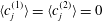 $\langle c_{j}^{(1)}\rangle =\langle c_{j}^{(2)}\rangle =0$
and
 $\langle c_{j}\rangle =\langle c_{j}^{(0)}\rangle$
, with
 $j=\{f,m\}$
. In order to close (D 1) and (D 2), the non-local advective terms and the boundary terms ought to be expressed in terms of macroscale quantities. Averaging (A 4c
) leads to
 $$\begin{eqnarray}\left\langle u_{f}\frac{\partial c_{f}^{(2)}}{\partial {\it\xi}}\right\rangle =0,\end{eqnarray}$$
since
 $\langle c_{f}^{(1)}\rangle =0$
. Inserting (B 5) in (D 1) while accounting for (D 3) gives
 $$\begin{eqnarray}\displaystyle & & \displaystyle \frac{\partial \langle c_{f}\rangle }{\partial t}+{\it\epsilon}^{-1/2}\langle u_{f}\rangle \frac{\partial c_{f}^{(0)}}{\partial {\it\xi}}+{\it\epsilon}^{-{\it\alpha}}{\displaystyle \frac{\langle u_{f}M\rangle }{D_{f}}}\frac{\partial ^{2}c_{f}^{(0)}}{\partial {\it\xi}^{2}}\nonumber\\ \displaystyle & & \displaystyle \quad ={\it\epsilon}^{{\it\alpha}}D_{f}\frac{\partial ^{2}\langle c_{f}\rangle }{\partial {\it\xi}^{2}}-{\it\epsilon}^{{\it\alpha}-1/2}D_{f}\left[\frac{\partial c_{f}^{(1)}}{\partial y}\right]_{y=0}-{\it\epsilon}^{{\it\alpha}-1}D_{f}\left[\frac{\partial c_{f}^{(2)}}{\partial y}\right]_{y=0}.\end{eqnarray}$$
Similarly, for the matrix we obtain
 $$\begin{eqnarray}\displaystyle & & \displaystyle \frac{\partial \langle c_{m}\rangle }{\partial t}+{\it\epsilon}^{-1/2}\langle u_{m}\rangle \frac{\partial c_{m}^{(0)}}{\partial {\it\xi}}+{\it\epsilon}^{-{\it\alpha}}\frac{\langle u_{m}N\rangle }{D_{my}}\frac{\partial ^{2}c_{m}^{(0)}}{\partial {\it\xi}^{2}}\nonumber\\ \displaystyle & & \displaystyle \quad ={\it\epsilon}^{{\it\alpha}}D_{mx}\frac{\partial ^{2}\langle c_{m}\rangle }{\partial {\it\xi}^{2}}-{\it\epsilon}^{{\it\alpha}-1/2}\frac{D_{my}}{h}\left[\frac{\partial c_{m}^{(1)}}{\partial y}\right]_{y=0}-{\it\epsilon}^{{\it\alpha}-1}\frac{D_{my}}{h}\left[\frac{\partial c_{m}^{(2)}}{\partial y}\right]_{y=0}.\end{eqnarray}$$
The last step to close (D 4) and (D 5) is to determine the boundary flux terms
 $[\partial _{y}c_{f}^{(1)}]_{y=0}$
and
 $[\partial _{y}c_{f}^{(2)}]_{y=0}$
. Combining the boundary condition (A 8) with (B 7) gives
 $$\begin{eqnarray}\frac{\partial c_{m}^{(1)}}{\partial y}={\it\epsilon}^{-{\it\alpha}}\frac{N^{\prime }}{D_{my}}\frac{\partial c_{m}^{(0)}}{\partial {\it\xi}},\end{eqnarray}$$
where
 $N^{\prime }=\text{d}N/\text{d}y$
and
 $[N^{\prime }]_{y=0}=N_{1}$
, see (B 8). Therefore,
 $$\begin{eqnarray}\left[\frac{\partial c_{m}^{(1)}}{\partial y}\right]_{y=0}={\it\epsilon}^{-{\it\alpha}}\frac{N_{1}}{D_{my}}\frac{\partial \langle c_{m}\rangle }{\partial {\it\xi}}.\end{eqnarray}$$
Combining (D 7) with (A 8) gives
 $$\begin{eqnarray}\left[\frac{\partial c_{f}^{(1)}}{\partial y}\right]_{y=0}={\it\epsilon}^{-{\it\alpha}}\frac{{\it\phi}N_{1}}{D_{f}}\frac{\partial \langle c_{m}\rangle }{\partial {\it\xi}}.\end{eqnarray}$$
Similarly, for the matrix,
 $$\begin{eqnarray}\left[\frac{\partial c_{m}^{(1)}}{\partial y}\right]_{y=0}={\it\epsilon}^{-{\it\alpha}}\frac{M_{1}}{{\it\phi}D_{my}}\frac{\partial \langle c_{f}\rangle }{\partial {\it\xi}}.\end{eqnarray}$$
From (C 9) we obtain
 $$\begin{eqnarray}\left[\frac{\partial c_{m}^{(2)}}{\partial y}\right]_{y=0}=-\frac{3D_{f}}{{\it\phi}D_{my}}c_{f}^{(2)}(y=0).\end{eqnarray}$$
At the interface
 $y=0$
, continuity of concentration (A 6) imposes
 $$\begin{eqnarray}{\it\epsilon}c_{m}^{(2)}=c_{f}^{(0)}-c_{m}^{(0)}+O(\sqrt{{\it\epsilon}})\quad \text{and}\quad {\it\epsilon}c_{f}^{(2)}=c_{m}^{(0)}-c_{f}^{(0)}+O(\sqrt{{\it\epsilon}}).\end{eqnarray}$$
Hence,
 $$\begin{eqnarray}\displaystyle & \displaystyle \left[\frac{\partial c_{m}^{(2)}}{\partial y}\right]_{y=0}=-\frac{3D_{f}}{{\it\phi}{\it\epsilon}D_{my}}(c_{f}^{(0)}-c_{m}^{(0)})=-\frac{3D_{f}}{{\it\phi}{\it\epsilon}D_{my}}(\langle c_{f}\rangle -\langle c_{m}\rangle ), & \displaystyle\end{eqnarray}$$
 $$\begin{eqnarray}\displaystyle & \displaystyle \left[\frac{\partial c_{m}^{(2)}}{\partial y}\right]_{y=0}=-\frac{3D_{f}}{{\it\phi}{\it\epsilon}D_{my}}(\langle c_{f}\rangle -\langle c_{m}\rangle ). & \displaystyle\end{eqnarray}$$
A similar relation can be found for the channel,
 $$\begin{eqnarray}\left[\frac{\partial c_{f}^{(2)}}{\partial y}\right]_{y=0}=\frac{3{\it\phi}D_{my}}{{\it\epsilon}hD_{f}}(\langle c_{f}\rangle -\langle c_{m}\rangle ).\end{eqnarray}$$
Inserting (D 8), (D 9), (D 12) and (D 14) into (D 4) and (D 5) gives
 $$\begin{eqnarray}\displaystyle & & \displaystyle \frac{\partial \langle c_{f}\rangle }{\partial t}+\frac{1}{\sqrt{{\it\epsilon}}}\langle u_{f}\rangle \frac{\partial \langle c_{f}\rangle }{\partial {\it\xi}}+\frac{{\it\epsilon}^{-{\it\alpha}}}{D_{f}}\langle u_{f}M\rangle \frac{\partial ^{2}\langle c_{f}\rangle }{\partial {\it\xi}^{2}}\nonumber\\ \displaystyle & & \displaystyle \quad ={\it\epsilon}^{{\it\alpha}}D_{f}\frac{\partial ^{2}\langle c_{f}\rangle }{\partial {\it\xi}^{2}}-{\it\epsilon}^{{\it\alpha}-1}\sqrt{{\it\epsilon}}{\it\phi}{\it\epsilon}^{-{\it\alpha}}N_{1}\frac{\partial \langle c_{m}\rangle }{\partial {\it\xi}}-{\it\epsilon}^{{\it\alpha}-1}\frac{3{\it\phi}D_{my}}{{\it\epsilon}h}(\langle c_{f}\rangle -\langle c_{m}\rangle )\end{eqnarray}$$
and
 $$\begin{eqnarray}\displaystyle & & \displaystyle \frac{\partial \langle c_{m}\rangle }{\partial t}+\frac{1}{\sqrt{{\it\epsilon}}}\langle u_{m}\rangle \frac{\partial \langle c_{m}\rangle }{\partial {\it\xi}}+\frac{{\it\epsilon}^{-{\it\alpha}}}{D_{my}}\langle u_{m}N\rangle \frac{\partial ^{2}\langle c_{m}\rangle }{\partial {\it\xi}^{2}}\nonumber\\ \displaystyle & & \displaystyle \quad ={\it\epsilon}^{{\it\alpha}}D_{mx}\frac{\partial ^{2}\langle c_{m}\rangle }{\partial {\it\xi}^{2}}+\frac{M_{1}}{{\it\phi}h\sqrt{{\it\epsilon}}}\frac{\partial \langle c_{f}\rangle }{\partial {\it\xi}}+{\it\epsilon}^{{\it\alpha}-1}\frac{D_{my}}{h}\frac{3D_{f}}{{\it\phi}{\it\epsilon}D_{my}}(\langle c_{f}\rangle -\langle c_{m}\rangle ).\end{eqnarray}$$
By rescaling the axis back to the physical coordinate
 $x$
, multiplying both sides by
 ${\it\epsilon}^{1-{\it\alpha}}$
and using the Péclet number definition, we obtain the macroscopic equations (3.5a
) and (3.5b
).