1. Introduction
Residual stress is a second-order unclosed term derived from the nonlinear convective flux in the averaged/filtered Navier–Stokes (N-S) equations, serving a crucial role in turbulence closure modelling and statistical analysis (Pope Reference Pope2011). In the context of Reynolds-averaged N-S equations (RANS) and large eddy simulation (LES), it manifests as Reynolds stress and subgrid-scale (SGS) stress. The statistical relationship between Reynolds stress and SGS stress illustrates the connection between these two types of turbulence modelling, which can support the construction of mode conversion in hybrid approaches, such as hybrid RANS/LES (Heinz Reference Heinz2020) and wall-modelled LES using RANS as the wall model (Bose & Park Reference Bose and Park2018).
Hybrid approaches are specifically designed to reduce the high computational cost of LES in high-Reynolds-number wall-bounded turbulence simulation, and are the currently available turbulence modelling methods in the aerospace engineering community. The flow close to the wall is characterised by small scales,
 $l^+ \sim \mathcal{O}(10^2)$
, causing LES of high-Reynolds-number flows to be unattainable to achieve fine resolution in the near-wall region (Bose & Park Reference Bose and Park2018). In this context, it is essential to implement a wall model within the near-wall region (Pradhan & Duraisamy Reference Pradhan and Duraisamy2023) or adjust the subgrid-scale stress to align with the statistical characteristics (Meneveau Reference Meneveau1994; Moser, Haering & Yalla Reference Moser, Haering and Yalla2021). Reynolds stress, representing the second statistical moment of velocity, serves as an effective natural wall model or benchmark for the adjustment of subgrid-scale stress within the near-wall region (Heinz Reference Heinz2020). The statistical relation between Reynolds stress and SGS stress can provide the coordination framework for the hybrid of RANS/LES and the stress modelling specification in the near-wall region. Using the statistical relationship between Reynolds stress and SGS stress, Xiao & Jenny (Reference Xiao and Jenny2012), Haering, Oliver & Moser (Reference Haering, Oliver and Moser2022), Mehta et al. (Reference Mehta, Manceau, Duffal and Meux2023) and Nguyen, Uribe & Afgan (Reference Nguyen, Uribe and Afgan2020) have implemented RANS models of Reynolds stress as a wall model to develop various hybrid RANS/LES methods. Through another route, Chen et al. (Reference Chen, Xia, Pei, Wang, Yang, Xiao and Shi2012) employed the statistical relation to constrain the SGS stress in the near-wall region, proposing a constrained large eddy simulation (CLES). By employing the residual stress relation, Verma, Park & Mahesh (Reference Verma, Park and Mahesh2013) proposed a novel dynamic SGS model featuring constrained SGS stress in the near-wall region. However, the statistical relation established in these studies assumes the filtering invariance of the averaged flow. Klein & Germano (Reference Klein and Germano2018) declared that this assumption fails when the averaged flow changes rapidly, such as in boundary layers, shear layers, shock waves, etc. They proposed an exact stress relation based on the commutativity of average and filter operators. Klein, Kasten & Germano (Reference Klein, Kasten and Germano2019) attempted to extend the relation to compressible flows, and he found that the difference between the residual stress derived from a Reynolds filter and that obtained from a Favre filter should be incorporated into the relation. Unfortunately, the stress relation that includes filter quantities in both senses is intractable for actual compressible turbulence modelling, as compressible modelling generally employs only the Favre filter quantity to avoid introducing additional unclosed terms. One solution is to construct the stress relation between Favre-averaged and Favre-filtered flow by using the aforementioned assumption. Jiang et al. (Reference Jiang, Xiao, Shi and Chen2013) and Bin et al. (Reference Bin, Xia, Shi, Zhang and Chen2021) extended CLES to compressible flows by using the assumption. Wang & Xiao (Reference Wang and Xiao2022) further extended CLES to compressible flow simulation with transition. Toki et al. (Reference Toki, Sousa, Chen and Scalo2024) adopted the same assumption to analyse the statistical relation of Reynolds stress and SGS stress in hypersonic Couette flow. Nonetheless, these studies of compressible turbulence modelling inevitably introduce additional physical assumptions.
To address the assumption limitations and applicable issues of the existing residual stress relation, this paper proposes a novel exact residual stress relation formula for compressible flow without introducing additional assumptions. The newly proposed relation can effectively establish the connection between the two compressible turbulence modelling methodologies of averaging and filtering frameworks. It will support the hybrid RANS/LES and LES with a wall-modelled constraint, as mentioned previously, appropriately extending to compressible flows. Compressible flows widely appear in aerospace engineering, and the finite-volume method (FVM) with unstructured mesh is widely used for complex engineering configurations. Therefore, to make the new stress relation formula beneficial for the engineering turbulence simulation community, this paper is carried out under the framework of the FVM. The detailed arrangement is as follows. Section 2.1 gives the stress relation formula for incompressible flow and then § 2.2 proposes the stress relation formula for compressible flow. Section 2.3 analyses the intrinsic filter of the FVM and presents a larger-scale filter based on the intrinsic filter to reflect the filter on a coarse mesh. In § 3, the new stress relation formula is verified by using channel turbulence with different Mach numbers and compressible boundary layer flow. Finally, § 4 concludes this work. In addition, to demonstrate the potential application of the residual stress relation in turbulence modelling, an example application for the hybrid RANS/LES method is given in the Appendix A.
2. Methodology
The definitions of several averaging and filtering operators are presented at the beginning. First is the averaging operator
 $\langle \ast \rangle$
, which commonly refers to ensemble averaging, known as the Reynolds average. In practice, the ensemble average is difficult to obtain. The time or spatial average can be used instead in stationary or homogeneous turbulence,
 \begin{equation} \langle Q\rangle (\boldsymbol{x},t) \triangleq \frac {1}{T} \int _{t-T}^{t+T} Q(\boldsymbol{x},\tau )\, {\textrm d}\tau \ ,\quad \langle Q\rangle (\boldsymbol{x},t) \triangleq \frac {1}{V_\varOmega } \int _{\varOmega } Q(\boldsymbol{r},t)\, {\textrm d}\boldsymbol{r} ,\end{equation}
where
 $T$
is the average period and
 $V_\varOmega$
is the homogeneous domain volume. In particular, homogeneity could be in a certain direction. The filter
 $\overline {\ast }$
is defined as a convolution,
 \begin{equation} \overline {Q}(\boldsymbol{x},t) \triangleq \int G(\boldsymbol{x}-\boldsymbol{y};\varDelta ) Q(\boldsymbol{y},t) \,{\textrm d}\boldsymbol{y}, \quad \textrm{where}\; \int G(\boldsymbol{x}-\boldsymbol{y},\varDelta )\, {\textrm d}\boldsymbol{y} = 1, \end{equation}
where
 $G(\boldsymbol{x}-\boldsymbol{y};\varDelta )$
is the filter kernel with filter scale
 $\varDelta$
. In FVM, there exists an intrinsic top-hat filter that is represented as an average over the mesh element, as detailed in § 2.3. For compressible flows, Favre averaging
 ${\langle \ast \rangle }_F$
and filtering
 $\widetilde {\ast }$
operators are widely used to address the issue of the non-distributivity of averaging and filtering operators over the product of density and velocity. They are defined as density-weighted averaging and filtering,
 \begin{equation} {\langle Q \rangle }_F \triangleq \langle \rho Q \rangle /\langle \rho \rangle , \quad \widetilde {Q} \triangleq \overline {\rho Q}/\overline {\rho }. \end{equation}
It is easy to verify that the five operators defined in (2.1), (2.2), (2.3) all have linear properties.
2.1. Residual stress statistical relation of incompressible flow
To establish the statistical relation between Reynolds stress and SGS stress, the filtering of Reynolds stress is considered. The following relation is obtained from the Reynolds stress definition
 $R_{\textit{ij}}=\langle u_i^\prime u_j^\prime \rangle$
(
 $u_i^\prime = u_i - \langle u_i \rangle$
) and the linear property of the averaging operator:
 \begin{equation} \overline {R}_{\textit{ij}}=\overline {\langle u_i^\prime u_j^\prime \rangle }=\overline {\langle u_iu_j\rangle -\langle u_i\rangle \langle u_j\rangle }. \end{equation}
The average and filter imply the following commutativity property (Klein & Germano Reference Klein and Germano2018):
 \begin{equation} \overline {\langle Q\rangle }=\langle \overline {Q}\rangle,\quad Q\rm{\ is\ an \ arbitrary\ flow\ quantity}. \end{equation}
Using the properties of commutativity and linearity, (2.4) can be rewritten as follows:
 \begin{equation} \overline {\langle u_i^\prime u_j^\prime \rangle }=\langle \overline { u_i u_j}\rangle -\langle \overline {u}_i\ \overline {u}_j\rangle +\langle \overline {u}_i\ \overline {u}_j\rangle -\langle \overline {u}_i\rangle \langle \overline {u}_j\rangle +\langle \overline {u}_i\rangle \langle \overline {u}_j\rangle -\overline {\langle u_i\rangle \langle u_j\rangle }. \end{equation}
The six terms on the right-hand side of (2.6) are paired by every two to form three components. The first component is the average of SGS stress
 $\tau _{\textit{ij}}$
. The second one (
 $T_{\textit{ij}}$
) is the Reynolds stress of filtered flow, which reflects the resolved part of Reynolds stress. The remaining one (
 $\nu _{\textit{ij}}$
) makes up the SGS stress of the mean flow, which can be obtained from the commutativity of average and filter operators,
 \begin{equation} \langle \tau _{\textit{ij}}\rangle =\langle \overline { u_i u_j}-\overline {u}_i\ \overline {u}_j\rangle ,\quad T_{\textit{ij}}=\langle \overline {u}_i\ \overline {u}_j\rangle -\langle \overline {u}_i\rangle \langle \overline {u}_j\rangle ,\quad \nu _{\textit{ij}}=\overline {\langle u_i\rangle \langle u_j\rangle }-\overline {\langle u_i\rangle }\ \overline {\langle u_j\rangle }. \end{equation}
Substituting (2.6) and (2.7) into (2.4), the following residual stress relation is obtained:
 \begin{equation} \overline {R}_{\textit{ij}}=\langle \tau _{\textit{ij}}\rangle + T_{\textit{ij}} - \nu _{\textit{ij}}. \end{equation}
It should be noted that although the derivation of relation (2.8) does not assume incompressible conditions, it is intractable for compressible turbulence modelling. Compressible turbulence modelling generally employs only the Favre-averaged quantity (
 ${\langle u_i \rangle }_F$
) and Favre-filtered quantity (
 $\tilde {u}_i$
) rather than Reynolds-averaged (
 $\langle u_i\rangle$
) and Reynolds-filtered quantities (
 $\overline {u}_i$
) to avoid introducing additional unclosed terms (Garnier, Adams & Sagaut Reference Garnier, Adams and Sagaut2009; Liu et al. Reference Liu, Zhou, Zhu and Wang2021; Griffin, Fu & Moin Reference Griffin, Fu and Moin2023). In addition, DNS simulations of compressible flows also often focus on Favre-averaged and Favre-filtered quantities (Wang et al. Reference Wang, Wan, Chen, Xie, Wang and Chen2019; Wenzel, Gibis & Kloker Reference Wenzel, Gibis and Kloker2022; Peng, Song & Xia Reference Peng, Song and Xia2024). Therefore, a new residual stress relation of the Favre average and filter is required for compressible flow.
2.2. Residual stress statistical relation of compressible flow
The key to deriving the residual stress relation in the previous section depends on the commutativity of the averaging and filtering operator, i.e. (2.5). However, Favre-averaging and Favre-filtering operators in compressible flow do not hold this property, i.e.
 $\widetilde {{\langle Q\rangle }_F} \neq {\langle \widetilde {Q}\rangle }_F$
. To obtain the statistical relation between Reynolds stress and SGS stress related to the Favre-average and Favre-filter quantities of compressible flow, the following two new averaging and filtering operators are defined:
 \begin{align}& \mathcal{F}(\ast ) \triangleq \overline {\langle \rho \rangle \ast }/\overline {\langle \rho \rangle } ,\end{align}
 \begin{align}& \mathcal{A}(\ast ) \triangleq \langle \overline {\rho }\ast \rangle /\langle \overline {\rho }\rangle. \end{align}
Here,
 $\mathcal{F}$
represents a weighted filter with the averaged density field as weight, which reflects the filtering of physical quantities modulated by the averaged density redistribution;
 $\mathcal{A}$
represents a weighted average with the filtered density field as weight, which reflects the averaging of physical quantities modulated by the filtered density field redistribution. It can be proved that the above-mentioned filtering and averaging operators satisfy the property of commutativity. The proof is shown in the following lemma.
Lemma 1. (Commutativity property) For any variable Q, the filter and average operators defined by ( 2.9 ) and ( 2.10 ) satisfy the following equation:
 \begin{equation} \mathcal{F}({\langle Q\rangle }_F) = \mathcal{A}(\widetilde {Q}). \end{equation}
Proof.
 \begin{align*} \rm{Left \ hand} & = \overline {\langle \rho \rangle {\langle Q\rangle }_F} \ / \ \overline {\langle \rho \rangle } = \overline {\langle \rho \rangle \ (\langle \rho Q\rangle \ / \ \langle \rho \rangle )} \ / \ \overline {\langle \rho \rangle } = \overline {\langle \rho Q \rangle } \ / \ \overline {\langle \rho \rangle },\\\rm{Right \ hand} & = \langle \overline {\rho } \widetilde {Q} \rangle \ / \ \langle \overline {\rho }\rangle = \langle \overline {\rho } \ (\overline {\rho Q} / \overline {\rho }) \rangle \ / \ \langle \overline {\rho }\rangle = \langle \overline {\rho Q} \rangle \ / \ \langle \overline {\rho }\rangle. \end{align*}
Using the commutativity property of the filter operator
 $\overline {\ast }$
and the average operator
 $\langle \ast \rangle$
in (2.5), the following equation can be obtained:
 \begin{align} \overline {\langle \rho Q \rangle } \ / \ \overline {\langle \rho \rangle } = \langle \overline {\rho Q} \rangle \ / \ \langle \overline {\rho }\rangle. \end{align}
And then,
 $\rm{left \ hand} = \rm{right \ hand}$
.
Lemma 1 clarifies a physical meaning that the Favre-averaged and Favre-filtered field converge to a unified physical quantity
 $\overline {\langle \rho Q \rangle } \ / \ \overline {\langle \rho \rangle }$
, namely the averaged-filtered conservation physical quantity
 $\rho Q$
per unit averaged-filtered density, after being acted upon by the
 $\mathcal{F}$
and
 $\mathcal{A}$
operators. The residual stress relation of compressible flow is derived as follows. Similarly, the Reynolds stress of compressible flow
 $R_{\textit{ij}}^C={\langle u_i^{\prime \prime } u_j^{\prime \prime }\rangle }_F$
(
 $u_i^{\prime \prime } = u_i - {\langle u_i \rangle }_F$
) is filtered first. Unlike the previous section, the filter operator defined in (2.9) is adopted here,
 \begin{equation} \mathcal{F}(R_{\textit{ij}}^C) = \mathcal{F}({\langle u_i^{\prime \prime } u_j^{\prime \prime }\rangle }_F)=\mathcal{F}({\langle u_iu_j\rangle }_F-{\langle u_i\rangle }_F{\langle u_j\rangle }_F). \end{equation}
Considering the linear properties of the filter operator
 $\mathcal{F}(\ast )$
and supplementing the corresponding moments of Favre filtering velocity defined by the new average operator
 $\mathcal{A}(\ast )$
, the following decomposition formula can be constructed:
 \begin{equation} \begin{aligned} \mathcal{F}({\langle u_i^{\prime \prime } u_j^{\prime \prime }\rangle }_F) & = \mathcal{F}({\langle u_iu_j\rangle }_F) - \mathcal{A}(\widetilde {u}_i\widetilde {u}_j) + \mathcal{A}(\widetilde {u}_i\widetilde {u}_j) - \mathcal{A}(\widetilde {u}_i)\mathcal{A}(\widetilde {u}_j) \\ &\quad + \mathcal{A}(\widetilde {u}_i)\mathcal{A}(\widetilde {u}_j) - \mathcal{F}({\langle u_i\rangle }_F{\langle u_j\rangle }_F). \end{aligned} \end{equation}
Reynolds stress of compressible flow can also be decomposed by three stress terms, which are obtained by pairing two adjacent terms of the six terms on the right-hand side of (2.14). According to lemma1, the first two terms on the right-hand side of (2.14) constitute the average of the subgrid-scale stress of compressible flow
 $\tau _{\textit{ij}}^C=\widetilde {u_iu_j}-\widetilde {u}_i\widetilde {u}_j$
,
 \begin{equation} \mathcal{A}(\tau _{\textit{ij}}^C) = \mathcal{A}(\widetilde {u_iu_j}) - \mathcal{A}(\widetilde {u}_i\widetilde {u}_j). \end{equation}
The third and fourth terms on the right-hand side of (2.14) constitute the Reynolds stress of the Favre-filtering field, which reflects the resolved Reynolds stress portion of the compressible flow,
 \begin{equation} T_{\textit{ij}}^C = \mathcal{A}(\widetilde {u}_i\widetilde {u}_j) - \mathcal{A}(\widetilde {u}_i)\mathcal{A}(\widetilde {u}_j). \end{equation}
The last two terms constitute the subgrid-scale stress of the mean flow, which can be obtained from lemma1,
 \begin{equation} \nu _{\textit{ij}}^C = \mathcal{F}({\langle u_i\rangle }_F{\langle u_j\rangle }_F) - \mathcal{F}({\langle u_i \rangle }_F)\mathcal{F}({\langle u_j \rangle }_F). \end{equation}
Finally, substituting (2.13), (2.22), (2.23) and (2.24) into (2.14), the statistical relation between Reynolds stress and SGS stress of compressible flow can be obtained. Figure 1 graphically shows the statistical relationship of the various stresses in (2.18). Here,
 $T_{\textit{ij}}^C$
and
 $\mathcal{A}(\tau _{\textit{ij}}^C)$
are derived from the filtered field,
 $\nu _{\textit{ij}}^C$
and
 $\mathcal{F}(R_{\textit{ij}}^C)$
are derived from the averaged field. They are correlated by the commutativity of the newly defined average and filter operators,
 \begin{equation} \mathcal{F}\left(R_{\textit{ij}}^C\right)=\mathcal{A}\left(\tau _{\textit{ij}}^C\right) + T_{\textit{ij}}^C - \nu _{\textit{ij}}^C. \end{equation}
Reynolds stress, as the second moment of fluctuation velocity, represents the momentum transfer caused by the turbulent fluctuation transport process. Turbulence is characterised by multiscale features, which means that the momentum transfer associated with Reynolds stress occurs across various scales. Equation (2.18) provides a decomposition of Reynolds stress on different scales, with each stress component representing a distinct physical process of momentum transfer (as shown in figure 2). Through filtering operations, turbulence is divided into two parts: the sup-filter scale larger than the filter scale and the sub-filter scale smaller than the filter scale. It is necessary to note that since (2.18) is decomposed using a general filter scale, the term ‘sub-filter scale’ is used here instead of the more typical ‘sub-grid scale’. When the grid scale aligns with the filter scale, these two terms are essentially equivalent. The first term on the right-hand side of (2.18) represents the average of the sub-filter stress, indicating the momentum transfer caused by turbulent transport at the sub-filter scale in the mean sense. This sub-filter scale turbulence momentum transfer can be divided into two contributions. One is the momentum transfer generated by the inhomogeneity of the average flow during the turbulent transport process, which is expressed as the sub-filter stress related to the average velocity, denoted as
 $\nu _{\textit{ij}}^C$
. The other arises from the turbulent fluctuations within the sub-filter scale, represented by the difference between
 $\tau _{\textit{ij}}^C$
and
 $\nu _{\textit{ij}}^C$
. However, the momentum transfer of the fluctuation flow (
 $\widetilde {u}_i^{\prime \prime }=\widetilde {u}_i-\mathcal{A}(\widetilde {u}_i)$
) in the turbulent transport process on the sup-filter scale can be expressed as the second moment of the filtered velocity, i.e.
 $T_{\textit{ij}}^C$
,
 \begin{equation} \mathcal{A}(\widetilde {u}_i^{\prime \prime }\widetilde {u}_j^{\prime \prime }) = \mathcal{A}(\widetilde {u}_i\widetilde {u}_j) - \mathcal{A}(\widetilde {u}_i)\mathcal{A}(\widetilde {u}_j)=T_{\textit{ij}}^C. \end{equation}
Additionally, the momentum transfer associated with turbulence fluctuations at the full scale is expressed as Reynolds stress. It can be related to the superposition of
 $\tau _{\textit{ij}}^C-\nu _{\textit{ij}}^C$
and
 $T_{\textit{ij}}^C$
by the average and filter operators in (2.10) and (2.9), appearing as the relation formula demonstrated in (2.18).
Statistical relation between averaged and filtered flow fields.

Schematic diagram of turbulent momentum transfer dominated by each stress component.

Turbulent heat flux, denoted as
 $q_{i}^t = {\langle h^{\prime \prime } u_i^{\prime \prime }\rangle }_F$
(
 $h^{\prime \prime } = h - {\langle h \rangle }_F$
), also plays a crucial role in compressible flow. It represents the second-order moment of fluctuations in enthalpy and velocity, illustrating the heat transfer processes associated with turbulent transport. Following the earlier discussion on the residual stress relation, the relationship between the turbulent heat flux of the averaged and filtered compressible flows can be derived. Similarly to (2.14), the following decomposition of turbulent heat flux can be derived by considering the definitions and linear properties of
 $\mathcal{F}(\ast )$
and
 $\mathcal{A}(\ast )$
:
 \begin{equation} \begin{aligned} \mathcal{F}({\langle h^{\prime \prime } u_i^{\prime \prime }\rangle }_F) & = \mathcal{F}({\langle hu_i\rangle }_F) - \mathcal{A}(\widetilde {h}\widetilde {u}_i) + \mathcal{A}(\widetilde {h}\widetilde {u}_i) - \mathcal{A}(\widetilde {h})\mathcal{A}(\widetilde {u}_i) \\ &\quad + \mathcal{A}(\widetilde {h})\mathcal{A}(\widetilde {u}_i) - \mathcal{F}({\langle h\rangle }_F{\langle u_i\rangle }_F). \end{aligned} \end{equation}
Then, the turbulent heat flux relation between averaged and filter compressible flow can be obtained by using lemma1,
 \begin{equation} \mathcal{F}(q_{i}^t)=\mathcal{A}(q_{sgs,i}) + S_{i} - \omega _{i}, \end{equation}
where
 $q_{sgs,i}$
,
 $S_{i}$
and
 $\omega _{i}$
on the right-hand side of (2.21) represent subgrid-scale turbulent heat flux, resolved heat flux and subgrid-scale heat flux of the mean flow, respectively, and their expressions are as follows:
 \begin{align} q_{sgs,i} =&\, \widetilde {hu_i} - \widetilde {h}\widetilde {u}_i, \end{align}
 \begin{align} S_{i} = \mathcal{A}(\widetilde {h}\widetilde {u}_i) &- \mathcal{A}(\widetilde {h})\mathcal{A}(\widetilde {u}_i), \end{align}
 \begin{align} \omega _{i} = \mathcal{F}({\langle h\rangle }_F{\langle u_i\rangle }_F) &- \mathcal{F}({\langle h \rangle }_F)\mathcal{F}({\langle u_i \rangle }_F). \end{align}
The turbulent heat flux and its decomposition formula resemble the mathematical form of residual stress. The heat flux decomposition formula effectively represents turbulent heat transfer across different scales of turbulence. In this context,
 $q_{i}^t$
refers to the heat transfer resulting from enthalpy fluctuations occurring in the full-scale turbulence transport process,
 $q_{sgs,i}$
represents the heat transfer associated with the turbulent transport of enthalpy at the sub-filter scale,
 $S_{i}$
refers to the heat transfer caused by the turbulent transport of enthalpy fluctuations at the sup-filter scale. Finally,
 $\omega _{i}$
indicates the heat transfer resulting from the inhomogeneity of the mean enthalpy in the turbulent transport at the sub-filter scale.
Residual stress decomposition establishes the relationship between Reynolds stress and subgrid-scale (SGS) stress, which is beneficial for the turbulence modelling of LES, especially in high-Reynolds-number wall-bounded flows. In high-Reynolds-number wall-bounded turbulence, due to computational cost limitation, LES modelling is often conducted on grids with inadequate resolution within the near-wall region. However, the direct application of LES on a grid with insufficient resolution will cause some non-physical issues due to the deficiency of SGS stress. To address the failure of SGS stress modelling caused by insufficient resolution on the coarse grid, the residual stress relation can be used to normalise the SGS stress in the insufficient resolution region. It is mainly reflected in the following three aspects.
-
(i) Using the residual stress relation to constrain the SGS stress near the wall, realising reasonable wall modelling.
-
(ii) Using the error of the residual stress relation formula as an objective function to dynamically optimise the coefficients of the SGS model, ensuring the SGS stress in the near-wall region is sufficient.
-
(iii) Applying the residual stress decomposition formula to appropriately adjust the SGS stress in the insufficient resolution region near the RANS/LES partition interface of the hybrid RANS/LES method, addressing the modelled stress deficiency issues of the transition between RANS and LES.
The first two methods were proposed by Chen et al. (Reference Chen, Xia, Pei, Wang, Yang, Xiao and Shi2012) and Verma et al. (Reference Verma, Park and Mahesh2013), respectively, using a simplified stress relation formula that ignores
 $ v_{\textit{ij}}$
. This paper presents the third application of residual stress relation in turbulence modelling. Specifically, a stress relation formula is used to effectively address the issues arising from inadequate resolution near the interface of the hybrid RANS/LES method. To maintain the consistency of the article, the details are presented in the Appendix A.
2.3. Filter operator of finite volume method
To promote the application of the proposed relation to the FVM method that is commonly used in engineering turbulence simulation, various filter operators are proposed under the framework of FVM. FVM has an intrinsic filter operator due to its natural formalism: the average operator on the mesh element. In the following, we will first present the explicit expression of the intrinsic filter, and then a filter operator on a larger scale will be proposed.
Applying Taylor expression to the centre of a mesh cell
 $\varOmega$
is as follows:
 \begin{equation} Q(\boldsymbol{x})=Q_c+(\boldsymbol{x}-\boldsymbol{x}_c)\boldsymbol{\cdot }\boldsymbol{\nabla } Q_c+(\boldsymbol{x}-\boldsymbol{x}_c)\otimes (\boldsymbol{x}-\boldsymbol{x}_c)\boldsymbol{:}\boldsymbol{\nabla }\circ \boldsymbol{\nabla } Q_c+rhs. \quad \boldsymbol{x}\in \varOmega. \end{equation}
The subscript
 $c$
represents the cell centre value,
 $\otimes$
represents the tensor product,
 $\boldsymbol{:}$
represents the double dot-product of the tensor and
 $\boldsymbol{\nabla }\circ \boldsymbol{\nabla }$
represents the second-order gradient of Q, i.e. Hessian matrix. The truncated order of gradients is determined by FVM solving accuracy. Second-order FVM expands to the first-order gradient, third-order FVM expands to the second-order gradient and so on. An explicit representation of FVM intrinsic filter
 $\overline {\ast }^\natural$
is obtained by averaging over cell
 $\varOmega$
,
 \begin{equation} \overline {Q}^\natural =Q_c+\frac {1}{V_\varOmega }\!\int _\varOmega \!(\boldsymbol{x}-\boldsymbol{x}_c)\,{\textrm d}\sigma \boldsymbol{\cdot }\boldsymbol{\nabla } Q_c+\frac {1}{\textit {V}_\varOmega }\!\int _\varOmega \!(\boldsymbol{x}-\boldsymbol{x}_c)\otimes (\boldsymbol{x}-\boldsymbol{x}_c)\,{\textrm d}\sigma \boldsymbol{:}\boldsymbol{\nabla }\circ \boldsymbol{\nabla } Q_c+\textit{rhs.}, \end{equation}
where
 $V_\varOmega$
is the cell volume. Equation (2.26) contains a series of integrals of the multi-product of
 $\boldsymbol{r}=\boldsymbol{x}-\boldsymbol{x}_c$
, which are only geometric quantities reflecting the filter scale. Moreover, the explicit expression of the k-order filter moment for n-order FVM can be given by the linear property,
 \begin{equation} \begin{aligned} & \overline {u_1{\cdots} u_k}^\natural =\sum _{m=0}^{kn-k}\sum _{i_1+{\cdots} +i_k=m}{\frac {1}{i_1!{\cdots} i_k!}\mathscr{A}\!\left\{\prod _{m}\boldsymbol{r}\!\right\}{\underbrace {\boldsymbol{\cdot }}_m}\!\left [\! \left(\!\prod _{i_1}\boldsymbol{\nabla }\!\right)\!u_1{\otimes {\cdots} \otimes }\!\left(\!\prod _{i_k}\boldsymbol{\nabla }\!\right) \!u_k \!\right ]_c} \\& \text{where} \; \mathscr{A}\left\{\prod _{m}\boldsymbol{r}\right\} \triangleq \frac {\int _\varOmega \prod _{m}\boldsymbol{r} {\textrm d}\sigma }{V_\varOmega } , \ \ \prod _{m}\boldsymbol{r} \triangleq \boldsymbol{r}\underbrace {\otimes {\cdots} \otimes }_m\boldsymbol{r} , \ \ \prod _{m}\boldsymbol{\nabla } \triangleq \boldsymbol{\nabla }\underbrace {\circ {\cdots} \circ }_m\boldsymbol{\nabla } ,\end{aligned} \end{equation}
where m-underbrace of dot-product in (2.27) denotes the m-order tensor dot-product. When m = 0, it is the scalar production. In addition, when m = 0,
 $\prod _{0}\boldsymbol{r} = 1$
, and
 $\prod _{0}\boldsymbol{\nabla } = \mathscr{I}$
is the identity operator. Using the intrinsic filter defined in (2.27), the corresponding intrinsic Favre filter
 $\widetilde {\ast }^\natural$
and the new filter
 $\mathcal{F}^{\natural }(\ast )$
defined in (2.9) can be obtained by replacing
 $\mathscr{A}\{\prod _{m}\boldsymbol{r}_c\}$
with the following formula:
 \begin{equation} \ \ \mathscr{A}_\rho \left\{\prod _{m}\boldsymbol{r}\right\} \triangleq \frac {\int _\varOmega \rho \prod _{m}\boldsymbol{r}\, {\textrm d}\sigma }{\int _\varOmega \rho \,{\textrm d}\sigma } , \quad \mathscr{A}_{\langle \rho \rangle }\left\{\prod _{m}\boldsymbol{r}\right\} \triangleq \frac {\int _\varOmega {\langle \rho \rangle }\prod _{m}\boldsymbol{r} \,{\textrm d}\sigma }{\int _\varOmega {\langle \rho \rangle }\, {\textrm d}\sigma }. \end{equation}
Further, the filter on a larger scale can be proposed from the above-mentioned intrinsic filter. A natural idea under the FVM framework is extending the neighbour schemes of the mesh cell to achieve a larger-scale averaging operation,
 \begin{equation} \overline {Q} \triangleq \frac {1}{V_\varOmega }\sum _{i\in \mathscr{N}}\int _{\varOmega _{i}}Q \,{\textrm d}\sigma = \sum _{i\in \mathscr{N}}{\overline {Q}^\natural }_i W_i , \quad W_i = \frac {V_{\varOmega _i}}{V_\varOmega }, \end{equation}
where
 $\mathscr{N}$
denotes the indicator set of the cell neighbour scheme,
 $V_{\varOmega _i}$
is the volume of the
 $i$
th cell in the neighbour scheme and
 $V_\varOmega$
is the total volume of the the neighbour scheme. Moreover, the corresponding other filters are proposed as follows:
 \begin{equation} \widetilde {Q} \triangleq \sum _{i\in \mathscr{N}}{\widetilde {Q}^\natural }_i \widetilde {W}_i, \quad \widetilde {W}_i = \frac {{\overline {\rho }^\natural }_i}{\overline {\rho }}W_i; \quad \mathcal{F}(Q) \triangleq \sum _{i\in \mathscr{N}}{\mathcal{F}^{\natural }(Q)}_i \widehat {W}_i, \quad \widehat {W}_i = \frac {{\overline {{\langle \rho \rangle }}^\natural }_i}{\overline {{\langle \rho \rangle }}}W_i. \end{equation}
3. Numerical experiment and verification
To verify the residual stress relation for compressible flow proposed in § 2, this section will examine it using channel flows with various Mach numbers (Ma) and supersonic turbulent boundary layer flow. The results data are derived from direct numerical simulation (DNS) of 3-D N-S equations using an in-house FVM-based compressible flow solver known as the hybrid unstructured 3-D N-S solver (HUNS3D) (Wang & Ye Reference Wang and Ye2004; Li, Sun & Wang Reference Li, Sun and Wang2024).
3.1. Compressible channel flow
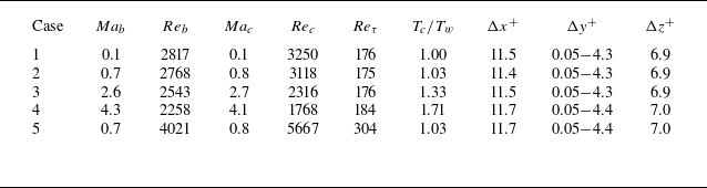
Channel flows with four Ma are investigated, and their corresponding Reynolds numbers (Re) and grid scales are detailed in table 1. The Mach number and Reynolds number at the centre of the channel are defined by the formulae
 $Ma_c \triangleq u_c/a_c$
and
 $Re_c \triangleq \rho _c u_c \delta /\mu _c$
, where
 $\rho _c$
,
 $u_c$
,
 $a_c$
,
 $\mu _c$
denote the density, velocity, sound speed and dynamic viscosity at the channel centre, and
 $\delta$
is the half-height of the channel. Here,
 $Re_\tau$
is the friction Reynolds number defined by the near-wall velocity scale
 $u_\tau \triangleq \sqrt {\tau _w / \rho _w}$
,
 $Re_\tau \triangleq u_\tau \delta / \nu _w$
, where
 $\tau _w$
,
 $\rho _w$
,
 $\nu _w$
denote the friction stress, density and kinematic viscosity coefficient at the wall. In addition, the bulk Mach number and Reynolds number are usually used for compressible channel turbulence (Yao & Hussain Reference Yao and Hussain2020), which are defined as
 $Ma_b \triangleq u_b/a_w$
and
 $Re_b \triangleq \rho _b u_b \delta /\mu _w$
, where
 $\rho _b$
is the bulk density,
 $u_b$
is the bulk velocity,
 $a_w$
is the sound speed at the wall and
 $\mu _w$
is the dynamic viscosity at the wall.
Case details of channel flows with different Mach numbers.

The computational domain dimensions in the streamwise, normal, spanwise directions are
 $4\pi \delta \times 2\delta \times 2\pi \delta$
. The number of grid points in the three directions is
 $192 \times 129 \times 160$
for
 $Re_\tau \approx 180$
and
 $320 \times 215 \times 267$
for
 $Re_\tau \approx 300$
. The grid in the streamwise and spanwise are distributed uniformly, while that in the normal direction are arranged using the formula
 $y_j = \cos (\theta _j)$
, where
 $\theta _j = (j-1)\pi /(N-1)$
for
 $j = 1, 2, \ldots , N$
. The grid adopted here is consistent with that of Kim et al. (Reference Kim, Moin and Moser1987). Non-slip isothermal boundary conditions are applied at the walls with periodic conditions for streamwise and spanwise. The temperature ratio of the channel centre to the wall in each case is listed in table 1. Numerical discretisation employs a central scheme with 0.01 times Roe dissipation (Roe Reference Roe1981) to reduce numerical oscillations in the compressible flow simulation. Results are compared with those of Kim et al. (Reference Kim, Moin and Moser1987) to validate the solution. Both velocity and Reynolds stress are almost consistent with Kim’s results in figure 3.
Statistics quantities of channel flow at
 $Re_{\tau }=180 ,\ Ma_c = 0.1$
compared with Kim’s results. (a) Streamwise velocity.
 , present result;
 $\circ$
, Kim, Moin & Moser (Reference Kim, Moin and Moser1987);
 ,
 $u^+=y^+$
;
 ,
 $u^+=2.5ln(y^+) + 5.5$
. (b) Reynolds stress components. , present
 $R_{xx}$
; , present
 $R_{yy}$
; , present
 $R_{zz}$
;
 , present
 $R_{xy}$
. The symbol represents the result of Kim et al. (Reference Kim, Moin and Moser1987).

Figure 4 illustrates Reynolds stress components in channel flow with different Ma. The Reynolds stress defined by two kinds of averaging operators, Reynolds averaging and Favre averaging, are investigated to assess the compressibility effects. Each line in the figure represents Reynolds stress defined by Reynolds averaging, while the symbols correspond to Favre averaging. As
 $Ma_c$
increases, streamwise velocity fluctuations amplify, leading to a rise in
 $R_{xx}$
. In addition, as the compressibility rises, a noticeable discrepancy between Reynolds and Favre averaging emerges, leading to the divergence of Reynolds stresses under both definitions. Consequently, the Reynolds stress decomposition presented in (2.8) is no longer applicable for compressible flow modelling with Favre quantities. The decomposition in (2.18) for the Favre average and filter quantities is the available choice.
Reynolds stress defined by normal and Favre averaging of various channel flows with different Mach numbers. (a)
 $Ma_c=0.1$
(b)
 $Ma_c=0.8$
(c)
 $Ma_c=2.7$
(d)
 $Ma_c=4.1$
. ,
 $R_{xx}$
; ,
 $R_{yy}$
; ,
 $R_{zz}$
; ,
 $R_{xy}$
;
 $\circ$
,
 $R_{yy}^C$
;
 $\triangle$
,
 $R_{zz}^C$
;
 $\triangleright$
,
 $R_{xy}^C$
;
 $\diamond$
,
 $R_{xx}^C$
.

In § 2.3, the intrinsic filter and its corresponding expanding filter operators within the framework of FVM are defined. The filter scale can be increased through the expansion of the cell scheme incorporating the neighbouring cells, as described by (2.30). However, larger schemes require topological multi-layer neighbours, presenting challenges for implementation in a distributed MPI parallel FVM-based engineering CFD solver. As an alternative to (2.30), the following compact iterative filtering operator can be used instead:
 \begin{equation} \mathcal{F}^{(M)}(Q)_i \triangleq \frac {{\overline {\langle \rho \rangle Q_i}}^{(M)}}{{\overline {\langle \rho _i \rangle }}^{(M)}} , \quad {\overline {\langle \rho \rangle Q_i}}^{(M)} = \frac {\sum _{j \in N(i)}{\overline {\langle \rho \rangle Q_j}}^{(M-1)}V_j}{\sum _{j \in N(i)}V_j}. \end{equation}
The subscript
 $i$
indicates the cell index, while
 $N(i)$
represents the index set of the current
 $i$
th cell and the immediate neighbour of the current
 $i$
th cell. The superscript
 $M$
indicates the iteration count. When
 $M$
= 0, the filter corresponds to the intrinsic filter defined by (2.26). From the definition of iterative filtering in (3.1), it can be seen that each iteration contains
 $p\times N$
multiplications and
 $N$
divisions,
 $p$
is the number of immediate neighbours and
 $N$
is the number of total cells (the first iteration requires an additional density multiplication, which will be
 $2p\times N$
multiplications). Therefore, the computational complexity is
 $O(N)$
.
To illustrate the action mechanism of the iterative filter and its relation to the filter described in (2.30), the iterative formula is expanded to the zeroth iteration, which corresponds to the intrinsic filter of the grid cell. As indicated in (3.2), the iterative filter operator
 $\mathcal{F}^{(M)}$
shares the same mathematical form as the filter operator outlined in (2.30). Both are expressed as a weighted average operation of the intrinsic filtering operator in each grid cell within a specific template,
 \begin{align}& \mathcal{F}^{(M)}(Q)_i =\sum _{j_1 \in N(i)}\sum _{j_2 \in N(j_1)} {\cdots}\sum _{j_M \in N(j_{M-1})}\mathcal{F}^\natural (Q)_{\sigma (i\ ;\ j_1,j_2,\ldots ,j_M)}\widehat {W}_{\sigma (i\ ;\ j_1,j_2,\ldots ,j_M)}, \end{align}
 \begin{align} & \text{where} \ \widehat {W}_{\sigma (i\ ;\ j_1,j_2,\ldots ,j_M)}= \frac {\overline {\langle \rho \rangle }_{\sigma (i\ ;\ j_1,j_2,\ldots ,j_M)}^\natural }{{\overline {\langle \rho _i \rangle }}^{(M)}}W_{\sigma (i\ ;\ j_1,j_2,\ldots ,j_M)} \nonumber\\ & \qquad W_{\sigma (i\ ;\ j_1,j_2,\ldots ,j_M)} = \frac { V_{\sigma (i\ ;\ j_1,j_2,\ldots ,j_M)} \times {\cdots}\times V_{\sigma (i\ ;\ j_1,j_2)}\times V_{\sigma (i\ ;\ j_1)}}{\left(\!\sum _{j_M \in N(j_{M-1})}V_{j_M}\!\right)\times {\cdots}\times \left(\!\sum _{j_2 \in N(j_1)}V_{j_2}\!\right)\times \left(\!\sum _{j_1 \in N(i)}V_{j_1}\!\right)}, \end{align}
where
 $j_M\in N(j_{M-1})$
denotes the
 $j_M$
th immediate neighbour cell of the
 $j_{M-1}$
th central cell. Here,
 $\sigma (i\ ;\ j_1,j_2,\ldots ,j_M)$
is an indicator function that indicates that the
 $j_M$
th cell is indexed by tracing along the neighbour route from
 $i$
to
 $j_1$
to
 $j_2$
to … to
 $j_M$
. Since
 $N(i)$
includes
 $i$
itself, it allows stagnation steps on the route. Additionally,
 ${\hat {W}}_{\sigma (i\ ;\ j_1,j_2,\ldots ,j_M )}$
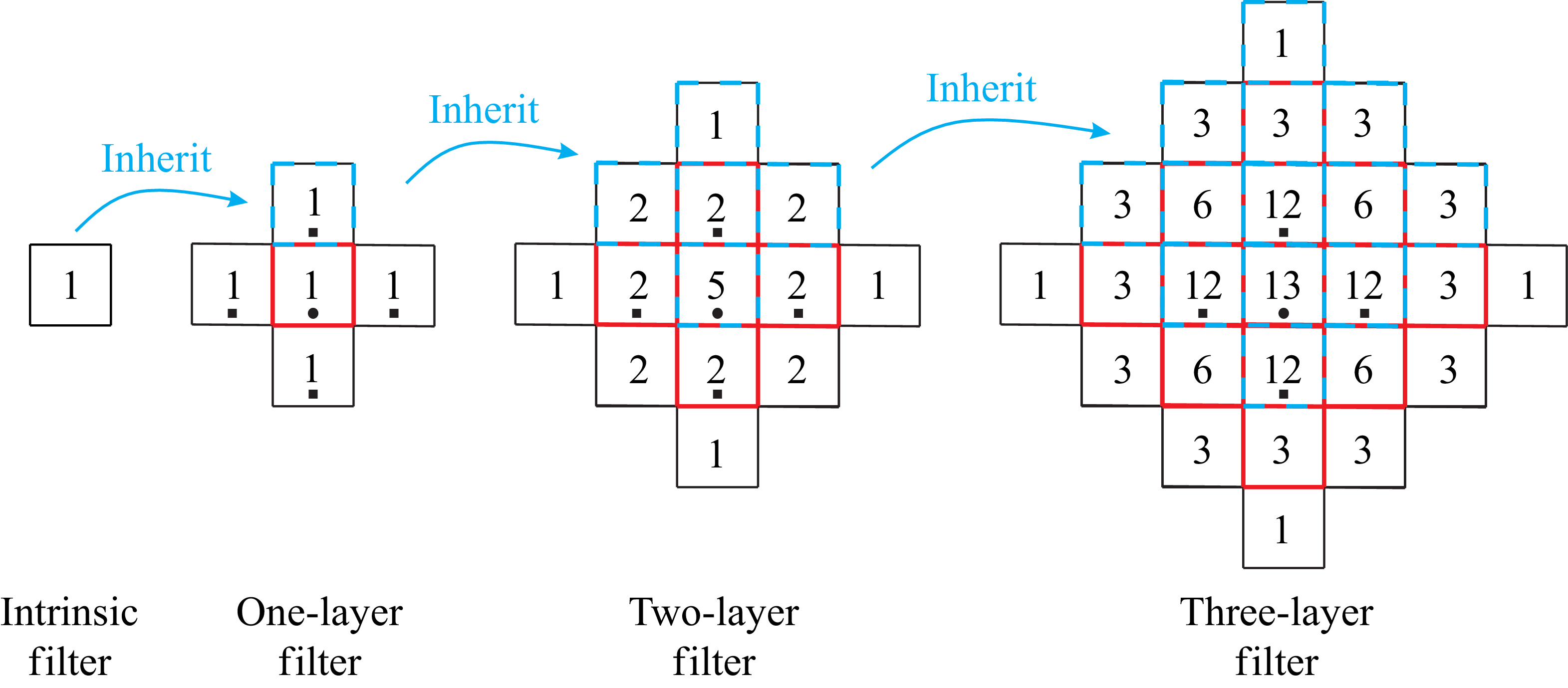
is the weight coefficient of each cell. The distinction between the filters of (2.30) and (3.2) lies in their weighted templates and the coefficients assigned to each cell. The template defined in (2.30) adopts an arbitrary set of grid cells within a neighbourhood around the current grid cell. While useful for mathematical derivations, it is impractical for the actual distributed MPI parallel FVM solver, which struggles to obtain arbitrary multilayer neighbour information. The template of the iterative filter is shown in figure 5, which transmits the multilayer neighbour information by the filter values on the immediate neighbours inherited from the last iterative filter operation. Each new iterative filter performs the weighted average of the last iterative filter information inherited by the current central grid (red dashed box) and that inherited on its immediate neighbours (cyan dashed box). With an increase in the number of iterations, the filter scale will increase layer by layer. For the two-dimensional case, the iterative filtering template is a rhombus-shaped area that expands in four directions (
 $+x,-x,+y,-y$
), while in the three-dimensional case, it expands in six directions (
 $+x,-x,+y,-y,+z,-z$
). However, both filters defined in (2.30) and (3.2) incorporate two types of weight: a density weight reflecting compressibility and a volume weight representing grid scale distribution. In addition, the iterative filter also implicitly incorporates a weight that is inversely proportional to the distance from the central cell. Since there are several
 $M$
-step neighbour routes
 $\sigma (i\ ;\ j_1,j_2,\ldots ,j_M)$
from
 $i$
to
 $j_M$
for a certain cell
 $j_M$
within the template, the weighted summation of (3.2) has multiple terms. After merging, it can be expressed as the following weighted summation:
 \begin{align} &\qquad\qquad \mathcal{F}^{(M)}(Q)_i =\sum _{j \in T(i;M)}\mathcal{F}^\natural (Q)_j\widehat {W}_{i;j}^{(M)}, \end{align}
 \begin{align} & \text{where} \; \widehat {W}_{i;j}^{(M)}= \frac {\overline {\langle \rho \rangle }_j^\natural }{{\overline {\langle \rho _i \rangle }}^{(M)}}\overline {W}_{i;j}^{(M)},\quad \overline {W}_{i;j}^{(M)}=\sum _{\sigma \in \pi (i\rightarrow {j};M)} W_\sigma, \end{align}
Filter templates and cell contribution degree (the number of
 $M$
-step neighbour routes from the central cell to current cell) distribution of iterative filtering in the two-dimensional case.
 $\bullet$
represents the central ith cell and
 $\blacksquare$
represents the immediate neighbours of the ith cell.

where
 $T(i;M)$
represents the
 $M$
-layer filter template and
 $\pi (i\rightarrow {j};\ M)$
represents the set of all
 $M$
-step neighbour routes from
 $i$
to
 $j$
. The numbers marked in figure 5 indicate the number of
 $M$
-step neighbour routes from the central cell to each cell within the template, which is the cardinality of the set
 $\pi (i\rightarrow {j};M)$
, i.e.
 $|\pi (i\rightarrow {j};M)|$
. Since
 $|\pi (i\rightarrow {j};M)|$
is equal to the number repeatedly superimposed of the
 $j$
th cell in the weighted summation of
 $M$
-layer iterative filter of the
 $i$
th cell, we refer to
 $|\pi (i\rightarrow {j};M)|$
as the contribution degree of the
 $j$
th cell to the
 $M$
-layer iterative filter of
 $i$
th cell. For an homogeneous grid,
 $\sum _{\sigma \in \pi (i\rightarrow {j};M)} W_\sigma =|\pi (i\rightarrow {j};M)|/p^M$
, where
 $p$
is the number of immediate neighbours. Then, it can be known that the numbers in figure 5 represent the distance weight. The weight decreases with distance from the central cell for the iterative filter, while the filter in (2.30) maintains constant volume weight on an homogeneous grid.
Figure 6 illustrates the decomposition of Reynolds stress for both the first and fifth iteration of the filter as defined by (3.1). Considering the physical meaning of each residual stress component discussed in § 2.2, as the filtering scale increases, the components
 $\mathcal{A}(\tau _{xx}^C)$
and
 $ \nu _{xx}^C$
– which represent the momentum transfer process caused by turbulent transport at the sub-filter scale – will also increase. Conversely, momentum transfer at the sup-filter scale will decrease, leading to a reduction in
 $ T_{xx}^C$
. As shown in figure 5, as the number of filter iteration layers increases, both
 $\mathcal{A}(\tau _{xx}^C)$
and
 $ v_{xx}^C$
increase, while
 $ T_{xx}^C$
decreases. The results demonstrate that the filter scale increases as the number of iterations rises, causing the stress components of the subgrid to gradually amplify. This confirms the effectiveness of the iterative filter operator defined in (3.1) for stress decomposition analysis within the FVM framework. The situation of large-scale filtering corresponds to the coarse grid solution, where subgrid stress becomes pronounced and the importance of residual stress relation in turbulence modelling will be emphasised.
Decomposition of Reynolds stress in channel flow at
 $Re_{\tau }=180 ,\ Ma_c = 0.1$
with various filter scale size. ,
 $\mathcal{F}(R_{xx}^C)$
; ,
 $\mathcal{A}(\tau _{xx}^C)$
; ,
 $T_{xx}^C$
; ,
 $\nu _{xx}^C$
. The lines with circular symbols represent a five-layer iterative filter, while those without denote a one-layer iterative filter.

The previous discussion on the properties of iterative filtering reveals that as the number of iterative layers increases, the filtering scale expands progressively with a specific weight
 $\overline {W}_{i;j}^{(M)}$
distribution. To examine the actual scale of large-scale flow represented by the iterative filters, we need to calculate the weight distribution. Combining (3.2) and (3.4), the following iterative formula for
 $\overline {W}_{i;j}^{(M)}$
can be obtained:
 \begin{equation} \overline {W}_{i;j}^{(M)}= \sum _{j_{M-1} \in N(j)} \frac {V_j}{\sum _{j \in N(j_{M-1})}V_j}\overline {W}_{i;j_{M-1}}^{(M-1)}. \end{equation}
According to (3.6), we can calculate the distribution of the weight
 $\overline {W}_{i;j}^{(M)}$
of the
 $M$
-layer iterative filter. For the one-layer iterative filter, the number of one-step neighbour routes from the central cell to each cell is one (see the figure 5), and the weight is only affected by the volume distribution
 $\overline {W}_{i;j}^{(1)}=W_{\sigma (i;j)}=V_j/\sum _{j\in N(i)}V_j$
. As long as the volume differences of adjacent cells are not particularly extreme, the influence of each cell on the filtering value in the template cannot be ignored. At this time, the filtering scale is the size of the template. For the
 $M$
-layer iterative filter, since the number of
 $M$
-step neighbour routes of each cell in the template is different, the contribution degree of each cell to the filtering value will show significant differences. Taking the five-layer iterative filter used in the article as an example, figure 7 shows the distribution of the weight
 $\overline {W}_{i;j}^{(M)}$
on the computational grid. It can be seen that the weight far from the central cell decays rapidly, and it is basically insignificant when the central cell expands to the third layer. The non-homogeneity in the y-direction leads to a redistribution of weight, showing symmetry in the x- and z-directions, but a deviation towards the larger volume in the y-direction. Due to the absence of neighbours in the adjacent boundary cell, the expansion of the iterative filtering template will be blocked, thereby affecting the distribution of the weight. Considering the significant region of the weight, the effective filter scale of the five-layer iterative filter in the x- and z-directions is approximately 5–7 times the local cell scale. In the y-direction, it is approximately 3–4 times the local cell scale for the cell close to the boundary, and it is approximately 5–7 times for the cell far from the boundary. In the context of the grid adopted in this paper, the dimensionless scales that relate to local grid scale amplification are
 $\Delta x^+\approx 60{-} 80$
,
 $\Delta z^+\approx 35{-} 50$
and
 $\Delta y^+\approx 0.15{-} 0.2$
adjacent to the boundary, as well as
 $\Delta y^+\approx 20{-} 30$
far from the wall. These scales are almost consistent with the grid filtering scale commonly used in large eddy simulations. The remainder of this paper will focus on analysis using five-layer filtering.
Filter weights of five-layers iterative filtering on the non-homogeneous grid with
 $y_j = \cos (\theta _j)$
normal distribution, where
 $\theta _j = (j-1)\pi /(N-1)$
for
 $j = 1, 2, \ldots , N$
. The normal direction of the grid has been scaled 150 times to be displayed clearly. Left column, the cell far from the boundary; right column, the cell close to the boundary.

The validity of the stress statistical relation described in (2.18) is examined in the context of large-scale filtering. Figures 8 and 9 display the decompositions of the Reynolds normal stress and Reynolds shear stress at various Mach numbers. Figure 10 investigates the decomposition of Reynolds stress at
 $Re_{\tau }=300$
to further verify the residual stress relation formula. In these figures, the hollow circle symbol represents the original Reynolds stress, while the dashed lines illustrate the decomposition of each Reynolds stress component. The solid line reflects the synthesis of these decompositions using (2.18). To clearly highlight the different manifestations of stress distribution in various regions of the boundary layer, logarithmic coordinates are used for the horizontal axis in figures 8, 9 and 10.
Reynolds normal stress decomposition of various channel flows at
 $Re_{\tau }=180$
with different Mach numbers. (a)
 $Ma_c=0.1$
; (b)
 $Ma_c=0.8$
; (c)
 $Ma_c=2.7$
; (d)
 $Ma_c=4.1$
. Five-layer iterative filter: , stress composition
 $\mathcal{A}(\tau _{xx}^C) + T_{xx}^C - \nu _{xx}^C$
; ,
 $\mathcal{A}(\tau _{xx}^C)$
; ,
 $T_{xx}^C$
; ,
 $\nu _{xx}^C$
;
 $\circ$
,
 $\mathcal{F}(R_{xx}^C)$
;
 $\bullet$
,
 $\nu _{xx}^C/\mathcal{F}(R_{xx}^C)$
;
 $\blacksquare$
,
 $\nu _{xx}^C/\mathcal{A}(\tau _{xx}^C)$
. One-layer iterative filter:
 $\boldsymbol{\cdots} \boldsymbol{\cdot}$
,
 $\nu _{xx}^C$
;
 $\square$
,
 $\nu _{xx}^C/\mathcal{A}(\tau _{xx}^C)$
.

Reynolds shear stress decomposition of various channel flows at
 $Re_{\tau }=180$
with different
 $Ma_c$
. (a)
 $Ma_c=0.1$
; (b)
 $Ma_c=0.8$
; (c)
 $Ma_c=2.7$
; (d)
 $Ma_c=4.1$
. Five-layer iterative filter: , stress composition
 $\mathcal{A}(\tau _{xy}^C) + T_{xy}^C - \nu _{xy}^C$
; ,
 $\mathcal{A}(\tau _{xy}^C)$
; ,
 $T_{xy}^C$
; ,
 $\nu _{xy}^C$
;
 $\circ$
,
 $\mathcal{F}(R_{xy}^C)$
;
 $\bullet$
,
 $\nu _{xy}^C/\mathcal{F}(R_{xy}^C)$
;
 $\blacksquare$
,
 $\nu _{xy}^C/\mathcal{A}(\tau _{xy}^C)$
. One-layer iterative filter:
 $\boldsymbol{\cdots} \boldsymbol{\cdot}$
,
 $\nu _{xy}^C$
;
 $\square$
,
 $\nu _{xy}^C/\mathcal{A}(\tau _{xy}^C)$
.


Notably, the solid lines closely overlap with the hollow circle symbols in all of figures 8, 9 and 10, which affirms the accuracy of the residual stress relation presented in (2.18). The normal stress component of the subgrid stress in averaged flow
 $\nu _{xx}^C$
is significant below the logarithmic layer (
 $y^+ \lt 20$
). This is illustrated by the distribution of the filled circle symbol, which represents the ratio of
 $\nu _{xx}^C$
to the Reynolds normal stress
 $\mathcal{F}(R_{xx}^C)$
. As the Mach number increases,
 $\nu _{xx}^C$
in the buffer layer (
 $y^+ \approx 4 {-} 20$
) gradually becomes increasingly prominent in comparison to the subgrid stress
 $\mathcal{A}(\tau _{xx}^C)$
. It can be observed through the variation trend of the filled square symbol, indicating the ratio of
 $\nu _{xx}^C$
to the subgrid stress. Despite being overlooked in existing modelling of compressible wall-bounded turbulence on coarser grids, these findings suggest that
 $\nu _{xx}^C$
may be as crucial as subgrid stress in modelling processes, particularly in compressible flows. Although the ratio of
 $\nu _{xy}^C$
to
 $\mathcal{A}(\tau _{xy}^C)$
increases as
 $Ma_c$
increases,
 $\nu _{xy}^C$
still remains a minor role. In the one-layer iterative filter, as the filter scale decreases, both the sub-filter scale quantities
 $\mathcal{A}(\tau _{xx}^C)$
and
 $\mathcal{A}(\tau _{xy}^C)$
decrease, along with
 $\nu _{xx}^C$
maintaining a proportion with
 $\mathcal{A}(\tau _{xx}^C)$
(as indicated by the ratio
 $\nu _{xx}^C/\mathcal{A}(\tau _{xx}^C)$
, represented by the hollow square symbol). As the
 $Ma_c$
increases, the trend of reduction in
 $\mathcal{A}(\tau _{xx}^C)$
within the one-layer iterative filter is also observed. Although the ratio of
 $\nu _{xy}^C$
to
 $\mathcal{A}(\tau _{xy}^C)$
increases, it is necessary to note that since
 $\mathcal{A}(\tau _{xy}^C)$
is a small quantity, it does not change the value of
 $\nu _{xy}^C$
being close to zero.
The behaviour of each stress component can be illustrated through their physical meanings, as shown in figure 2. First,
 $ T_{\textit{ij}}^C$
(if the value of
 $ij$
is not specified, both
 $xx$
and
 $xy$
are true) represents the momentum transfer associated with turbulence fluctuations that exceed the filter scale. As depicted in figure 11, as the Mach number increases, smaller turbulent structures diminish. A more quantitative analysis is provided through the fluctuation velocity spectrum. The channel flow is homogeneous in the streamwise and spanwise directions, but inhomogeneous in the normal direction. Thus, the one-dimensional signals of the fluctuation velocity along the streamwise direction at different normal positions are extracted to calculate the one-dimensional velocity spectrum through the following definition Pope (Reference Pope2011):
 \begin{equation} E_{uu}(\kappa _1)=\frac {1}{\pi }\int _{-\infty }^\infty R_{uu}(r_1\boldsymbol{e}_1)e^{-i\kappa _1r_1}\,\textrm{d}r_1, \end{equation}
where
 $R_{uu}(r_1\boldsymbol{e}_1)=\langle u^{\prime \prime }(\boldsymbol{x})u^{\prime \prime }(\boldsymbol{x}+r_1\boldsymbol{e}_1) \rangle _E$
is the one-dimensional autocorrelation function of the streamwise fluctuation velocity, and the ensemble average
 $\langle * \rangle _E$
is taken as the average of the spanwise direction and time sequence. Figure 12 shows the one-dimensional energy spectrum distribution of the streamwise fluctuation velocity at different normal positions. To display the proportion of turbulent energy at different scales, the energy spectrum is normalised by the total energy (i.e. the integral of the energy spectrum at each normal position is equal to one). The dash-dotted line in figure 12 indicates the wave number corresponding to the effective filtering scale of the five-layer iterative filtering. As the Mach number increases, the proportion of fluctuation energy contained in small-scale flows above the effective filtering wavenumber gradually decreases, so that the energy contained in the sup-filter scale flows increases. Consequently, the turbulent momentum transfer predominantly occurs within larger-scale structures, leading to an increase in the proportion of
 $ T_{\textit{ij}}^C$
with rising Mach numbers. In contrast, the proportion of
 $ \tau _{\textit{ij}}^C$
, which signifies the turbulence momentum transfer below the filter scale, decreases as the Mach number increases. In the context of
 $ v_{\textit{ij}}^C$
, considering the Taylor expansion of (2.25) with second-order accuracy, the expression for
 $ v_{\textit{ij}}^C$
can be expanded to the following formula:
 \begin{align}&\qquad\qquad\quad \nu _{\textit{ij}}^C = [\ \mathcal{F}(\boldsymbol{r}_i\otimes \boldsymbol{r}_j) - \mathcal{F}(\boldsymbol{r}_i)\otimes \mathcal{F}(\boldsymbol{r}_j)\boldsymbol \ ]{:}\boldsymbol{\nabla }{\langle u_i \rangle }_F\otimes \boldsymbol{\nabla }{\langle u_j \rangle }_F, \end{align}
 \begin{align}& \text{where}\ \ \mathcal{F}(\boldsymbol{r}_i\otimes \boldsymbol{r}_j)=\overline {\boldsymbol{r}_i\otimes \boldsymbol{r}_j}+\overline {\boldsymbol{r}_i\otimes \boldsymbol{r}_j\otimes \boldsymbol{r}_k}\boldsymbol{\cdot }\frac {\boldsymbol{\nabla }_k\rho _c}{\rho _c} , \quad \mathcal{F}(\boldsymbol{r}_i)=\overline {\boldsymbol{r}_i}+\overline {\boldsymbol{r}_i\otimes \boldsymbol{r}_k}\boldsymbol{\cdot }\frac {\boldsymbol{\nabla }_k\rho _c}{\rho _c}, \end{align}
Vortex structures of channel turbulence with different Mach numbers. The vortex identification method is the Q-criterion scaled by
 $u_c^2/\delta$
(
 $Q=0.1$
).

One-dimensional energy spectrum distribution in the normal direction of the fluctuation streamwise velocity. The energy spectrum normalisation ensures that the integral of the energy spectrum at each normal position equals one.

where
 $\boldsymbol{r}_i$
denotes the i-component of radius vector
 $\boldsymbol{r}=\boldsymbol{x}-\boldsymbol{x}_c$
,
 $\boldsymbol{\nabla }_k\rho _c=\partial \rho _c/\partial x_k$
. The term in square brackets contains the geometric quantity associated with the filter scale and the density gradient reflecting the impact of compressibility. It is evident from the equation that
 $ v_{\textit{ij}}^C$
becomes significant in regions with pronounced mean flow gradients, reflecting the momentum transfer generated by the inhomogeneity of the mean flow at the subfilter scale. The flow gradient within the inner boundary layer (comprising the viscous sublayer and the buffer layer) is substantial, indicating the dominant role of
 $ v_{xx}^C$
in this region. The mean velocity in the wall-normal direction inside the boundary layer is small, which contributes to the minor role of
 $ v_{xy}^C$
. As the Mach number increases,
 $ \tau _{\textit{ij}}^C$
decreases due to the diminishment of the small-scale flow fluctuation. Conversely, the increase in the density gradient with increasing compressibility leads to a slight rise in
 $ v_{xx}^C$
. As a result, the proportion of
 $ v_{xx}^C$
relative to
 $ \tau _{xx}^C$
increases with the Mach number.
3.2. Supersonic turbulent boundary layer
In this section, direct numerical simulation of the compressible turbulent boundary layer is adopted to further validate the residual stress relation between the averaged and filtered flow fields established in § 2. The free stream Mach number of the boundary layer flow is 2.0, and the momentum thickness Reynolds number
 $Re_{\theta }$
is 1691 (at the start position of the fully developed zone). The dimensions of the computational domain are illustrated in figure 13. The core region of the supersonic boundary layer is a square box region
 $L_x\times L_y\times L_z=30\delta _0\times 3\delta _0\times 4\delta _0$
, where
 $x$
,
 $y$
and
 $z$
denote to the streamwise, wall-normal and spanwise directions, respectively, and
 $\delta _0$
is the thickness of inlet boundary layer. Downstream of the core region, a
 $10\delta _0$
-length outlet buffer region is added to the end of the computational domain. To ensure the stability of the numerical solution for supersonic flow, a
 $20\delta _0$
-height far-field region with a non-reflective far-field boundary condition is added above the core region, allowing disturbances to decay as propagating to the upper boundary of the computation domain. The wall condition for the boundary layer is set to an adiabatic no-slip wall, while the downstream of the core region adopts a slip wall to buffer the flow to the no-reflective outlet. The periodic boundary condition is applied in the spanwise direction. To accelerate the development of turbulence, a synthetic turbulence method that accounts for the turbulence structures of the inner and outer layers is employed to the inlet. This method was developed by Sandham, Yao & Lawal (Reference Sandham, Yao and Lawal2003) and implemented by Pirozzoli, Bernardini & Grasso (Reference Pirozzoli, Bernardini and Grasso2008) in the numerical simulation of supersonic boundary layer flows. Further details regarding the specific implementation of synthetic turbulence can be found from Pirozzoli et al. (Reference Pirozzoli, Bernardini and Grasso2008).
Computational domain and boundary condition of supersonic turbulent boundary layer.

The grid point number of the core region in the streamwise, wall-normal and spanwise directions is
 $620\times 180\times 128$
. The grid in the streamwise direction is uniformly distributed with a dimensionless grid size
 $\Delta x^+ = 11.5$
scaled by the viscous scale at the start position of fully developed turbulence. The spanwise grid is also uniformly distributed with a spacing
 $\Delta z^+ = 7.4$
. The first layer spacing at the wall surface is
 $\Delta y_w^+ = 0.8$
. The wall-normal grid distribution refers to Pirozzoli et al. (Reference Pirozzoli, Bernardini and Grasso2008) that was stretched according to a hyperbolic sine function
 $\sin h(b\theta )/\sin h(b), \ \theta =(i-1)/(N-1), \ i=1,2,\ldots ,N$
up to the boundary layer edge and distributed the gird point with a geometric progression to the upper edge of the core region. Additionally, a number of 20 points are allocated for both the streamwise direction of the outlet region (
 $x\gt 30\delta _0$
) and the wall-normal direction of the far-field region (
 $y\gt 3\delta _0$
) to buffer the flow to the boundary of the computational domain. Figure 14 illustrates the fluctuation velocity field at the cross-section of
 $y^+=24$
, which corresponds to the upper edge of the buffer region of the boundary layer. It can be seen that the synthetic turbulence at the inlet develops over a certain distance and ultimately evolves into regular streak structures near the wall region. As the flow transitions to developed turbulence, wall friction coefficient increases, reaching a maximum value near
 $x=22\delta _0$
, which indicates the start position of fully developed turbulence.
Streak structures of fluctuation velocity
 $u^{\prime \prime }/u_e$
at
 $y^+=24$
and friction coefficient on the wall.

The numerical results of the supersonic boundary layer have been validated against the DNS data from Guarini et al. (Reference Guarini, Moser, Shariff and Wray2000) and Pirozzoli et al. (Reference Pirozzoli, Bernardini and Grasso2008). The boundary layer flow parameters adopted by Pirozzoli et al. (Reference Pirozzoli, Bernardini and Grasso2008) are
 $Ma = 2.0$
and
 $Re_\theta = 1350$
, and the parameters of Guarini et al. (Reference Guarini, Moser, Shariff and Wray2000) are
 $Ma = 2.5$
and
 $Re_\theta = 1577$
. To ensure the flow parameters are as consistent as possible with the reference data, we investigate the results at the starting position of the fully developed turbulence zone, located at
 $x = 22\delta _0$
, with
 $Ma = 2.0$
and
 $Re_\theta = 1691$
. The friction Reynolds number here is
 $Re_\tau =314$
. Figure 15 presents a comparison of the mean velocity profile, the root mean square (r.m.s.) of the fluctuation velocity and the Reynolds shear stress. The compressible boundary layer velocity is transformed using the Van Driest transformation to align with the scaling law applicable to incompressible flow. Furthermore, the r.m.s.s of the fluctuation velocity and Reynolds shear stress are also scaled by
 $\rho /\rho _w$
to be consistent with the reference data,
 \begin{equation} u_{VD} = \int _0^u\sqrt {\frac {\rho }{\rho _w}}\,\textrm{d}u. \end{equation}
The results indicate that the mean streamwise velocity profile adheres to the linear-law
 $u^+=y^+$
in the viscous sub-layer as well as the log-law
 $u^+=1/\kappa \ \ln y^++C, \ C=4.7$
in the logarithmic layer, and aligns closely with the DNS results of Guarini et al. (Reference Guarini, Moser, Shariff and Wray2000) and Pirozzoli et al. (Reference Pirozzoli, Bernardini and Grasso2008). Additionally, the second-order statistics, including the r.m.s. of each velocity component and Reynolds shear stress, show good agreement with the reference data, confirming the validity of the DNS calculations presented in this paper.
Statistics quantities at
 $x=22\delta _0$
with
 $Re_{\theta }=1691$
compared with Pirozzoli et al.(
 $Re_\theta = 1350$
) and Guarini et al.(
 $Re_\theta = 1577$
). (a) Streamwise velocity. , present
 $u_{VD}^+$
; ,
 $u^+=1/0.41\ lny^++4.7$
and
 $u^+=y^+$
;
 $\circ$
, Guarini et al.;
 $\triangle$
, Pirozzoli et al. (b) , r.m.s. of streamwise velocity; , r.m.s. of spanwise velocity; , r.m.s. of wall-normal velocity; , Reynolds shear stress.

The flow of the boundary layer is non-homogeneous along the stream direction. To further validate the generality of the residual stress relation proposed in § 2.2, stress decomposition is investigated at different streamwise positions. Figure 16 examines two distinct streamwise positions: a turbulent developing region and a fully developed region for stress decomposition. At position
 $x = 5\delta _0$
, there is a non-attenuation phenomenon of the resolved normal stress (
 $T_{\textit{ij}}^C$
) in the outer logarithmic region (
 $y^+ \gt 30$
) of the boundary layer, which is influenced by the synthetic turbulence disturbance at the inlet. As the flow progresses downstream and reaches the fully developed status (
 $x = 22\delta _0$
), the impact of the inlet disturbance gradually diminishes, resulting in a canonical decay of the normal stress in the outer logarithmic region of the boundary layer. Additionally, the peak values of normal stress and shear stress in the fully developed zone are slightly higher than those observed in the developing zone. Under the influence of these phenomena, the stress decomposition formula can effectively establish the relation of the residual stress between the averaged and filtered flow. The composition of each stress component accurately reproduces the distribution characteristics of the Reynolds stress at both locations.
Streamwise normal stress (upper half plane) and shear stress (lower half plane) decomposition at two streamwise positions (scaled by
 $u_\tau ^2$
). The number of iterative filtering is five. , stress composition
 $\mathcal{A}(\tau _{\textit{ij}}^C) + T_{\textit{ij}}^C - \nu _{\textit{ij}}^C$
; ,
 $\mathcal{A}(\tau _{\textit{ij}}^C)$
; ,
 $T_{\textit{ij}}^C$
; ,
 $\nu _{\textit{ij}}^C$
;
 $\circ$
,
 $\mathcal{F}(R_{\textit{ij}}^C)$
. (a) Developing position(
 $5\delta _0$
); (b) developed position(
 $22\delta _0$
).

The relation of turbulent heat flux between the averaged and filtered flow fields presented in § 2.2 has also been verified. Similar to the investigation of residual stress, the turbulent heat flux at two specific streamwise positions is considered for decomposition by using (2.21). As shown in figure 17, the distribution characteristics of turbulent heat flux closely resemble those of Reynolds stress. Consistent with the findings regarding residual stress, the resolved turbulent heat flux increases as turbulence develops downstream, while the heat flux associated with the subgrid-scale decreases correspondingly. The composition of each component of the turbulent heat flux can effectively recover the heat flux at each streamwise position within the boundary layer, thereby confirming the validity of the heat flux relation expressed in (2.21).
Heat flux decomposition at two streamwise positions (scaled by
 $u_\tau ^3$
). The number of iterative filtering is five. , heat flux composition
 $\mathcal{A}(q_{sgs,x}) + S_x - \omega _x$
; ,
 $\mathcal{A}(q_{sgs,x})$
; ,
 $S_x$
; ,
 $\omega _x$
;
 $\circ$
,
 $\mathcal{F}(q_{x}^t)$
. (a) Developing position(
 $5\delta _0$
); (b) developed position(
 $22\delta _0$
).

The behaviour of the decomposition terms of Reynolds stress and turbulent heat flow on the flat boundary layer can be demonstrated through the multi-scale physical understanding of turbulence. First, in the context of momentum and heat transfer resulting from the transport of the sub-filter scale turbulence, the flow near the inlet contains artificial small-scale disturbances, leading to large values of
 $ \tau _{\textit{ij}}^C$
(if the value of
 $ij$
is not specified, both
 $xx$
and
 $xy$
are true) and
 $ q_{sgs,x}$
at the position
 $ x = 5\delta _0$
. As the flow develops downstream, it gradually transitions into a natural turbulent state and the artificial disturbance is attenuated, resulting in a decrease in
 $ \tau _{\textit{ij}}^C$
and
 $ q_{sgs,x}$
at the fully developed turbulence location of
 $ x = 22\delta _0$
. During this process, the turbulent energy cascade is gradually established, with more energy being transferred from the main flow to the large-scale flow through shear effects. Consequently,
 $ T_{\textit{ij}}^C$
and
 $ S_x$
both increase within the buffer layer at the position
 $ x = 22\delta _0$
. Shear effects are most pronounced in the buffer layer, where the large-scale turbulent energy transferred from the main flow is also the most significant. As the shear effect diminishes when moving towards the outer layer, the transferred large-scale turbulent energy gradually decreases. This physical process is also reflected in the behaviour of
 $ T_{\textit{ij}}^C$
and
 $ S_x$
: from
 $ x = 5\delta _0$
to
 $ x = 20\delta _0$
, the distribution of
 $ T_{\textit{ij}}^C$
and
 $ S_x$
in the outer layer of the boundary layer changes from an abnormal rise or plateau phenomena caused by artificial disturbances to a gradually decreasing distribution that is dominated by real physics. The momentum and heat transfer induced by the inhomogeneity of the mean flow below the filter scale, characterised by
 $ \nu _{\textit{ij}}^C$
and
 $ \omega _x$
, is also evident in the decomposition results. This is manifested in a significant distribution of
 $ \nu _{xx}^C$
in the inner boundary layer arising from a strong mean flow gradient and a near-zero
 $ \nu _{xy}^C$
due to a small mean normal velocity in the boundary layer.
4. Conclusion
Numerical investigations in compressible channel flow reveal that the Reynolds stress defined by Favre and Reynolds averages observably differs at higher Mach numbers, rendering the existing residual stress relations ineffective. To address this, a new statistical relation for residual stress in compressible flows has been developed through theoretical research and numerical verification. A novel pair of averaging/filtering operators with commutative properties is defined to enable the derivation of the relation between Reynolds stress and SGS stress without any assumptions. Using the same pair of averaging/filtering operators, the noteworthy decomposition of turbulent heat flux in compressible flow is also rigorously derived. Various filtering operators have been formulated within the FVM framework, commonly used in engineering turbulence simulations, to enhance applicability in the aerospace engineering community. Numerical experiments involving compressible channel flow at various Ma and compressible boundary layer flow validate the accuracy of the residual stress relation and the effectiveness of the filter operator. Further physical analysis indicates that the residual stress relation formula decomposes the momentum transfer generated by turbulent transport into three momentum transfer component processes caused by the sup-filter scale turbulent transport, sub-filter scale turbulent transport and the inhomogeneous of mean flow, which provides an analytical tool for the multiscale analysis of turbulence. In addition, the residual stress relation formula establishes the connection of modelled stress between RANS and LES, which provides a new way to solve the problem of modelled stress deficiency during the RANS/LES region conversion of the hybrid RANS/LES method.
Acknowledgements
The computations were conducted in the Computing Center in Xi’an. The authors thankfully acknowledge this institution.
Funding
The research was supported by the National Natural Science Foundation of China (No. U2141254 and No. U23B6009).
Declaration of interests
The authors report no conflict of interest.
Data availability statement.
The data that support the findings of this study are available from the corresponding author upon reasonable request.
Appendix A.
In this appendix, we present an application of the proposed residual stress relation formula to the hybrid RANS/LES method, demonstrating its potential contributions to turbulence modelling. Under the framework of the detached eddy simulation (DES), one of the most widely used hybrid approaches (Spalart Reference Spalart2009), a new RANS / LES hybrid strategy is proposed that incorporates the residual stress relation. The key to turbulence modelling lies in addressing the residual stress, which is an unclosed term in the averaged or filtered Navier–Stokes equations. To achieve closure of them, the transport equation for the residual stress
 $R_{\textit{ij}}$
with fewer physical assumptions is adopted,
 \begin{equation} \frac {\partial }{\partial t}(\rho R_{\textit{ij}})+\frac {\partial }{\partial x_k}(\rho U_kR_{\textit{ij}})=\rho P_{\textit{ij}}-\rho \epsilon _{\textit{ij}} + \rho \varPi _{\textit{ij}}+\rho D_{\textit{ij}}, \end{equation}
where
 $U_k$
denotes the averaged or filtered velocity. Here,
 $P_{\textit{ij}}$
,
 $\epsilon _{\textit{ij}}$
,
 $\varPi _{\textit{ij}}$
and
 $D_{\textit{ij}}$
are the production term, the dissipation term, the redistribution term and the diffusion term of residual stress, respectively. The terms on the right-hand side of (A1) are all unclosed except for the production terms, and the detailed closure calculation can be found from Li et al. (Reference Li, Chen, Wang and Liu2022) and Cécora et al. (Reference Cécora, Radespiel, Eisfeld and Probst2015). In the context of the DES-class method, the dissipation term
 $\epsilon _{\textit{ij}}$
is modelled using the following equation, which is discussed in detail by Wang, Li & Liu (Reference Wang, Li and Liu2021):
 \begin{equation} \epsilon _{\textit{ij}} = \dfrac {2}{3} \frac {k^{\frac{3}{2}}}{l_{\textit{DES}}}\delta _{\textit{ij}}= \begin{cases} \dfrac {2}{3} \dfrac {k^{\frac {3}{2}}}{l_{\textit{LES}}}\delta _{\textit{ij}}=\dfrac {2}{3} \dfrac {k^{\frac {3}{2}}}{C_{\textit{DES}}\varDelta }\delta _{\textit{ij}} , \ \ C_{\textit{DES}}=C_s C_k \quad \text{LES region}, \\ \\ \dfrac {2}{3} \dfrac {k^{\frac {3}{2}}}{l_{\textit{RANS}}}\delta _{\textit{ij}}=\dfrac {2}{3} \dfrac {k^{\frac {3}{2}}}{\big(1/C_\mu ^{1/n}C_l\big)l}\delta _{\textit{ij}} , \ \ l=C_lk^{\frac {m}{n}+\frac {3}{2}}\phi ^{-\frac {1}{n}} \quad \text{RANS region}, \end{cases} \end{equation}
where
 $l_{\textit{DES}}=f (l_{\textit{RANS}}\rm{,\ } l_{\textit{LES}} )$
,
 $k$
is the turbulent kinetic energy defined by half-trace of residual stress
 $k=({1}/{2})R_{ii}$
,
 $\varDelta$
is the grid scale, calculated by
 $\varDelta =\max(\Delta x,\Delta y,\Delta z)$
,
 $\phi$
in (A2) represents the turbulence scale variable, which can be taken as the dissipation rate of turbulent kinetic energy
 $\varepsilon$
or specific dissipation rate
 $\omega$
, and the parameter value in the equation can be found from Wang et al. (Reference Wang, Li and Liu2021). The factor 2/3 in (A2) is to ensure that the result of the half-trace of Reynolds stress dissipation rate
 $\epsilon _{\textit{ij}}$
is equal to the turbulent kinetic energy dissipation rate
 $\varepsilon$
, to guarantee the compatibility of the definitions of the two dissipation rates. The mixing length function
 $f$
is a switching function that facilitates the transition between RANS and LES dissipation modes in a specific region. The design of
 $f$
is crucial for the DES method. The original mixing length function was proposed by Spalart (Reference Spalart1997), employing a minimum function of the RANS length scale and the LES length scale to enable RANS in the near-wall region and LES in regions farther from the wall,
 \begin{equation} l_{\textit{DES}}=\min\left (l_{\textit{RANS}}\rm{,\ } l_{\textit{LES}}\right ). \end{equation}
This mixing length function may activate the LES within the boundary layer prematurely, even when the local grid scale does not meet the requirements for LES resolution. This can lead to a log-layer mismatch (LLM) problem in the boundary layer. To address this issue, Spalart and Shur introduced a delayed DES (DDES, Spalart et al. Reference Spalart, Deck, Shur, Squires and Strelets2006), as well as an improved version of DDES (IDDES, Shur et al. Reference Shur, Spalart, Strelets and Travin2008) by preventing LES intrusion with a shielding function in the boundary layer. However, this approach has some drawbacks. First, the shielding function is artificial, relying on empirical coefficients, which limits its universality. Second, it forces DES to adopt the RANS in most region of the boundary layer, thereby diminishing the capacity for turbulent resolution, even when the grid scale is sufficiently small to support LES resolution.
The residual stress relation formula proposed in this paper establishes a relationship between the Reynolds stress and the subgrid-scale stress. This offers an alternative solution to the LLM problem without the need for an artificial shielding function. The LLM issue in the DES method arises from modelled stress deficiency caused by LES intrusion on a coarse grid. By means of the residual stress relation (2.18), the deficiency stress can be statistically obtained from the filtered flow field and offset to the modelled stress. The specific calculation formula is shown as follows:
 \begin{equation} M_{\textit{ij}}= \begin{cases} R_{\textit{ij}}^{\textit{mod}}, \ \ \ \ \ \ \ \ \ \ \ \ \ \ \ \ \ \ \ \ \ \ \ \ \ \ \ \ \ \ \ \ \ \ \ \ \ \ \ \ \ \ \ \ \ \ \ \ \ \ \ \ \ \ \ \ \ \ \ \ \ \ \ \ l_{\textit{RANS}}\lt C_{\textit{DES}}\varDelta, \\ \\ \tau _{\textit{ij}}^{\textit{mod}} + g\big(\frac {k_{\textit{res}}}{k_{tot}}\big)\big(\mathcal{A}\big(\tau _{\textit{ij}}^C\big) + T_{\textit{ij}}^C - \nu _{\textit{ij}}^C-\tau _{\textit{ij}}^{\textit{mod}}\big), \ \ \ l_{\textit{RANS}} \geqslant C_{\textit{DES}}\varDelta, \end{cases} \end{equation}
where
 $\ g({k_{\textit{res}}}/{k_{tot}})=- ({1}/{2})(\tanh(100({k_{\textit{res}}}/{k_{tot}}-\eta ) )-1)$
.
In (A4),
 $R_{\textit{ij}}^{\textit{mod}}$
represents the modelled Reynolds stress calculated by (A1) with dissipation term of
 $k^{{3}/{2}}\delta _{\textit{ij}}/l_{\textit{RANS}}$
, corresponding to the RANS region. Conversely,
 $\tau _{\textit{ij}}^{\textit{mod}}$
represents the modelled subgrid-scale stress computed using dissipation term of
 $k^{(3/2)}\delta _{\textit{ij}}/l_{\textit{LES}}$
, corresponding to the LES region. The function
 $g$
is the offset control function, where
 $k_{\textit{res}}$
is the resolution turbulent kinetic energy and
 $k_{tot}$
is the total turbulent kinetic energy, calculated by the half-trace of (2.18). The parameter
 $\eta$
serves as the resolution evaluation criterion, where a criterion for fine LES that the resolution turbulent kinetic energy must account for more than 85 % (Pope Reference Pope2011). When the LES resolution is insufficient (
 $k_{\textit{res}}/k_{tot}\lt 0.85$
),
 $g$
tends to 1, and the turbulent modelled stress
 $M_{\textit{ij}}$
will be offset to Reynolds stress
 $\mathcal{F}(R_{\textit{ij}}^C)$
. In contrast, if LES is fully resolved,
 $g$
tends to 0, and the modelled stress
 $M_{\textit{ij}}$
remains as the subgrid-scale stress
 $\tau _{\textit{ij}}^{\textit{mod}}$
on the grid cell,
 \begin{equation} k_{tot}=\frac {1}{2}\mathcal{F}\big(R_{ii}^C\big)=\frac {1}{2}\big(\mathcal{A}\big(\tau _{ii}^C\big) + T_{ii}^C - \nu _{ii}^C\big) , \quad k_{\textit{res}} = \frac {1}{2}T_{ii}^C. \end{equation}
The new DES method, referred to as offset DES (ODES), addresses the LLM problem through stress offset in regions where the LES resolution is inadequate. The ODES method is numerically validated through the compressible boundary layer case presented in § 3.2, with comparisons against the DNS, DES and IDDES methods. DES, IDDES and ODES are performed using the same setting as DNS, but they are computed on a coarser grid with dimensions of streamwise
 $\times$
spanwise
 $\times$
normal = 210
 $\times$
64
 $\times$
180. As illustrated in figure 18, the DES method exhibits a significant LLM problem in the logarithmic layer. In contrast, the velocity profiles predicted by ODES and IDDES methods are in good agreement with that obtained by DNS in the logarithmic region. The influence of
 $\eta$
values on the results is also investigated. When the
 $\eta$
value is small, the stress compensation is weak and the LLM issue cannot be fully eliminated (as shown in figure 18 with
 $\eta = 0.7$
). When the
 $\eta$
value is large, the stress compensation effect is strong. Although it can effectively eliminate the LLM issue, excessive stress compensation will also cause the turbulent fine structures to be dissipated, reducing the turbulent resolution capacity of the ODES method (as shown in figure 19 with
 $\eta = 0.9$
). It is recommended to set
 $\eta = 0.85$
, which is also the thumb criterion for fine LES resolution.
Velocity profiles obtained by various turbulence modelling methods. , ODES (
 $\eta =0.7$
); with symbols, ODES (
 $\eta =0.85$
); , ODES (
 $\eta =0.9$
); , DES; , IDDES; ,
 $u^+=y^+$
and
 $u^+=1/0.41\ lny^++4.7$
;
 $\circ$
, DNS.

Streak structures of fluctuation velocity
 $u^{\prime \prime }/u_e$
at
 $y^+=24$
obtained by various turbulence modelling methods.

While the IDDES method also avoids the LLM problem, its shielding function leads to the RANS solution across most regions within the boundary layer, which limits the resolution of turbulent structures achieved by IDDES. Figure 19 demonstrates that IDDES performs less effectively than ODES in resolving the streak structures within the boundary layer. ODES successfully mitigates the LLM issue while preserving the capability to finely resolve the turbulent structures.