


1. Introduction
This paper compares various redistribution policies under the same transfer budget. This is motivated by the “autopilot” feature of many U.S. income-support programs, that are set by law rather than annual congressional appropriations. In practice, the budget size of each program is automatically determined by eligibility criteria and the number of recipients. A longstanding controversy thereon is whether programs should be universal or conditional on economic status, while universality and conditionality generally imply different program sizes. Such differences confound policy comparisons: the economic impacts of policy reflect not only policy design but also the total amount of transfer expenditure. This naturally raises the question of how different policy designs affect the economy when they start from the same level of transfer spending. In this paper, we isolate the role of policy design by comparing programs under an identical level of initial transfer expenditure.
We compare (i) a nonlinear tax-and-transfer program, (ii) a negative income tax (NIT), and (iii) a universal basic income (UBI), under an identical initial fiscal commitment. First, the nonlinear tax-and-transfer program reflects the progressive U.S. income tax schedule. We capture both taxes and transfers by employing the net tax function from Heathcote et al. (Reference Heathcote, Storesletten and Violante2017). Second, NIT represents the conditional income-support programs. Only the low-income households that earn less than the income threshold receive transfer, which phases out linearly as income rises. The high-income households that earn more than the threshold pay linear taxes for their excessive incomes. Lastly, UBI is a universal program. Everyone faces the same tax rate, and everyone receives the same lump-sum transfer.
We evaluate these programs in an incomplete markets environment à la Aiyagari (Aiyagari, Reference Aiyagari1994), with the baseline economy calibrated to approximate the U.S. income distribution. For the identical level of initial transfer expenditures across policies, we take the Ramsey-style approach. We compute the degree of tax progressivity in the nonlinear tax-and-transfer program and marginal tax rate (MTR) of NIT required to finance the optimal UBI in Chang et al. (Reference Chang, Han and Kim2024). UBI is often considered expensive (Van Parijs et al. Reference Van Parijs, Jacquet and Salinas2000), because it guarantees an unconditional lump-sum transfer to the superrich as well as the poor. As an alternative conditional instrument, NIT from Friedman et al. (Reference Friedman, Friedman and Gardner1962) is known for its simplicity, and it has played a key role in shaping modern welfare research (Moffitt, Reference Moffitt2003). However, the MTR needed to finance the minimum income under NIT remains unclear (Lopez-Daneri, Reference Lopez-Daneri2016), while NIT is considered cheaper than UBI (Chang et al. Reference Chang, Han and Kim2024). According to the study of Chang et al. (Reference Chang, Han and Kim2024), NIT can replicate the ex post income distribution of UBI with smaller government budget. In our framework, where policies have the same government budget initially, the MTR of NIT is significantly higher than that of Chang et al. (Reference Chang, Han and Kim2024), and tax progressivity more than doubles that of Heathcote et al. (Reference Heathcote, Storesletten and Violante2017). These substantial increases in taxes to finance UBI can lead to reductions in labor, capital, and welfare (see Guner et al. Reference Guner, Kaygusuz and Ventura2023; Jaimovich et al. Reference Jaimovich, Saporta-Eksten, Setty and Yedid-Levi2026), consistent with our results. Guner et al. (Reference Guner, Kaygusuz and Ventura2023) also highlight that running these programs can bring large administrative costs, which is further studied by Guimarães and Lourenço (Reference Guimarães and Lourenço2024). We abstract from such imperfections of welfare programs in order to focus on how policy designs affect the economy.
One of the main findings of this study is that the nonlinear tax-and-transfer program distorts the macroeconomy more than the linear policies (NIT and UBI) do, when the initial transfer expenditures are identical across policies. First, while balancing the government budget in each policy, all three policies decrease labor supply and savings. Consequently, the aggregate output in the new steady state relative to the laissez-faire economy drops by 6.1% under UBI, 20% under NIT, and 27.4% under the nonlinear tax-and-transfer program. This arises from high tax rates under the nonlinear tax-and-transfer program and NIT needed to finance the optimal UBI. Also, all three policies experience aggregate welfare gain in the short run, but the long-run welfare is positive only under UBI. Moreover, a broader range of households are better off under UBI, whereas the nonlinear tax-and-transfer program and NIT have more polarized welfare gains among households. Second, we consider an alternative experiment in which the policy rules are held fixed over time. In this case, the nonlinear tax-and-transfer program brings a conditional Pareto improvement at the cost of an 8.72% tax deficit relative to GDP. Also, NIT has the largest distortion in the economy among three policies, leading to 33% decrease in aggregate output and 13.3% tax deficit, relative to GDP. The tax deficits arise because redistribution shrinks the tax base while the policy rules remain unchanged. Therefore, these welfare gains are not resource-feasible without an additional source of financing.
Our results are consistent with the “leaky bucket” theory of Okun (Okun, Reference Okun2015). All three policies in our model shrink the tax base, as they disincentivize labor and savings. With shrinking tax base, we balance the government budget by adjusting transfer rules over time so that policies are implemented without tax deficits. In contrast, policies generate fiscal deficits if the transfer rules are held fixed over time, and we also track this tax deficit associated with each policy. This experiment is motivated by the Congressional Research Service report, which shows that the federal deficit was 5.9% of GDP in 2023 (Austin, Reference Austin2023).Footnote 1 Although tracking tax deficit brings imbalance in the government budget in our model due to redistributive distortions (shrinkage in the tax base), our approach allows for isolating the general equilibrium responses and measuring the pure redistributive effects. Despite this imbalance, the model remains internally consistent and allows us to quantify the effects of redistribution under nonclearing markets, in line with the disequilibrium literature (see Barro and Grossman Reference Barro and Grossman1971 and Mankiw Reference Mankiw2006).
This paper is closely related to the literature on the comparisons of UBI and NIT. Both policies may be perceived similarly by taxpayers, or that the difference is a matter of framing (Harvey, Reference Harvey2006; Mankiw, Reference Mankiw2021). Within this debate, Chang et al. (Reference Chang, Han and Kim2024) formalize conditions under which NIT can replicate the allocation under UBI with a smaller government budget. Holding the same MTRs, their quantitative exercise implies a tax-to-GDP ratio of 15.4% under UBI versus 3.8% under NIT for identical ex post distributions, highlighting a potential efficiency advantage of conditional design. Despite its efficiency advantages, NIT has not been widely adopted in practice, and Friedman (Reference Friedman1968) argues that it may generate upward political pressure on the threshold income. In our model, this upward political pressure can be relieved to some extent under the nonlinear tax-and-transfer program because the tax progressivity moves the break-even income higher, which we show later in Proposition1. In Chang et al. (Reference Chang, Han and Kim2024), although the tax rates are set identical and thus UBI and NIT have the same ex post distributions, the total amount of transfer expenditures differ. Also, they mention that their analysis is restricted to a linear tax schedule. We contribute to this line of research by implementing nonlinearity with Ramsey approach (Ramsey, Reference Ramsey1927), in which financing instruments are endogenously determined: we compute the tax progressivity and NIT tax rate required to finance the optimal UBI benchmark from Chang et al. (Reference Chang, Han and Kim2024). Our framework allows for implementing identical total amount of transfer expenditures across policies at the initial period. We thereby isolate how differences in policy design, rather than program size, transform a common fiscal commitment into distinct macroeconomic and distributional consequences.
Another line of literature studying UBI focuses on labor market. For instance, Fabre et al. (Reference Fabre, Pallage and Zimmermann2014) and Rauh and Santos (Reference Rauh and Santos2022) analyze environments with idiosyncratic employment risk, vacancy creation, wage determination, and welfare within labor matching frameworks, while Conesa et al. (Reference Conesa, Li and Li2023), Daruich and Fernández (Reference Daruich and Fernández2024), Luduvice (Reference Luduvice2024), and Ferreira et al. (Reference Ferreira, Peruffo and Valério2025) incorporate endogenous human capital accumulation. In contrast, we abstract from labor market frictions and human capital accumulation, and instead model labor supply decisions directly at the household level in order to isolate the policy effects on the intensive margin.
The rest of the paper is constructed as follows. Section 2 presents the model and calibration. Section 3 reports the transition paths of macroeconomy and welfare, steady state results, and household value gains. Section 4 studies robustness to labor supply elasticities and targeted average working hours. Section 5 exercises the fixed transfer rule case which causes a tax deficit, and Section 6 concludes.
2. Methodology
In this Section, we explain the model economy. In Section 2.1 we clarify the mechanism of this study in a heterogeneous agent economy based on Aiyagari (Reference Aiyagari1994) and Chang et al. (Reference Chang, Han and Kim2024). In Section 2.2 we provide analytical analysis of the government budget that is initially identical across policies, then explain the calibration process to match to the U.S. income distribution in Section 2.3.
2.1 Model
2.1.1 Households
Similarly to Chang et al. (Reference Chang, Han and Kim2024), we consider a closed economy with a continuum of infinitely lived households who face uninsurable and idiosyncratic income shocks in the incomplete markets environment (Aiyagari, Reference Aiyagari1994). A distinction in our model setup from Chang et al. (Reference Chang, Han and Kim2024) is that the households face different disposable incomes under each policy. This arises from comparing the mechanisms of tax-and-transfer policies under the same amount of initial transfer expenditures, explained in 2.1.3.
At time
 $t$
, households earn income
 $y_{t}$
from both labor and assets (
 $y_{t}=w_{t}x_{t}h_{t}+r_{t}a_{t}$
), where
 $w_{t},x_{t},h_{t},r_{t},a_{t}$
denote wage rate, productivity, working hours, interest rate, and asset holdings, respectively. The uninsurable productivity shock follows an AR(1) process:
 $\ln x' = \rho \ln x+ \epsilon _{x}$
, where
 $\epsilon _{x} \sim N(0,\sigma _{x}^{2})$
. This process induces a transition probability
 $\pi (x'|x)$
, which denotes the conditional probability of next-period productivity
 $x'$
given current productivity
 $x$
. The households take the factor prices
 $w_{t},r_{t}$
as given and, for each state
 $(a_{t},x_{t})$
, choose consumption
 $c_{t}$
, next-period asset holdings
 $a_{t+1}$
, and labor supply
 $h_{t}$
to maximize their expected lifetime utility, subject to the household budget constraint. The joint distribution of asset and productivity is denoted by
 $\Phi _{t}(a,x)$
, and the households face a borrowing constraint (
 $a_{t+1} \geq 0$
), accumulating precautionary savings to insure against future income shocks. This dynamic optimization problem can be formulated recursively in the Bellman equation and be solved using the value function iteration method:
 \begin{align} \begin{split} V(a,x)&=\max \{ u(c,h)+ \beta \mathbb{E}[V(a',x')|x] \}, \\ \text{ s.t. } c+a'&=a+\text{disposable income}. \end{split} \end{align}
The value function after redistribution is compared with its laissez-faire counterpart, and we measure household value gain with this difference (see Figures 3 and A.7). Utility function
 $u(c,h)$
is additive separable with a standard risk-averse CRRA form including the disutility of labor
 $B$
and labor supply elasticity
 $\gamma$
as:
 $u(c,h)=\ln c - B\frac {h^{1+1/\gamma }}{1+1/\gamma }$
.
2.1.2 Firms
The production function
 $F(L_{t},K_{t})$
of a representative firm follows the Cobb–Douglas form:
 $Y_{t}=F(L_{t},K_{t})=L_{t}^{\alpha }K_{t}^{1-\alpha }$
, where
 $\alpha$
,
 $L$
and
 $K$
denote labor share, aggregate effective labor and aggregate capital, respectively at time
 $t$
. In each period, capital depreciates at the rate of
 $\delta$
, and the factor prices are determined from the firm’s profit maximization problem as:
 $w_{t}=\alpha (K_{t}/L_{t})^{1-\alpha }$
, and
 $r_{t}=(1-\alpha )(K_{t}/L_{t})^{-\alpha }-\delta$
.
2.1.3 Government
The government insures households against idiosyncratic shocks through tax-and-transfer policies. The government budget is balanced within each policy, and initial budgets are set to be identical across policies. Below we explain the following three policies: (i) a nonlinear tax-and-transfer program, (ii) an NIT, and (iii) a UBI.
Nonlinear tax-and-transfer program.
We employ the well-known HSV net tax function from Heathcote et al. (Reference Heathcote, Storesletten and Violante2017), so that our results are directly comparable with the tax literature.Footnote
2
As discussed in Section 2.1.1, household income
 $y$
consists of labor income and capital income (
 $y=wxh+ra$
). The net tax function that applies to this total income
 $y$
is:
 $T(y)=y-\lambda y^{1-\theta }$
, where
 $\lambda$
and
 $\theta$
denote the level parameter and the degree of tax progressivity, respectively. By definition, tax is progressive when MTR is larger than average tax rate (ATR), where
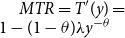 $MTR = T'(y)= 1-(1-\theta ) \lambda y^{-\theta }$
, and
 $ATR = T(y)/y = 1-\lambda y^{-\theta }$
. Thus, tax is progressive when
 $(1-\theta )\lambda y^{-\theta }\lt \lambda y^{-\theta }$
, or
 $\theta \gt 0$
. There is a break-even income
 $y_{non}$
, below which people receive net transfer (
 $T(y)\lt 0$
), and above which people pay net tax (
 $T(y)\gt 0$
). At this break-even income, both the ATR and the net tax are zero (
 $T(y_{non})=0$
), and the MTR is
 $\theta$
. This gives the break-even income
 $y_{non}=\lambda ^{1/\theta }$
, government tax revenue
 $\int _{y_{non}}^{\infty } (y-\lambda y^{1-\theta })d\Phi (a,x)$
, and transfer expenditure
 $\int _{0}^{y_{non}}(\lambda y^{1-\theta } -y)d\Phi (a,x)$
. Hereafter, we refer to this policy as the “nonlinear program.”
Negative income tax.
Under NIT, households with earned income higher than the threshold income
 ${\, \hat{\kern-1pt y}}$
pay tax for their excessive income
 $y-{\, \hat{\kern-1pt y}}$
with tax rate
 $\hat {\tau }$
. The disposable income of a household earning more than the threshold income is thus
 $y-\hat {\tau }(y-{\, \hat{\kern-1pt y}})$
. The collected taxes transfer to the households with income below the threshold income. Zero income households receive
 $T_{0}$
, and this transfer phases out with rate
 $\phi$
, which makes the disposable income
 $y+T_{0}-\phi y$
for incomes below the threshold. This makes the government’s total tax revenue
 $\int _{{\, \hat{\kern-1pt y}}}^{\infty } \hat {\tau }(y-{\, \hat{\kern-1pt y}}) d\Phi (a,x)$
, and the total transfer expenditure
 $\int _{0}^{{\, \hat{\kern-1pt y}}} (T_{0}-\phi y) d\Phi (a,x)$
. Moreover, the threshold income
 ${\, \hat{\kern-1pt y}}$
is smaller than that from the nonlinear program (
 $y_{non} \geq {\, \hat{\kern-1pt y}}$
), because the progressivity under the nonlinear program collects more tax from the high incomes than the linear tax
 $\hat {\tau }$
does under NIT. This indicates that more people receive net transfers from the nonlinear program, compared to NIT. We analytically show this in Proposition1 (see Section 2.2), then quantitatively show that the progressivity is higher than the linear tax rate for excessive incomes (
 $\theta \gt \hat {\tau }$
) in Table 3.
Universal basic income.
Under UBI, everyone faces the same tax rate
 $\tau$
for their income
 $y$
and receives a lump-sum cash transfer
 ${\, \bar{\kern-1pt T}}$
, which makes the disposable income of a household
 $y-\tau y+{\, \bar{\kern-1pt T}}$
. This gives the total tax revenue
 $\int _{0}^{\infty } \tau y d\Phi (a,x)$
, and the total transfer expenditure
 $\int _{0}^{\infty } {\, \bar{\kern-1pt T}} d\Phi (a,x)$
.
2.1.4 Equilibrium
A stationary competitive equilibrium is a set of prices and allocations consisting of value and policy functions
 $V(a,x)$
,
 $c(a,x)$
,
 $a'(a,x)$
, and
 $h(a,x)$
, factor prices
 $(w,r)$
, aggregate quantities
 $(K,L)$
, and the invariant distribution
 $\Phi (a,x)$
.
Households.
Given prices
 $(w,r)$
, the value function
 $V(a,x)$
and policy functions
 $c(a,x)$
,
 $a'(a,x)$
, and
 $h(a,x)$
solve the household’s dynamic optimization problem described in Section 2.1.1.
Firms.
Factor prices
 $(w,r)$
satisfy the firm’s profit maximization:
 \begin{align*} w &= \alpha (K/L)^{1-\alpha }, \\ r &= (1-\alpha )(K/L)^{-\alpha } - \delta . \end{align*}
Market clearing conditions. Factor markets and goods market clear as:
 \begin{align*} L &= \int x h(a,x) d\Phi (a,x), \\ K &= \int a d\Phi (a,x), \\ \int (c(a,x) + a'(a,x)) d\Phi (a,x) &= F(K,L) + (1-\delta )K. \end{align*}
Government. The government balances the budget in each policy, as described in Section 2.1.3.
Distribution.
The stationary distribution
 $\Phi (a,x)$
is consistent with individual behavior, in the sense that it is invariant under the policy function
 $a'(a,x)$
and the transition probability
 $\pi (x'|x)$
.
2.2 Theoretical analysis of the government budget
Building on the framework of Chang et al. (Reference Chang, Han and Kim2024), which formalizes and generalizes Mankiw (Reference Mankiw2021), we impose initially identical government budgets across policies, employing nonlinearity in addition. With endogenous transfer, the following holds for
 $t=0$
:
 \begin{align} &\underbrace {\int _{y_{non,t}}^{\infty } \big(y_{t}-\lambda _{t} y_{t}^{1-\theta }\big) d\Phi (a_{t},x_{t})=\int _{0}^{y_{non,t}} \big(\lambda _{t} y_{t}^{1-\theta } -y_{t} \big) d\Phi (a_{t},x_{t})}_{\text{nonlinear program}} \nonumber\\ &\quad = \underbrace {\hat {\tau }\int _{{\, \hat{\kern-1pt y}}}^{\infty }(y_{t}-{\, \hat{\kern-1pt y}}) d\Phi (a_{t},x_{t})=\int _{0}^{{\, \hat{\kern-1pt y}}}(T_{0,t}-\phi y_{t}) d\Phi (a_{t},x_{t})}_{\text{NIT}} \nonumber\\ &\quad = \underbrace {\tau \int _{0}^{\infty }y_{t}d\Phi (a_{t},x_{t})= \int _{0}^{\infty } \bar {T_{t}} d\Phi (a_{t},x_{t})}_{\text{UBI}}, \end{align}
and this holds only within the policy after the initial period.
Now we analytically show that the nonlinear program has higher threshold income than that of NIT at the initial period. That is, the upward political pressure of the threshold income under NIT can be relieved to some extent under the nonlinear program, and more households can benefit from the nonlinear program than from NIT. This is because the high-income households pay more tax under the nonlinear program than under NIT, which moves the threshold income upward so that the tax revenues and transfer amounts are equal.
Proposition 1.
The nonlinear tax-and-transfer program has higher break-even income than that from negative income tax:
 $y_{non} \geq {\, \hat{\kern-1pt y}}$
.
Proof.
Apply Jensen’s inequality and concavity. Suppose the NIT break-even income is the same as the average income (
 ${\, \hat{\kern-1pt y}}={\, \bar{\kern-1pt y}}$
). Let
 $g(y) \equiv y^{1-\theta }$
and
 $z \equiv \int yd\Phi (a,x)={\, \bar{\kern-1pt y}}$
. Since
 $0\lt \theta \lt 1$
and
 $g''(y)\lt 0, g$
is concave. Thus,
 $g(y) \leq g(z)+g'(z)(y-z)$
for all
 $y$
. Integrating both sides gives:
 $\int g(y)d\Phi (a,x) \leq \int g(z)d\Phi (a,x)=g(z)=z^{1-\theta }$
because
 $\int (y-z)d\Phi (a,x)=0$
. Now we have:
 $\int y^{1-\theta }d\Phi (a,x) \leq (\! \int yd\Phi (a,x))^{1-\theta }$
. Multiply both sides by
 $\lambda$
:
 $\int \lambda y^{1-\theta }d\Phi (a,x) \leq \lambda (\! \int yd\Phi (a,x))^{1-\theta }=\lambda {\, \bar{\kern-1pt y}}^{1-\theta }$
. Note that the integral of the net tax function is zero
 $0 = \int T(y)d\Phi (a,x)$
. Hence,
 ${\, \bar{\kern-1pt y}}-\int \lambda y^{1-\theta }d\Phi (a,x)=0$
, which is greater than or equal to
 ${\, \bar{\kern-1pt y}}-\lambda {\, \bar{\kern-1pt y}}^{1-\theta }$
as above. This gives
 ${\, \bar{\kern-1pt y}} \leq \lambda {\, \bar{\kern-1pt y}}^{1-\theta }$
, now divide both sides by
 ${\, \bar{\kern-1pt y}}^{1-\theta }$
and get:
 ${\, \bar{\kern-1pt y}}^{\theta } \leq \lambda$
. Since
 $\theta \gt 0$
,
 ${\, \bar{\kern-1pt y}} \leq \lambda ^{1/\theta }$
, where
 $\lambda ^{1/\theta }=y_{non}$
from the net tax function
 $T(y).$
Therefore,
 ${\, \bar{\kern-1pt y}}={\, \hat{\kern-1pt y}} \leq y_{non}$
.
Proposition1 holds as long as the NIT break-even income equals the average income (
 ${\, \hat{\kern-1pt y}}={\, \bar{\kern-1pt y}}$
). This setting balances the NIT government budget, and we show below that it also suffices to equalize government budgets across policies.
Before proceeding to the explicit analysis, we make two assumptions that equalize the initial level of total tax revenues and the total transfer expenditures across policies. The first assumption we make for the identical amount of tax revenues is that the tax rate under NIT and the phase-out rate are identical:
 $\hat {\tau }=\phi$
. This assumption differs from that of Chang et al. (Reference Chang, Han and Kim2024), where it assumes the same tax rates across UBI, NIT, and NIT’s phase-out rate (
 $\tau =\hat {\tau }=\phi$
). We take the
 $\hat {\tau }=\phi$
assumption, but we show that
 $\tau \neq \hat {\tau }$
, if we are to equal the tax revenues across NIT and UBI. For NIT tax revenue to match the UBI tax revenue in our framework, the NIT tax rate
 $\hat {\tau }$
must be higher than the UBI tax rate
 $\tau$
, because NIT collects tax only from the excessive incomes above the threshold income
 ${\, \hat{\kern-1pt y}}$
, whereas UBI collects tax from everyone. Formally, the NIT tax rate
 $\hat {\tau }$
that equalizes tax revenues across NIT and UBI is
 $\hat {\tau }=\tau {\, \bar{\kern-1pt y}}/\int _{{\, \hat{\kern-1pt y}}}^{\infty }(y-{\, \hat{\kern-1pt y}})d\Phi (a,x)$
. A simple manipulation leads to
 ${\tau }/{\hat {\tau }}=\int _{{\, \hat{\kern-1pt y}}}^{\infty }(y-{\, \hat{\kern-1pt y}})d\Phi (a,x)/{\int _{0}^{\infty }y d\Phi (a,x)}$
, where the RHS is smaller than 1. Therefore,
 $\tau \lt \hat {\tau }$
. This shows that the high-income households pay larger tax under NIT than under UBI, which could potentially lead to a larger reduction of labor supply and savings from high-income households.
The second assumption we make for the identical initial amount of transfer expenditures is that the NIT transfer for zero incomes is the same as the NIT tax rate on the average income:
 $T_{0}=\hat {\tau }{\, \bar{\kern-1pt y}}$
. As well as the tax rate case, this assumption differs from that of Chang et al. (Reference Chang, Han and Kim2024), where it assumes that the guaranteed minimum income under NIT equals the lump-sum transfer under UBI (
 $T_{0}={\, \bar{\kern-1pt T}}$
), where
 ${\, \bar{\kern-1pt T}}=\tau {\, \bar{\kern-1pt y}}$
from UBI government budget. We show that
 $T_{0} \neq {\, \bar{\kern-1pt T}}$
, if we are to equal the initial transfer amounts across NIT and UBI. Suppose the transfer expenditures equal across NIT and UBI as:
 ${\, \bar{\kern-1pt T}}=\int _{0}^{{\, \hat{\kern-1pt y}}}(T_{0}-\phi y)d\Phi (a,x)$
. If
 $T_{0}={\, \bar{\kern-1pt T}}$
, the RHS becomes
 $\tau {\, \bar{\kern-1pt y}} \psi - \int _{0}^{{\, \hat{\kern-1pt y}}} \hat {\tau }y d\Phi (a,x)$
because
 ${\, \bar{\kern-1pt T}}=\tau {\, \bar{\kern-1pt y}}$
from the balanced budget within UBI, and
 $\phi =\hat {\tau }$
from the first assumption, while
 $\psi \in [0,1]$
denoting the proportion of households under the threshold income. The equation becomes
 $\int _{0}^{{\, \hat{\kern-1pt y}}} \hat {\tau }y d\Phi (a,x)=\tau {\, \bar{\kern-1pt y}}(\psi -1)$
, which is a contradiction because the LHS here is positive and the RHS is negative. Therefore,
 $T_{0} \neq {\, \bar{\kern-1pt T}}$
. Moreover, using
 $\tau \lt \hat {\tau }$
from above and the second assumption, we know that
 $\hat {\tau }{\, \bar{\kern-1pt y}}=T_{0}\gt {\, \bar{\kern-1pt T}}=\tau {\, \bar{\kern-1pt y}}$
. This shows that the guaranteed minimum income is larger under NIT than under UBI in our framework, benefitting the low-income households more, which could potentially lead to a larger reduction of labor supply and savings from low-income households as they can insure their future income shocks better under NIT, which disincentivizes precautionary saving.
Using these two assumptions from above (
 $\hat {\tau }=\phi$
and
 $T_{0}=\hat {\tau }{\, \bar{\kern-1pt y}}$
), we now explicitly show that the setting used to close the NIT budget (
 ${\, \hat{\kern-1pt y}}={\, \bar{\kern-1pt y}}$
) in Proposition1 balances the government budgets across NIT and UBI as well. First, suppose the identical transfer expenditures:
 $\tau {\, \bar{\kern-1pt y}}=\hat {\tau } (\psi {\, \bar{\kern-1pt y}} - \int _{0}^{{\, \hat{\kern-1pt y}}}yd\Phi (a,x))$
. Divide both sides by
 $\hat {\tau }$
then rewrite as:
 $\int _{0}^{{\, \hat{\kern-1pt y}}}yd\Phi (a,x)={\, \bar{\kern-1pt y}}(\psi -(\tau /\hat {\tau }))$
. The identical tax revenues across NIT and UBI makes the RHS
 ${\, \bar{\kern-1pt y}}\psi -\int _{{\, \hat{\kern-1pt y}}}^{\infty }(y-{\, \hat{\kern-1pt y}})d\Phi (a,x)$
, using
 $\tau /\hat {\tau }$
. Rewrite this as:
 ${\, \bar{\kern-1pt y}}\psi -\int _{{\, \hat{\kern-1pt y}}}^{\infty }yd\Phi (a,x)+\int _{{\, \hat{\kern-1pt y}}}^{\infty } {\, \hat{\kern-1pt y}}d\Phi (a,x)$
. With the LHS
 $\int _{0}^{{\, \hat{\kern-1pt y}}}yd\Phi (a,x)$
, we have
 ${\, \bar{\kern-1pt y}}\psi =\int _{0}^{\infty }yd\Phi (a,x)-\int _{{\, \hat{\kern-1pt y}}}^{\infty }{\, \hat{\kern-1pt y}} d\Phi (a,x)={\, \bar{\kern-1pt y}}-\int _{{\, \hat{\kern-1pt y}}}^{\infty }{\, \hat{\kern-1pt y}} d\Phi (a,x)$
. This leads to:
 $\int _{{\, \hat{\kern-1pt y}}}^{\infty } {\, \hat{\kern-1pt y}} d\Phi (a,x)={\, \bar{\kern-1pt y}}(1-\psi )$
, where the LHS is
 ${\, \hat{\kern-1pt y}}(1-\psi )$
. Therefore,
 ${\, \hat{\kern-1pt y}}={\, \bar{\kern-1pt y}}$
.
The government that runs a balanced budget in each period has the following budget constraint. For all time
 $t$
, the nonlinear program has
 $\int _{y_{non,t}}^{\infty }(y_{t}-\lambda _{t} y_{t}^{1-\theta }) d\Phi (a_{t},x_{t})=\int _{0}^{y_{non,t}} (\lambda _{t} y_{t}^{1-\theta } -y_{t}) d\Phi (a_{t},x_{t})$
, NIT has
 $\hat {\tau }\int _{{\, \hat{\kern-1pt y}}}^{\infty }(y_{t}-{\, \hat{\kern-1pt y}}) d\Phi (a_{t},x_{t})=\int _{0}^{{\, \hat{\kern-1pt y}}}(T_{0,t}-\phi y_{t}) d\Phi (a_{t},x_{t})$
, and UBI has
 $\tau \int _{0}^{\infty }y_{t}d\Phi (a_{t},x_{t})= \int _{0}^{\infty } \bar {T_{t}} d\Phi (a_{t},x_{t})$
. That is, the tax parameters in each policy
 $\tau$
,
 $\hat {\tau }$
, and
 $\theta$
are set initially and held fixed across periods, whereas the transfer parameters are time-varying. Under each policy, the government adjusts transfer level
 $\lambda _{t}$
,
 $T_{0,t}$
, and
 ${\, \bar{\kern-1pt T}}_{t}$
, to satisfy the period-by-period budget balance. In particular, changes in
 $\lambda _{t}$
and
 ${\, \bar{\kern-1pt T}}_{t}$
imply changes in
 $y_{non,t}$
and
 $y_{t}$
, whereas the NIT threshold income
 ${\, \hat{\kern-1pt y}}$
, initially set equal to the baseline average income, is held fixed because of the political resistance to changing the threshold (see Friedman (Reference Friedman1968)). At the initial period, the calibration
 $T_{0}=\hat {\tau } {\, \bar{\kern-1pt y}}$
implies that
 ${\, \hat{\kern-1pt y}}$
coincides with the break-even income. In subsequent periods, the government adjusts
 $T_{0,t}$
such that the budget balances as tax base shrinks. Consequently, the break-even income need not coincide with the fixed threshold
 ${\, \hat{\kern-1pt y}}$
. After equalizing the government budgets across policies at the first period, each policy brings different levels of distortions in factor inputs and thus aggregate output (see Section 3). Accordingly, the size of the tax base declines, shrinking the size of total transfer for balanced budget, which converges as the economy reaches the steady state. In Section 5, we additionally study the case where the transfer rules (
 $\lambda$
,
 $T_{0}$
, and
 ${\, \bar{\kern-1pt T}}$
) are fixed. In that case, the fiscal parameters are not endogenously changing over time, which enables us to capture the tax deficit as the redistributive policies shrink the tax base.
2.3 Calibration
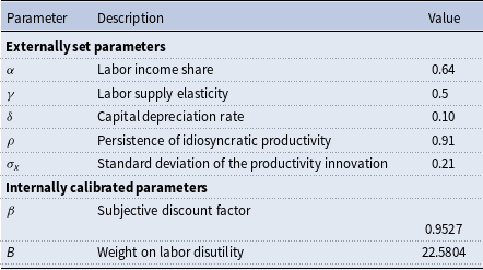
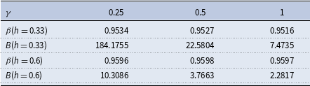
This subsection proceeds in four steps. First, Table 1 summarizes the externally set and internally calibrated parameters of the benchmark economy. Second, Table 2 examines how the internally calibrated values of
 $\beta$
and
 $B$
vary under alternative values of labor supply elasticity and average working hours. Third, Table 3 presents the fiscal parameters. Finally, we show the model’s distributional fit to the data in Table 4 and Figure 1.
Parameters of the benchmark economy

Table 1. Long description
A table comparing parameters of a benchmark economy. The table has 4 rows and 3 columns. Column headers are gamma, beta(h = 0.33), B(h = 0.33), beta(h = 0.6), and B(h = 0.6). Row labels are 0.25, 0.5, and 1. Row 1: gamma, 0.25; beta(h = 0.33), 0.9534; B(h = 0.33), 184.1755; beta(h = 0.6), 0.9596; B(h = 0.6), 10.3086. Row 2: gamma, 0.5; beta(h = 0.33), 0.9527; B(h = 0.33), 22.5804; beta(h = 0.6), 0.9598; B(h = 0.6), 3.7663. Row 3: gamma, 1; beta(h = 0.33), 0.9516; B(h = 0.33), 7.4735; beta(h = 0.6), 0.9597; B(h = 0.6), 2.2817.
In Table 1, the upper panel reports the externally set parameters, whose values are standard in the literature and taken from Chang et al. (Reference Chang, Han and Kim2024). The lower panel reports the parameters calibrated internally in our model to match the corresponding targets discussed throughout the paper.
The externally set parameters in Table 1 take the standard values in the literature. In the first-order Markov process for idiosyncratic income shock, we use the persistence
 $\rho =0.91$
and the standard deviation
 $\sigma _x=0.21$
as Chang et al. (Reference Chang, Han and Kim2024). We use the moderate labor supply elasticity as the baseline (
 $\gamma =0.5$
) and conduct the sensitivity analysis where labor is either inelastic (
 $\gamma =0.25$
) or elastic (
 $\gamma =1$
) in Section 4. The corresponding changes in internally calibrated parameters are reported in Table 2.
We internally calibrate the two parameters,
 $\beta$
and
 $B$
, to match the average real rate of return to capital of 4% and average working hours of 0.33, following Chang et al. (Reference Chang, Han and Kim2024). The former corresponds to the average real return to capital in the United States after the World War II. The latter corresponds to the fact that individuals spend, on average, about one third of their time endowment on work. Table 2 reports the calibrated values of
 $\beta$
and
 $B$
under alternative labor supply elasticities, for targeted average working hours of
 $h=0.33$
and
 $h=0.6$
. Targeting
 $h=0.6$
serves as a robustness check, since alternative definitions of time endowment can imply higher
 $h$
than the standard value
 $h=0.33$
. Under both targets (
 $h=0.33$
and
 $h=0.6$
), a larger
 $\gamma$
requires a smaller
 $B$
, indicating that their qualitative relationship is robust to the choice of the hours target.
 $\beta$
and
 $B$
for each labor elasticity and average working hours

Table 2. Long description
A table with four columns and six rows, detailing parameters of a benchmark economy. The columns are labeled Parameter, Description, Value, and Notes. The table is divided into two sections: Externally set parameters and Internally calibrated parameters. Row 1: Parameter, Labor income share; Description, empty; Value, 0.64; Notes, empty. Row 2: Parameter, Labor supply elasticity; Description, empty; Value, 0.5; Notes, empty. Row 3: Parameter, Capital depreciation rate; Description, empty; Value, 0.10; Notes, empty. Row 4: Parameter, Persistence of idiosyncratic productivity; Description, empty; Value, 0.91; Notes, empty. Row 5: Parameter, Standard deviation of the productivity innovation; Description, empty; Value, 0.21; Notes, empty. Row 6: Parameter, Subjective discount factor; Description, empty; Value, 0.9527; Notes, empty. Row 7: Parameter, Weight on labor disutility; Description, empty; Value, 22.5804; Notes, empty.
Notes: The labor supply elasticity
 $\gamma$
is set to 0.5 in the baseline calibration and varied to 0.25 and 1 for the sensitivity analysis.
Fiscal parameters.
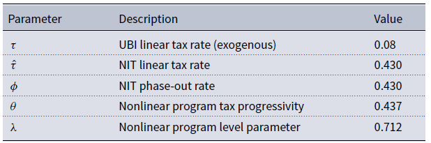
In Table 3, we exogenously set the UBI tax rate
 $\tau = 0.08$
, which is the welfare-maximizing rate in Chang et al. (Reference Chang, Han and Kim2024), then we compute the remaining fiscal parameters (
 $\hat {\tau },\phi ,\theta ,\lambda$
) so as to equalize the government budgets initially across policies (see Equation (2)). From the baseline economy, we get the average income
 ${\, \bar{\kern-1pt y}}$
. Setting UBI tax rate
 $\tau =0.08$
gives the lump-sum transfer
 ${\, \bar{\kern-1pt T}}=\tau {\, \bar{\kern-1pt y}}$
from the balanced government budget of UBI. As we have explained earlier in subsection 2.2, we balance the NIT government budget by setting the NIT threshold income equal to the baseline average income (
 ${\, \hat{\kern-1pt y}}={\, \bar{\kern-1pt y}}$
), under the assumptions that the NIT tax rate equals the transfer phase-out rate (
 $\hat {\tau }=\phi$
), and zero income households receive some proportion of the average income (
 $T_{0}=\hat {\tau }{\, \bar{\kern-1pt y}}$
). Then, we compute the tax rate
 $\hat {\tau }$
that equalizes the tax revenues across NIT and UBI:
 $\hat {\tau }=\tau {\, \bar{\kern-1pt y}}/\int _{{\, \hat{\kern-1pt y}}}^{\infty }(y-{\, \hat{\kern-1pt y}})d\Phi (a,x)$
. For the nonlinear program, the net tax function is
 $y-\lambda y^{1-\theta }$
. For any given
 $\theta$
, we compute
 $\lambda =E[y]/E[y^{1-\theta }]$
, where
 $E[y]={\, \bar{\kern-1pt y}}$
. With
 ${\, \bar{\kern-1pt y}}$
given from the baseline economy, this
 $\lambda$
ensures that the government budget is balanced under the nonlinear program (
 $E[y-\lambda y^{1-\theta }]=0$
). Given
 $\theta$
and the corresponding
 $\lambda$
, the break-even income at which the net tax is zero is
 $y_{non}=\lambda ^{1/\theta }$
. We then choose
 $\theta$
so that transfer expenditures equal across the nonlinear program and UBI:
 $\int _{0}^{\lambda ^{1/\theta }} \lambda y^{1-\theta }-y d\Phi (a,x)={\, \bar{\kern-1pt T}}=\tau {\, \bar{\kern-1pt y}}$
.
Fiscal parameters

Table 3. Long description
A table titled ‘Fiscal parameters’ with two main sections: Externally set parameters and Internally calibrated parameters. The table has three columns: Parameter, Description, and Value. Externally set parameters include Labor income share (alpha) with a value of 0.64, Labor supply elasticity (gamma) with a value of 0.5, Capital depreciation rate (delta) with a value of 0.10, Persistence of idiosyncratic productivity (rho) with a value of 0.91, and Standard deviation of the productivity innovation (sigma_x) with a value of 0.21. Internally calibrated parameters include Subjective discount factor (beta) with a value of 0.9527 and Weight on labor disutility (B) with a value of 22.5804.
Notes: The UBI tax rate
 $\tau$
is set exogenously to 0.08, corresponding to the welfare-maximizing UBI in Chang et al. (Reference Chang, Han and Kim2024). The remaining fiscal parameters are determined so that each policy finances the same initial transfer expenditure as the UBI.
Exogenously setting the UBI tax rate
 $\tau =0.08$
differs from the baseline setting in Chang et al. (Reference Chang, Han and Kim2024), which sets
 $\tau = 0.2$
. Importantly, adopting
 $\tau = 0.2$
in our framework numerically implies an unrealistically high NIT tax rate (
 $\hat {\tau }\gt 1$
), because NIT collects tax only for the excessive incomes above the threshold income, whereas UBI collects tax from everyone.Footnote
3
To equalize government budgets across policies, NIT requires an unreasonable tax rate from the high-income households. Such tax rates are outside the economically meaningful range and violate the internal consistency of the tax-and-transfer system in our framework. We therefore restrict attention to the welfare-maximizing rate
 $\tau = 0.08$
. Although this specific rate is dependent on the model structure of Chang et al. (Reference Chang, Han and Kim2024), the corresponding NIT tax rate and the tax progressivity under the nonlinear program in our framework are in the economically reasonable range, allowing for a well-defined comparison of policy mechanisms.
A similar issue arises when the progressivity parameter
 $\theta$
is fixed exogenously. For example, imposing a data-based estimate of progressivity from Heathcote et al. (Reference Heathcote, Storesletten and Violante2017) does not generate the same initial transfer expenditure as the optimal UBI in our framework. Therefore, instead of setting the tax progressivity exogenously, we allow the progressivity under the nonlinear program to adjust, enabling us to infer the degree of progressivity required to finance the optimal UBI. The implied progressivity can then be compared to data-driven progressivity, providing a useful reference for assessing how the redistribution by linear policies relates to the progressivity observed in the data.
Table 3 shows that, to equalize the initial transfer amount, NIT requires a substantially higher tax rate than UBI: 43% of each additional unit of income above the threshold is taxed, and an additional unit of income below the threshold reduces transfers by 43%. While Chang et al. (Reference Chang, Han and Kim2024) show that NIT can replicate the ex post distribution of UBI with the same tax rates (
 $\tau =\hat {\tau }=\phi$
), our calibration shows that NIT replicating the transfer expenditure of UBI requires a much higher tax rate. This brings larger distortions to factor inputs and thus aggregate output under NIT by discouraging labor supply, and disincentivizing the precautionary saving motives. The quantitative results are presented in Section 3, where we show the larger reduction of factor inputs and aggregate output under NIT and under the nonlinear program, compared to UBI.
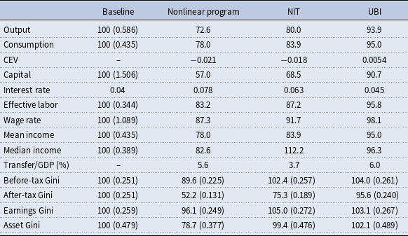
Under the nonlinear program, the implied degree of tax progressivity is substantially higher than in Heathcote et al. (Reference Heathcote, Storesletten and Violante2017), which estimates a U.S. tax progressivity parameter of 0.181 using PSID and TAXSIM data. This reflects the fact that, to finance the optimal UBI with a progressive taxation, the government must rely on much stronger tax progressivity to raise sufficient revenue. Similarly to NIT, this high progressivity brings a larger reduction in factor inputs and thus aggregate output. This is consistent with the existing argument that UBI is “costly” to implement. Quantitatively, Figure 2 and Table 5 in subsection 3.1 show that UBI requires the largest transfer share of GDP. However, we do not interpret this directly as more expensive, because distributions differ across policies after the policy implementation. Instead, we focus on the tax deficit in Section 5.
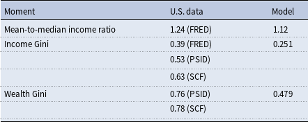
Distributional fit. Table 4 summarizes the distributional moments in the model and the U.S. data. Obtaining the data from the FRED, Figure 1 reports real mean and median household income over the period 1953–2024 (U.S. Census Bureau, 2025a, 2025b), and the income Gini index over the period 1963–2024 (U.S. Census Bureau, 2026). On average, real mean income is $92,085, while the real median income is $74,443, implying a mean-median income ratio of 1.24. In our model, mean income is 0.435 and median income is 0.389 (see Table 5), yielding a mean-median ratio of 1.12. The smaller mean-median ratio in our model indicates a less right-skewed income distribution and a thinner upper tail than observed in the data.
Distributional moments in the U.S. data and model

Table 4. Long description
A table comparing distributional moments in the U.S. data and model. The table has four rows and three columns. The columns are labeled ‘Moment’, ‘U.S. data’, and ‘Model’. The rows are labeled with different moments: Mean-to-median income ratio, Income Gini, and Wealth Gini. Each row provides values for the U.S. data and the model. For the Mean-to-median income ratio, the U.S. data shows 1.24 (FRED) and the model shows 1.12. For the Income Gini, the U.S. data shows 0.39 (FRED), 0.53 (PSID), and 0.63 (SCF), while the model shows 0.251. For the Wealth Gini, the U.S. data shows 0.76 (PSID) and 0.78 (SCF), and the model shows 0.479.
Notes: FRED denotes the Federal Reserve Economic Data database, PSID denotes the Panel Study of Income Dynamics, and SCF denotes the Survey of Consumer Finances.
U.S. mean income, median income, and income Gini index.
Notes: Data obtained from FRED. Real mean family income and real median family income data cover from 1953 to 2024, and income Gini index data covers from 1963 to 2024. See references for the link to the source.

The model generates relatively low income and asset Gini index values. This is a common limitation of models in which income heterogeneity is driven by a single source of idiosyncratic risk, because it restricts the amount of dispersion that can be generated at the upper end of the distribution (Benhabib et al. Reference Benhabib, Bisin and Zhu2011). This is also emphasized by Chang et al. (Reference Chang, Han and Kim2024), whose income and asset Gini values are 0.33 and 0.64, respectively. They also mention that their Gini index values are lower than the ones observed in the data. They report the U.S. Gini index values of 0.53 and 0.76 in the PSID, and 0.63 and 0.78 in the Survey of Consumer Finances, which we summarize in Table 4. Although the model underestimates inequality in levels, its main purpose is to compare the macroeconomic effects of redistributive policies, rather than to compare wealth concentration among the superrich. Therefore, we focus on how inequality measures respond to redistribution rather than on exactly matching their levels. Nevertheless, the model performs well in aggregate. The baseline economy generates a capital-output ratio of 2.57 (see Table 5), which is close to the values of 2.5 and 2.598 from Aiyagari and McGrattan (Reference Aiyagari and McGrattan1998) and Chang et al. (Reference Chang, Han and Kim2024), respectively.
Consistent with Chang et al. (Reference Chang, Han and Kim2024), redistribution in the model reduces income inequality while increasing asset inequality under UBI: the income Gini declines after redistribution, whereas the asset Gini rises due to changes in saving incentives (see Table 5). UBI shifts resources with relatively uniform marginal incentives, so its main effect is to provide insurance that weakens precautionary saving, which can tilt the wealth distribution toward greater concentration. However, asset inequality declines under the NIT and nonlinear programs. Under the NIT, transfers are targeted toward households with low current income and are financed by taxes on households above the income threshold. This compresses after-tax income and reduces the saving capacity of high-income, high-asset households, thereby limiting wealth accumulation at the top of the asset distribution. Although the income guarantee also weakens the precautionary saving motive of low-income households, the reduction in upper-tail asset accumulation dominates in the stationary distribution. In contrast, the HSV-style nonlinear tax schedule compresses disposable income through a net tax function, but it does not provide a strictly positive income floor for households with zero income. Thus, its insurance effect at the bottom is weaker than that of the NIT, even though it can still reduce asset inequality by lowering the dispersion of after-tax income and limiting asset accumulation among high-income households.
3. Results
In this Section, we first show the transition dynamics of the economy for 40 periods and provide a table for the new steady state values in subsection 3.1. Then we explain who benefits where and how in subsection 3.2, by comparing the households’ value gain after the redistribution relative to the baseline economy.
3.1 Transition dynamics and steady state outcomes
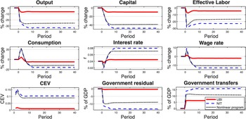
Assume the economy is in the steady state until the redistribution shock in period 1. At the initial period 0, the government plans a tax-and-transfer policy with the initial distribution in the old steady state. The transition paths of nonlinear program (black dotted line), NIT (blue dashed line), and UBI (red straight line) reach the new steady state, as presented in Figure 2.
Transition paths.
Notes: The red straight line corresponds to UBI, the blue dashed line to NIT, and the black dotted line to nonlinear program. We compute these transition paths by forward iteration. Given the factor prices
 $(w_{t-1},r_{t-1})$
, the cross-sectional distribution is updated using the Markov process and household policy rules obtained from value function iteration each period. Then, aggregate factor inputs
 $(K_t,L_t)$
are calculated, and prices are reset from the firm’s profit maximization problems.

While reaching the new steady state, aggregate effective labor plunges sharply then converges, whereas capital drifts down to the new steady state gradually. This occurs because the redistribution provides an insurance mechanism, reducing the work incentives and the precautionary saving motives of households.
Accordingly, the factor prices are either over- or undershooting as they depend on the ratio of labor and capital. In particular, interest rate increases if capital declines more than labor does. Here, interest rate first falls because a drop in labor depresses
 $L/K$
. Then, as labor recovers to some extent while capital continues its decline,
 $L/K$
rises and the interest rate rebounds above the pre-shock level. Conversely, the wage rate undershoots after a spike in
 $K/L$
pushing the wage rate up. It converges to the new steady state below the pre-shock level as the ratio
 $K/L$
starts decreasing.
Consumption jumps in the short-run because the lower interest rate makes current consumption relatively cheaper than future consumption. Since the economy’s long-run output is lower than the pre-shock level, expected future resources fall, so households cut back on spending and smooth consumption over time, pushing consumption below the pre-shock level.
Welfare outcomes are measured using consumption equivalent variation (CEV) in this balanced budget benchmark. CEV is defined as the percentage change in consumption that makes households indifferent between the policy economy and the laissez-faire baseline. CEV is computed from differences in value functions, weighted by the initial distribution. We report period-by-period CEVs, where these evaluations are intended to illustrate how short-run and long-run general equilibrium effects contribute to welfare differences. Early evaluations reflect short-run gains driven by consumption spikes, while evaluations based on later environments capture the long-run welfare loss. However under UBI, the welfare gains from redistribution dominate the associated welfare losses. Because the transfer is uniform and financed by a flat tax, the induced distortions to labor supply and savings are relatively mild, allowing long-run consumption to remain sufficiently high. As a result, the short-run welfare gains are not fully offset over time, leading to a positive CEV in the new steady state. In contrast, both the nonlinear program and NIT generate stronger distortions to labor and saving incentives. These distortions reduce aggregate factor inputs and depress long-run output and consumption more sharply. Although both policies gain welfare in the short run, the persistent decline in long-run consumption dominates, resulting in negative CEV.
Government transfers adjust endogenously over the transition as the government balances its budget every period. While the initial transfer amounts are matched across policies, subsequent movements in transfers are driven by changes in the tax base through endogenous responses of labor and capital, which emerges differences in transfer-to-GDP ratios as a consequence of general equilibrium effects. The transfer-to-GDP ratio remains lower under the nonlinear program and under NIT than under UBI, despite the fact that nonlinear program and NIT have larger reduction in aggregate output. This shows the stronger redistributive effects under the nonlinear program and under NIT, shrinking the tax base with higher tax rates.
Quantitatively in the long run, aggregate labor and capital decline by 16.8% and 43% under the nonlinear program, by 12.8% and 31.5% under NIT, and by 4.2% and 9.3% under UBI. Consistent with these factor responses, aggregate output falls by 27.4% under the nonlinear program, 20% under NIT, and 6.1% under UBI. Despite these larger output reductions, transfer expenditures amount to only 5.6% of GDP under the nonlinear program and 3.7% under NIT, compared with 6% under UBI, as reported in Table 5. These results indicate that differences in transfer burdens across policies are not mechanically driven by aggregate output losses, but instead reflect differences in the equilibrium scale of redistribution implied by each policy design.
Steady state outcomes (levels)

Table 5. Long description
A table comparing steady state outcomes across different economic programs. The table has 12 rows and 5 columns. Column headers are Baseline, Nonlinear program, NIT, and UBI. Row labels include Output, Consumption, CEV, Capital, Interest rate, Effective labor, Wage rate, Mean income, Median income, Transfer/GDP (percent), Before-tax Gini, After-tax Gini, Earnings Gini, and Asset Gini. Row 1: Output, 100 (0.586), 72.6, 80.0, 93.9. Row 2: Consumption, 100 (0.435), 78.0, 83.9, 95.0. Row 3: CEV, 0.021, 0.018, 0.0054. Row 4: Capital, 100 (1.506), 57.0, 68.5, 90.7. Row 5: Interest rate, 0.04, 0.078, 0.063, 0.045. Row 6: Effective labor, 100 (0.344), 83.2, 87.2, 95.8. Row 7: Wage rate, 100 (1.089), 87.3, 91.7, 98.1. Row 8: Mean income, 100 (0.435), 78.0, 83.9, 95.0. Row 9: Median income, 100 (0.389), 82.6, 112.2, 96.3. Row 10: Transfer/GDP (percent), 5.6, 3.7, 6.0. Row 11: Before-tax Gini, 100 (0.251), 89.6 (0.225), 102.4 (0.257), 104.0 (0.261). Row 12: After-tax Gini, 100 (0.251), 52.2 (0.131), 75.3 (0.189), 95.6 (0.240). Row 13: Earnings Gini, 100 (0.259), 96.1 (0.249), 105.0 (0.272), 103.1 (0.267). Row 14: Asset Gini, 100 (0.479), 78.7 (0.377), 99.4 (0.476), 102.1 (0.489).
Notes: The variables are normalized to 100 in the baseline, except for interest rate and CEV.
3.2 Household value gains
To complement the aggregate welfare analysis in the balanced budget benchmark, we examine how redistribution affects households across the state space. Figure 3 compares value functions relative to the baseline under each policy: the nonlinear program (top row), NIT (middle row), and UBI (bottom row), for inelastic, moderate, and elastic labor supply elasticities over the state space of asset holdings and productivity.
Household value gains.
Notes: Household value gains are measured as the difference in the value function, relative to the laissez-faire baseline for each policy (see Equation (1) for
 $V(a,x)$
). The x-axis indicates asset holdings
 $a$
, and the y-axis represents the productivity state
 $x$
. The black dashed line in each plot delineates the area of value loss. The first row corresponds to nonlinear program, the second row to NIT, and the third row to UBI. The first column presents results under inelastic labor, the second under moderate labor elasticity, and the third under elastic labor.

Compared to UBI on the bottom row, households with large asset holdings experience higher value gains under NIT and the nonlinear program, reflecting the larger increase in the equilibrium interest rate and the resulting rise in capital income. Since the return on capital scales with asset holdings, this channel favors high-asset households under NIT and nonlinear program. However, among these households, those with high productivity are worse off under NIT and the nonlinear program, as higher labor income is subject to higher taxation, whereas they benefit from UBI through relatively smaller tax and lump-sum transfers. For low-asset households, value gains from redistribution arise primarily among those with low productivity, for whom transfers dominate labor income distortions. When labor supply is elastic (
 $\gamma = 1$
), this pattern weakens: even low-asset, low-productivity households experience value losses under NIT and the nonlinear program.
Overall, Figure 3 indicates that UBI generates relatively broader value gains across the state space, with fewer households experiencing value losses. In contrast, NIT and the nonlinear program produce more heterogeneous outcomes. This contrast reflects the different nature of redistribution across policies. UBI provides uniform transfers that smooth value gains across households, whereas NIT and nonlinear redistribution concentrate gains and losses more sharply.
4. Sensitivity analysis
To this point, we have examined transition dynamics, the new steady state outcomes, and household value gains under each policy. In this Section, we now check the robustness of the results under changes in two parameters: labor supply elasticity
 $\gamma$
, and the targeted average working hours
 $h$
in the benchmark economy. We show that the macroeconomic results are affected by these parameters only quantitatively, not qualitatively.Footnote
4
First of all, we show the transition paths of the macroeconomic variables with inelastic and elastic labor supply elasticities (
 $\gamma \in \{0.25,1\}$
) in Figures A.1 and A.2. We then show value gains of households when the average working hours is targeted to be 0.6 in the benchmark economy in Figure A.5, for each labor supply elasticity. As we calibrate discount factor
 $\beta$
and labor disutility
 $B$
to match the target interest rate and average working hours, we repeat this calibration for each set of parameters in Table 2. In Figures A.1 and A.2, we plot the transition paths of the macroeconomic variables under two labor supply elasticities in which the top six panels apply inelastic labor and the bottom six panels elastic labor. Figures A.3 and A.4 repeat this exercise for a targeted average working hours of 0.6. Although a more elastic labor supply increases or decreases the size of the responses, the direction, shape, and relative ranking of each variable’s transition path remain unchanged. This indicates that our findings in Section 3 are robust to the choice of parameters, varying only in magnitude but not in form as well as the values in the new steady state in Table 5. Although the macroeconomic intuitions are not dependent on the labor supply elasticities, the household value gains in Figure A.5 are affected by the labor elasticities when the targeted average working hours is 0.6 in the benchmark economy.
When labor supply is inelastic or moderate (
 $\gamma =0.25$
or
 $\gamma =0.5$
), value gains under both the NIT and the nonlinear program are concentrated among households with low productivity. In these cases, redistribution primarily benefits households that receive substantial net transfers, while households with middle or high-productivity experience no gains regardless of their asset holdings. The phase-out structure implies that transfer incidence declines rapidly with productivity, and limited labor supply responses prevent middle-productivity households from offsetting this effect. In contrast, value gains extend beyond low-productivity households when labor supply is inelastic or moderate under UBI. In particular, households with middle-productivity experience positive value gains across a wide range of asset holdings. This reflects the uniform transfer structure of UBI, which provides insurance benefits that do not diminish with productivity and therefore benefit a broader segment of the productivity distribution.
When labor supply is elastic (
 $\gamma =1$
), the households’ welfare implications change substantially. Under both the NIT and the nonlinear program, households with low-asset holdings experience value losses even at low-productivity levels. Although these households can adjust labor supply in response to redistribution, their limited asset positions prevent them from benefiting from the higher return on capital, making capital income gains insufficient. Under UBI, low-asset households continue to experience value gains even when labor supply is elastic. However, for households with very high productivity, positive value gains arise if asset holdings are sufficiently large. In this case, asset income gains can outweigh labor income losses, whereas high-productivity households with limited assets remain worse off. These patterns indicate that, with elastic labor supply, asset holdings become a necessary condition for high-productivity households to benefit from redistribution under UBI, while low-asset households remain disadvantaged under the nonlinear program regardless of the productivity level.
As we equalize the initial amount of transfer expenditures across policies, the fiscal rebalancing itself is inherently policy-specific and may interact with redistribution in ways that are difficult to disentangle. To see the pure redistributive effects, Section 5 considers an alternative environment in which transfer rules are held fixed and government budgets are not endogenously changing.
5. Redistribution without fiscal rebalancing
Motivated by the Congressional Research Service report of Austin (Reference Austin2023) that shows federal deficit, we measure how much tax deficit each policy brings, by shutting down endogenous fiscal rebalancing. Redistribution reduces aggregate labor, capital accumulation, and output, shrinking the tax base, which eventually causes tax deficit when the transfer rules are held fixed. The resulting mismatch between tax revenues and transfer expenditures shows up as a government budget residual along the transition path in Figure A.6. This residual implies that the aggregate resource constraint does not hold exactly in the goods market, but household and firm decisions, prices, and the cross-sectional distribution remain internally consistent with the general equilibrium structure. This interpretation follows the spirit of disequilibrium analyses, which treat allocations under nonclearing constraints as informative objects (see Barro and Grossman (Reference Barro and Grossman1971); Mankiw (Reference Mankiw2006)).
By construction, budgets are balanced at
 $t=0$
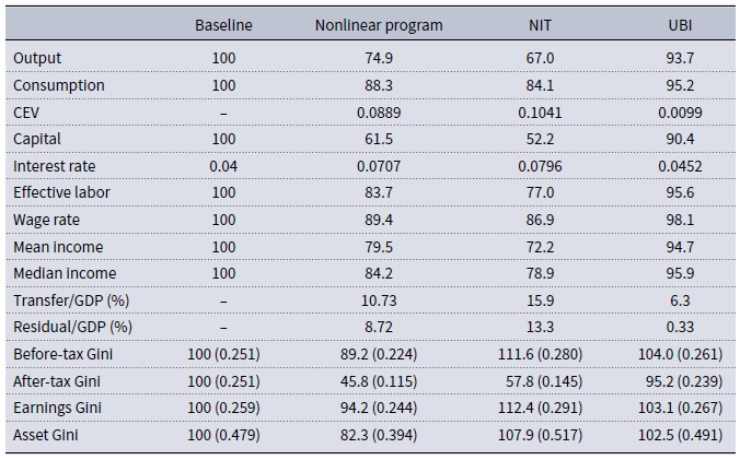
within and across policies because Equation (2) holds under the initial income distribution. After the redistribution shock, the tax base shrinks and deficits emerge because transfer rules are kept constant in this exercise. Quantitatively, aggregate labor and capital fall by 16.3% and 38.5% under the nonlinear program, 23.0% and 47.8% under NIT, and 4.4% and 9.6% under UBI. Aggregate output declines by 25.1% (nonlinear), 33.0% (NIT), and 6.3% (UBI). These output responses map into transfer-to-GDP ratios as: 10.73% under the nonlinear program, 15.9% under NIT, and 6.3% under UBI. The fiscal residuals also differ markedly. As a share of GDP, the residual is 8.72% under the nonlinear program, 13.3% under NIT, and 0.33% under UBI. These rankings mirror the size of the induced tax base shrinkage: UBI generates the smallest residual because it has the weakest impact on labor supply and capital accumulation, while NIT generates the largest residual because it produces the strongest distortion. The nonlinear program lies between the two.
Welfare measured by CEV is positive in all three policies. However, because the government runs a deficit by construction in this fixed transfer rule exercise, we do not interpret this CEV as a fully resource-feasible measure of aggregate welfare. We therefore focus on the cross-sectional pattern of household value gains. Figure A.7 shows that average household value gains are larger under the nonlinear program and NIT than under UBI. The nonlinear program delivers a conditional Pareto improvement: with moderate labor elasticity (
 $\gamma =0.5$
), a fiscal residual of 8.72% of GDP (see Table B.1) is associated with value gains for all households under the nonlinear program. While the gains for low-productivity households are smaller than under NIT, the qualitative pattern is similar on average across the labor elasticities.
The rise in interest rate is the most pronounced under NIT, generating larger capital income gains for asset-rich households. However, these households do not always gain more than low-asset households: when labor supply is not elastic (
 $\gamma \neq 1$
), low-asset, low-productivity households can experience larger gains because the marginal value of reduced taxes (or higher net transfers) is particularly high for them. Also, the reduction of labor supply is the most pronounced under NIT, which raises utility through lower disutility from work. This channel also explains why some low- to middle-asset households with middle- to high-productivity can lose under UBI but gain under NIT: they receive limited insurance from the uniform transfer while still paying relatively high taxes, whereas under NIT they benefit more from the transfer and from working less. In contrast, very low-asset households with very high productivity can remain worse off even under NIT unless labor supply is sufficiently elastic (
 $\gamma =1$
), in which case they can adjust hours more flexibly in response to the policy.
6. Conclusions
This paper compares nonlinear tax-and-transfer policy with the conventional linear policies (NIT and UBI) à la Aiyagari, and shows that the nonlinear policy distorts macroeconomy more than the linear policies do. Our comparison holds the initial transfer expenditures across policies fixed, motivated by the “autopilot” feature of the U.S. income-support programs. With the baseline economy calibrated to approximate the U.S. income distribution, we show that the tax progressivity needed to finance the optimal UBI more than doubles that from the data. Likewise, the NIT tax rate required to finance the optimal UBI is significantly high (43%). We summarize the quantitative findings below.
When initial transfer expenditures are equalized across policies, the nonlinear program requires a strong increase in progressivity (
 $\theta =0.437$
vs. 0.181 in Heathcote et al. (Reference Heathcote, Storesletten and Violante2017)) and generates larger distortions in the macroeconomy than the conventional linear policies (output declines by 27.4% under the nonlinear program, 20% under NIT, and 6.1% under UBI). Also, the transfer-to-GDP ratio adds up to 5.6% under the nonlinear program, which is more than under NIT (3.7%) but less than under UBI (6%). This shows that the conditionality shrinks the tax base relatively more than it reduces aggregate output, compared to the unconditional case. All three policies show short term welfare gain in aggregate, and the households with high-asset and low-productivity are better off after redistribution regardless of the policy.
With fixed transfer rules, redistributive distortions are most pronounced under NIT. The transfer-to-GDP ratio is 15.9%, higher than under the nonlinear program (10.73%) and under UBI (6.3%). Consistent with this, NIT implies a tax deficit of 13.3% of GDP, compared with 8.72% under the nonlinear program and 0.33% under UBI. These results suggest that, to keep costs contained, conditional programs must eventually be adjusted. For example, NIT can be feasible by lowering the threshold income (so that fewer households qualify) or by reducing the guaranteed minimum income. Lastly, the nonlinear program can deliver a conditional Pareto improvement, but only at the cost of an 8.72% tax deficit relative to GDP. Unless financed through other means, this conditional Pareto improvement is not resource-feasible and thus should not be interpreted as an implementable welfare improvement.
Future research could enrich the policy space by functionizing the fiscal parameters such as NIT’s phase-out rate or MTR, so that it can vary nonlinearly with income. This would compare conventional NIT with more flexible designs, and quantify how additional curvature in the policy affects the macroeconomy and welfare implications.
Competing interests
The author(s) declare none.
Use of AI
We used the generative AI ChatGPT-5.4 to improve language. After using this tool, we reviewed and edited the content as needed. We take full responsibility for this article.
Appendix A. Transition dynamics and value gains
Transition paths (target
 $h=0.33,\gamma =0.25$
).

Transition paths (target
 $h=0.33,\gamma =1$
).

Transition paths (target
 $h=0.6,\gamma =0.25$
).

Transition paths (target
 $h=0.6,\gamma =1$
).

Value gains for each labor elasticity (
 $h=0.6$
).

Transition paths without fiscal rebalancing.

Household value gains without fiscal rebalancing.

Appendix B. Tables of values in the new steady state
Steady state outcomes without fiscal rebalancing (levels)

Table B1. Long description
A table comparing economic outcomes under different policies. The table has 12 rows and 5 columns. The columns are labeled Baseline, Nonlinear program, NIT, and UBI. The rows are labeled Output, Consumption, CEV, Capital, Interest rate, Effective labor, Wage rate, Mean income, Median income, Transfer/GDP (percent), Residual/GDP (percent), Before-tax Gini, After-tax Gini, Earnings Gini, and Asset Gini. Each cell contains a numerical value representing the economic outcome under the respective policy. Notable trends include higher values under UBI for most metrics compared to other policies.
Notes: The variables are normalized to 100 in the baseline, except for interest rate and CEV.


 β
 B


 (wt−1,rt−1)
 (Kt,Lt)

 V(a,x)
 a
 x

 h=0.33,γ=0.25

 h=0.33,γ=1

 h=0.6,γ=0.25

 h=0.6,γ=1

 h=0.6


 Open access

