1. Introduction
International environmental problems featuring pollution spillovers such as climate change pose a special challenge since they have special features that distinguish them from national environmental problems. Electricity production provides a natural example of this sort of interaction: imports of electricity into developed countries like England and Germany can come from transitioning Eastern European countries such as Poland. Aside from the trans-boundary effects related to Polish carbon emissions, there are potentially very different perspectives on the significance of any future effects. These effects, together with the absence of an international agency with the authority to assess a carbon tax, combine to complicate the problem quite significantly. In particular, the importing (developed) country and the exporting (transitioning) country are likely to value the externality differently. In this context, feed-in tariffs or border tax adjustments can serve as a ‘second-best’ instrument to limit the transboundary pollution externality, playing a role for cross-border externalities that is somewhat similar to the role played by a Pigouvian tax.Footnote 1
A handful of authors have explored the potential use of trade instruments to control environmental externalities (Markusen, Reference Markusen1975a, Reference Markusen1975b; Baumol and Oates, Reference Baumol and Oates1988; Parry and Oates, Reference Parry and Oates2000); as a general rule, this extant literature has employed a static framework. But by its very nature the climate change problem is dynamic: environmental damages depend primarily on an accumulated stock, and they occur over a long time frame. There is also an existing literature that investigates the strategic incentives in transboundary pollution problems by using dynamic games. In these games, the players, usually the governments of countries, care about the stock of pollution, i.e., as pollution accumulates it affects the payoff to each country. Generally, the focus of these studies is a comparison between the cooperative scenario, which assumes a high degree of commitment to follow the agreed-upon pollution regulations, and the non-cooperative scenario, in which each country's environmental policy is selected to promote its own interest, given the other country's emission standards (Dockner and van Long, Reference Dockner and van Long1993; Mason, Reference Mason1997; Maler and de Zeeuw, Reference Maler and de Zeeuw1998; Dockner et al., Reference Dockner, Jorgensen, van Long and Sorger2000; List and Mason, Reference List and Mason2001; Bayramoglu, Reference Bayramoglu2006). This literature typically neglects the potential for a trade relationship among the countries involved in the transboundary pollution stock control.Footnote 2
Our goal in this paper is to analyze the interaction between a transitioning country that produces a carbon-intensive product and a developed country that consumes that product, paying particular attention to the role a feed-in tariff can play as a second-best instrument for controlling pollution stock externalities. The nature of the two economies has implications for their perspective on the future: the latent uncertainty within the transitioning economy arguably lowers the weight it places upon future effects; equivalently, one can think of this country as placing a smaller value on the future damages associated with climate change. As a stark limit to such a strategic environment, one might think of the exporting country as completely ignoring climate change effects. We derive the second-best optimal tariff-cum-border tax adjustment in this context, and show how it can be related to the current pollution stock. In this way, our results describe a methodology for crafting a carbon tax in terms of the atmospheric carbon stock.Footnote 3
We develop a dynamic model to investigate the role that border tax adjustments can play in the climate change problem. Two countries, U and D, are both producing the same single good and production in each country results in by-product emissions.Footnote 4 We assume a unidirectional flow of trade, with U exporting to D. Carbon emissions produced in both countries contribute to the common atmospheric stock. Because these damages become important over time, the relative weighting of future effects between the two countries is a potentially important concern, particularly when (as we envision) country U is in transition while country D is developed. This distinction manifests itself in terms of divergent evaluations of the future damages associated with climate change; we adopt the limiting view of this asymmetry wherein D cares about climate change but U does not.Footnote 5 In this framework, D applies a tariff-cum-border tax adjustment against imports as an indirect measure to control the carbon externality. We derive the second-best border tax, and show how it can be related to the carbon stock. We then extend the analysis to allow for potential short-run damages in U. Under some circumstances, this extension does not impact the sequence of tariffs charged by D, and hence U's resulting rate of production and the corresponding flow of carbon emissions. Under other circumstances, flow damages in U cause D to increase the border tax adjustment to a constant level where U's output equates marginal consumption benefits with the sum of marginal production costs and induced marginal damages. In such a scenario, both countries select a sequence of actions that are atemporal, and the resulting steady-state carbon stock is smaller than in the case without flow damages in U.
2. A dynamic model with border tax adjustments
Two countries, D and U, each produce a single consumption good, Q i (t), with a given fixed endowment of factors of production and a given technology, where i = d for country D and i = u for country U. Consumers are homogeneous within each country, but may be heterogeneous across countries. Production of the consumption good in each country results in a flow of carbon emissions that are linked to output. For simplicity we assume a fixed proportions relation, where each unit of output generates ϕ units of emissions for both D and U. The combined amount of carbon emissions contributes to the atmospheric carbon stock, Z. The evolution of the atmospheric carbon stock is described by the following equation of motion:
 $$\dot{Z} \lpar t\rpar = \phi Q\lpar t\rpar - kZ \lpar t\rpar \comma \;$$
where k represents the rate decay of the atmospheric stock and Q(t) = Q u (t) + Q d (t) is the combined output at time t. The initial level of the pollution stock is Z(0) = Z 0.
The stock of carbon generates damages associated with climate change, which we denote by the function Δ(Z); we assume Δ is increasing and strictly convex. Although both countries generate emissions, we assume that only D cares about damages from climate change. For now, we also assume that U does not suffer any damages from its emissions or the carbon stock; this assumption is relaxed in section 5. Without a supranational authority that can force U to change its emissions, D has no direct remedy to address the trans-boundary externality. It can, however, indirectly address the climate change externality by imposing a feed-in tariff or border tax, τ, on imports Y from U. The choice of the tariff affects the level of output in both countries: while it discourages production in U it creates an advantage for producers in D – thus increasing their output level. We assume the net effect of imposing a tariff-cum-border tax is to decrease the aggregate flow of carbon emissions. Following the standard assumption of the ‘second-best’ trade and environment literature, D is assumed to have sufficient market power to influence the terms of trade through its tariff. Because D suffers damages from the stock of the pollutant, some of which arises from production in D, it may also choose to levy an effluent tax, F d , upon domestic production.
The equilibrium price in D is determined by the combination of feed-in tariff and domestic tax in D, and so this price can be expressed as p(τ, F
d
). The effect of the tariff can be summarized as follows:
 ${\partial Q_d \over \partial \tau} \gt 0\comma \; {\partial Q_u \over \partial \tau} \lt 0\comma \; {\partial Y \over \partial \tau} \lt 0\comma \; {\partial p \over \partial \tau} \in \lpar 0\comma \; 1\rpar $
, i.e., a tariff lowers output in U and exports Y, raises output in D, and raises price by less than the amount of the tariff. The effects of the domestic carbon tax in D run mostly opposite to the feed-in tariff:
 ${\partial Q_d \over \partial F_d} \lt 0\comma \; {\partial Q_u \over \partial F_d} \gt 0\comma \; {\partial Y \over \partial F_{d}} \gt 0\comma \; {\partial p \over \partial F_d} \in \lpar 0\comma \; 1\rpar .$
Since an increase in the magnitude of either instrument causes an increase in price, combined output must fall – which then implies lower emissions. Note that, given our specification of p, we consider the impact of the tariff in lowering output in U to include any terms of trade effect.
Our measure of welfare for each country is its net surplusFootnote 6 ; for country U this is given by
 $$W_u \equiv \omega_u \lpar Q_u - Y\rpar - C_u \lpar Q_u\rpar + \lpar p - \tau\rpar Y\comma \;$$
where ω u represents gross consumer benefits (i.e., the area under the inverse demand curve) and C u is U's production cost function. Net benefits for D are given by the sum of its net surplus and the tariff revenue, less the damages from climate changeFootnote 7 :
 $$W_d \equiv \omega_d \lpar Q_d +Y\rpar - C_d \lpar Q_d\rpar - \lpar p - \tau\rpar Y - \Delta \lpar Z\rpar \comma \;$$
where ω d represents gross consumer benefits and C d represents production costs in D.
Given any value of the tariff and domestic tax in D, the market-clearing conditions for outputs are:
 $$\eqalign{\omega_{d}^{\prime} \lpar Q_{d} +Y\rpar &= p = C_{d}^{\prime} \lpar Q_d\rpar + F_d \semicolon \; \cr \omega_{u}^{\prime} \lpar Q_{u} -Y\rpar & = p - \tau = C_{u}^{\prime} \lpar Q_u\rpar .}$$
Because equilibrium outputs, exports and the post-tariff price are all functions of the feed-in tariff and domestic tax in D, net payoffs can be regarded as functions of τ and F d .
3. Optimal border taxes
In this section, we discuss three variants of the problem of determining the optimal time path of production and pollution. In the first, we investigate the cooperative solution. Then we investigate D's non-cooperative problem; there are two sub-cases here. In the first, we analyze the problem of setting optimal border taxes when domestic firms are assessed for a carbon tax. This can be thought of as the general problem confronting D; under some circumstances, it can be optimal to set the domestic tax equal to zero. In such an event, D's problem is somewhat simpler, in that it only chooses one instrument.
3.1. The socially optimal solution
We suppose there is a global social planner, whose goal is to choose time paths of outputs Q k for the two countries, along with a time path of trade, Y, so as to maximize the discounted flow of combined payoffs. These combined payoffs equal the sum of the two countries' utilities, less combined production costs and pollution damages. This solution requires setting outputs so as to satisfy the equi-marginal principle; this rule ensures that any aggregate output is produced at minimal cost. We can then construct the aggregate cost function C(Q) = C u (Q u ) + C d (Q d ), where Q = Q u + Q d and the equi-marginal principle, C u ′ (Q u ) = C d ′ (Q d ) = C′(Q), applies. Similarly, for any aggregated output, marginal utilities in the two countries must be equated, i.e., ω u ′ = ω d ′; this ensures that maximal gross benefits are obtained. Accordingly, we may define the aggregate benefit function
 $$u\lpar Q\rpar = \omega_u \lpar Q_u - Y\rpar + \omega_d \lpar Q_d + Y\rpar \comma \;$$
where Y is chosen so as to set ω
u
′(Q
u
− Y) = ω
d
′(Q
d
+ Y) = u′(Q). Armed with these constructs, one can re-interpret the cooperative problem as the choice of a time path of aggregate output that maximizes the discounted flow of aggregate benefits less aggregate costs and pollution damages. The current-value Hamiltonian for the cooperative problem is then
 ${\cal H}_{c} = u\lpar Q\rpar - C\lpar Q\rpar - \Delta\lpar Z\rpar + m \lpar \phi Q - kZ\rpar $
, where m is the (cooperative) shadow value of the pollution stock; as pollution is a bad, one presumes that m is negative. The corresponding optimality rule for the cooperative solution is
 $$u^{\prime}\lpar Q\rpar - C^{\prime}\lpar Q\rpar + \phi m = 0.$$
Interpreting marginal utility as price, equation (4) implies that rents (price less marginal cost) be equated to −ϕ m, the imputed marginal damage from a one-unit increase in the carbon stock. The solution also requires that the evolution of the shadow value satisfies
 $$\dot{m} = \lpar r + k\rpar m + \Delta^{\prime} \lpar Z\rpar \comma \;$$
where r is the (common) discount rate.Footnote 8
To determine the evolution of the socially optimal quantity we time-differentiate equation (4) and manipulate to obtain:
 $$\dot{Q} = {\lpar r + k\rpar \lpar u^{\prime} \lpar Q\rpar - C^{\prime}\lpar Q\rpar \rpar - \phi \Delta^{\prime}\lpar Z\rpar \over u^{\prime \prime}\lpar Q\rpar - C^{\prime \prime}\lpar Q\rpar }.$$
The steady state associated with this problem entails the combination (Q*, Z*) that solves
 $$u^{\prime}\lpar Q^{\ast}\rpar - C^{\prime} \lpar Q^{\ast}\rpar = {\phi \Delta^{\prime} \lpar Z^{\ast}\rpar \over r + k}\semicolon \;$$
 $$Q^{\ast} = {k \over \phi}Z^{\ast}.$$
In addition, we note that the long-run shadow value of the pollution stock for this problem is
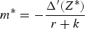 $m^{\ast} = -{\Delta^{\prime}\lpar Z^{\ast}\rpar \over r+k}$
. Interpreting −ϕ m* as the level of a pollution tax, the long-run equilibrium condition for the socially optimal level of production requires that marginal utility be set equal to the sum of marginal production cost plus this tax. As marginal utilities are equal in the two countries, as are marginal production costs, all producers – in both countries – pay the same tax (which corresponds to the capitalized value of long-run imputed pollution stock marginal damages).
The globally optimal path is comparable to those found in earlier papers on transboundary pollution problems. As in this subsection, these earlier studies generally assume the existence of an overarching regulatory authority that can control emissions (Dockner and van Long, Reference Dockner and van Long1993; Mason, Reference Mason1997; Maler and de Zeeuw, Reference Maler and de Zeeuw1998; Dockner et al., Reference Dockner, Jorgensen, van Long and Sorger2000). This central authority chooses the rate of emissions for both of the countries, with the goal of maximizing the joint welfare of the two regions. In our setting, one can think of the socially optimal time path of emissions as induced by levying a carbon tax on firms in both countries. To maintain the equality of marginal costs between the two countries, the same tax would need to be applied to all firms. This common tax can be inferred from the first-order condition, since the optimal static behavior for any firm is to set marginal cost equal to price less any tax; accordingly, the optimal tax corresponds to the wedge between price and marginal cost. Referring back to equation (4), this tax equals −ϕ m, the product of the magnitude of the shadow value of the pollution stock with the marginal impact of production upon the flow of emissions. Because the global planner's problem is equivalent to that of selecting outputs for the two countries, the marginal impact of D's production upon the combined payoffs must vanish.
3.2. D's non-cooperative problem
D's (non-cooperative) optimization problem entails choosing the time paths of the domestic carbon tax and the tariff-cum-border tax to maximize the discounted flow of its net benefit function over time. The current-value Hamiltonian for this optimization problem can be written as
 ${\cal H} = W_{d} \lpar \tau\comma \; F_d\rpar - \Delta\lpar Z\rpar + \theta \lsqb \phi Q \lpar \tau\comma \; F_d\rpar - kZ\rsqb $
, where θ is the shadow value of pollution. The necessary conditions for the maximum principle are
 $${\partial W_d \over \partial F_d} \le - \theta \phi {\partial Q \over \partial F_d}\semicolon \;$$
 $${\partial W_d \over \partial \tau} \le - \theta \phi {\partial Q \over \partial \tau}\semicolon \;$$
 $$\dot{\theta} = \lpar r + k\rpar \theta + \Delta^{\prime} \lpar Z\rpar \semicolon \;$$
as well as the transversality condition
 $\mathop{\lim}\limits_{t \rightarrow \infty} \theta \lpar t\rpar Z\lpar t\rpar e^{-rt} = 0$
. We assume that the local tax and border-tax must be non-negative. If F
d
is strictly positive, then equation (9) will be satisfied as an equality. Likewise, if τ is strictly positive, then equation (10) will be satisfied as an equality.
D faces a tradeoff in its choice of τ and F d : increasing either instrument would lower both the level of net surplus and the rate of emissions. At every instant, the optimal choice of each instrument equates with the marginal reduction in net surplus to the shadow value of the carbon stock multiplied by the marginal decrease in total emissions. Comparing equations (9) and (10), it is apparent that, for interior solutions, the optimal combination of domestic carbon tax and feed-in tariff satisfies
 $${\partial W_d \over \partial F_d} \div {\partial Q \over \partial F_d} = {\partial W_d \over \partial \tau} \div {\partial Q \over \partial \tau}.$$
That is, the optimal combination of instruments equates the ratio of marginal impact on domestic welfare to the marginal impact on equilibrium global output; both equal the marginal impact of production upon emissions multiplied by the negative of the shadow value of the pollution stock.
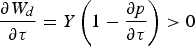
Equation (11) illustrates the rate of change in the shadow value, θ. Were the shadow value positive, the transversality condition would be violated.Footnote 9 It follows that the shadow value is negative; its long-run equilibrium level is
 $$\theta^e = -{\Delta^{\prime} \lpar Z^e\rpar \over r + k}.$$
One can interpret the joint choice of τ and F d as a variant on the theme of choosing a carbon tax for each country. As we noted above, these taxes are equal in the globally optimal plan. Starting from that point, it is apparent that D has a greater incentive to increase τ than F d . Indeed, D's incentives are to raise τ and lower F d relative to the common value associated with the global planner's solution.Footnote 10
To explore the mechanics of D's problem, we use the expression for W d in equation (3) in conjunction with the market-clearing condition on Q d to write
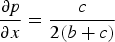
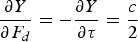
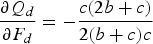
 $${\partial W_d \over \partial x} = p {\partial \lpar Q_d + Y\rpar \over \partial x} - C_d^{\prime} \lpar Q_d\rpar {\partial Q_d \over \partial x} - Y \left({\partial p \over \partial x}- {\partial \tau \over \partial x} \right)- \lpar p - \tau\rpar {\partial Y \over \partial x}\comma \;$$
for x = F d , τ. Noting that p − C d ′ (Q d ) = F d , equation (14) can be reduced to
 $${\partial W_d \over \partial x} = F_d {\partial Q_d \over \partial x} - Y {\partial p \over \partial x} + {\partial \lpar \tau Y\rpar \over \partial x}.$$
Consider two thought experiments: first, suppose that, for whatever reason, D does not or cannot impose a feed-in tariff. It then solves equation (9), constrained by τ = 0. In this scenario, τ Y = 0, and so we have:
 $${\partial W_d \over \partial F_d} = F_d {\partial Q_d \over \partial F_d} - Y {\partial p \over \partial F_d}\comma \;$$
the right-hand side of which is clearly negative. Thus, D balances the reduction in its net surplus, associated with a reduction in downstream production together with a larger import bill, against the capitalized reduction in damages, as measured by the shadow value θ. The obvious difficulty, from D's perspective, is that the reduction in Q d that follows the imposition of a domestic tax induces a price increase, which encourages U to produce more. In other words, there is some leakage associated with the domestic tax. To address this leakage, D would have an incentive to impose a feed-in tariff. Thus, D would never willingly set τ = 0.
For the second thought experiment, suppose F d = 0, so that equation (14) implies
 $${\partial W_d \over \partial \tau} = - Y {\partial p \over \partial \tau} + {\partial \lpar \tau Y\rpar \over \partial \tau}.$$
At a sufficiently large tariff level, τ
p
, imports are completely eliminated; part of this outcome may be attributed to any terms of trade effect of the tariff. Tariff revenues are nil at this level, as well as at τ = 0; for positive values less than τ
p
tariff revenues are positive. It follows that there is a positive value of the tariff τ0 at which
 ${\partial W_d \over \partial \tau} = 0$
; since D suffers damages from the carbon stock, the fact that emissions are decreasing in τ ensures that τ0 is a lower bound on D's optimal feed-in tariff.Footnote
11
There are two possible sub-cases in this second thought experiment. In the first, it is optimal for D to institute a positive domestic carbon tax. In the second, a corner solution obtains – i.e.,
 ${\partial W_d \over \partial F_d} \lt 0$
at the value τ which solves equation (10). In either event, as
 ${\partial \tau \over \partial F_d} = 0$
while
 ${\partial \tau \over \partial \tau} = 1$
, it is apparent that the two first-order conditions differ. Indeed, under the counter-factual scenario where D neglected its ability to manipulate border tax revenues by choice of feed-in tariff, including any possible terms of trade effect, the optimal arrangement would be to set the feed-in tariff at exactly the same level as the domestic carbon tax. But as D does not ignore its ability to manipulate tariff revenues it will raise τ, while lowering F
d
, relative to this counter-factual.
In the event that
 ${\partial W_d \over \partial F_d} \lt 0$
all along the optimal path for τ, the solution to D's problem reduces to one of maximizing the discounted flow of payoffs by choice of τ alone. Since this problem is simpler to analyze, we devote the remainder of this section to a discussion of this restricted problem.
3.3. Optimal tariffs in the restricted problem
For some combinations of demand and supply parameters, D's optimal choice of local tax is nil at each point in time, i.e., for all values of the feed-in tariff up to the steady-state. In this event we can recast D's non-cooperative problem as choosing τ to maximize the present discounted value of the stream of its payoffs. This variant of the problem is simpler to analyze, since there is only one control variable. For this restricted version of D's optimization problem, the current-value Hamiltonian is
 ${\cal H} = W_d \lpar \tau\rpar - \Delta \lpar Z\rpar + \theta \lsqb \phi Q\lpar \tau\rpar - kZ\rsqb $
, where the flows of net benefits and equilibrium market output are functions of τ. The necessary condition for the choice of feed-in tariff is
 $$W_{d}^{\prime} \lpar \tau\rpar = - \theta \phi Q^{\prime} \lpar \tau\rpar \semicolon \;$$
as in the unrestricted variant of the model, evolution of the shadow value is described by equation (11), and the transversality condition
 $\mathop{\lim}\limits_{t \rightarrow \infty} \theta \lpar t\rpar Z\lpar t\rpar e^{-rt} = 0$
applies.
By totally differentiating equation (15) and combining with equation (11), one can characterize the evolution of the optimal tariff as
 $${\dot{\tau} \over \tau} = {r + k - \phi \left({Q^{\prime}\lpar \tau\rpar \over W_d^{\prime} \lpar \tau\rpar } \right)\Delta^{\prime} \lpar Z\rpar \over \eta_{W_d} - \eta_Q}\comma \;$$
where
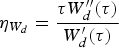 $\eta_{W_d} = {\tau W_{d}^{\prime \prime}\lpar \tau\rpar \over W_{d}^{\prime} \lpar \tau\rpar }$
is the elasticity of W
d
with respect to τ and
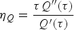 $\eta_{Q} = {\tau Q^{\prime \prime}\lpar \tau\rpar \over Q^{\prime}\lpar \tau\rpar }$
is the elasticity of Q with respect to τ. Combining this expression with the state equation, (1), and using the fact that
 $\dot{\tau} = \tau^{\prime}\lpar Z\rpar \dot{Z}$
, we obtain the feedback decision rule governing the time path of optimal feed-in tariffsFootnote
12
:
 $$\tau^{\prime}\lpar Z\rpar = {r + k - \phi \left({Q^{\prime}\lpar \tau\rpar \over W_d^{\prime} \lpar \tau\rpar } \right)\Delta^{\prime}\lpar Z\rpar \over \left(\eta_{W_d} - \eta_Q \right)\left(\phi Q\lpar \tau\rpar - kZ \right)} \tau\lpar Z\rpar.$$
This decision rule is a non-linear first-order ordinary differential equation; existence of a solution over some compact set of stocks follows from standard theorems (see, e.g., Boyce and DiPrima, Reference Boyce and DiPrima2005: 68–70).
Using the time paths of pollution and tariff, the steady state can be found as the solution of the system of two equations,
 $\dot{\tau } = 0$
and
 $\dot{Z} = 0$
:
 $${W_{d}^{\prime} \lpar \tau^e\rpar \over Q^{\prime} \lpar \tau^e\rpar } = {\phi \Delta^{\prime} \lpar Z^e\rpar \over r + k}\semicolon \;$$
 $$Z^e = \phi Q \lpar \tau^e\rpar /k.$$
The long-run equilibrium shadow price of carbon is negative and equal to
 $$\theta^e = - {\Delta^{\prime}\lpar Z^e\rpar \over r + k}.$$
It is straightforward to show that the determinant of the Jacobian matrix of the system equations (18)–(19) is negative and thus the steady state is a saddle point. Given the configuration of the
 $\dot{\tau} = 0$
and
 $\dot{Z} = 0$
isoclines, the steady state is unique.
A comparison of equations (7) and (18) is instructive. In the socially optimal solution, the difference between the marginal impact of a change in Q upon utility and cost equals the capitalized value of marginal damages from the socially optimal steady-state pollution stock; because marginal utilities are equated across countries, as are marginal costs, the difference between marginal utility and marginal cost for D equals the capitalized value of marginal damages. In D's con-cooperative solution, the ratio
 ${W_{d}^{\prime} \lpar Q_{d}\lpar \tau^{e}\rpar \rpar \over Q_{d}^{\prime}\lpar \tau^{e}\rpar }$
equals the capitalized value of marginal damages from D's privately optimal steady-state pollution stock. As the global planner's flow payoffs correspond to the sum of the two countries' payoffs, the left-hand side of equation (18) can be written as
 $$\eqalign{{W_{d}^{\prime} \lpar \tau^{e}\rpar \over Q^{\prime}\lpar \tau^{e}\rpar } &= U^{\prime}\lpar Q\lpar \tau^{e}\rpar \rpar - C^{\prime}\lpar Q\lpar \tau^{e}\rpar \rpar - {W_u^\prime \lpar \tau^e\rpar \over Q^{\prime} \lpar \tau^e\rpar } \Longleftrightarrow \cr {W_{d}^{\prime} \lpar \tau^{e}\rpar \over Q^{\prime}\lpar \tau^{e}\rpar } & \lt U^{\prime}\lpar Q\lpar \tau^{e}\rpar \rpar - C^{\prime}\lpar Q\lpar \tau^{e}\rpar \rpar \comma \; }$$
where the inequality follows from the observation that both W u and Q are decreasing in τ. Suppose, for the sake of argument, that Z e = Z*, i.e., that the steady-state pollution stocks under the global optimal plan and D's privately optimal plan were equal. In that case, the equilibrium market level of output in steady state would be identical under the two optimization plans: Q(τ e ) = Q*. But the relation (21) implies Δ′(Z e ) < (r + k)[U′(Q(τ e )) − C′(Q(τ e ))]/ϕ, which under the maintained hypothesis must equal Δ′(Z*); accordingly, Z e < Z*, a contradiction. Thus, the two plans deliver different long-run outcomes, i.e., D's privately optimal plan is second best. Intuitively, in pursuing its unilaterally optimal policy, D chooses a globally sub-optimal border tax that causes a shift in production from U to D. The shift in production is further exacerbated if any terms of trade effect occurs. Accordingly, the long-run effect of D's unilateral tax policy is to induce too much production in D and too little in U (because the equi-marginal cost principle is violated).
4. Linear-quadratic example
To further characterize the time paths of the border tax and carbon stock, we develop a simplified variant of the model, with linear-quadratic functions. Linear-quadratic models are considered to be a good approximation for more general games and are characterized by equations of motion being linear in state and control variables and objective functionals being quadratic in state and control variables. While imposing this structure facilitates algebraic computations, some of these calculations are fairly tedious; we relegate these elements of the analysis to an online appendix.
In this variant of the model, demand is linear, with intercept a
k
and slope −b
k
in country k: Q
k
d
= a
k
− b
k
p; and supply in country k is linear, with zero intercept and slope c
k
(which corresponds to assuming that marginal costs in country k are linear, with zero intercept and slope 1/c
k
). To minimize notational clutter, we focus on a stark version of this example, where slopes of demand and supply relations are equal across the two countries (b
d
= b
u
= b;c
d
= c
u
= c). For there to be trade, we require a
d
> a
u
. Finally, we assume the damage function is also quadratic:
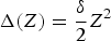 $\Delta\lpar Z\rpar = {\delta \over 2}Z^2$
, which implies linear marginal damage Δ′(Z) = δZ.
In the presence of a domestic tax in D and a border tariff, the countries' supply relations become
 $$Q_u = c \lpar p - \tau\rpar \semicolon \;$$
 $$Q_d = c \lpar p - F_d\rpar .$$
At each point in time, market clearing requires that combined quantity demanded equals combined quantity supplied: Q u d + Q d d = Q u + Q d . The resultant equilibrium price is a linear function of the domestic carbon tax and feed-in tariff:
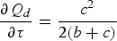
 $$p = p^0 + {c \over 2\lpar b + c\rpar } \lpar \tau + F_d\rpar \comma \;$$
where
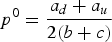 $p^{0} = {a_{d} + a_{u} \over 2\lpar b + c\rpar }$
is the equilibrium price in the absence of any taxes. Exports from U to D can be calculated as the difference between quantity demanded and quantity supplied in D, so Y = a
d
− (b + c)p + cF
d
. Alternatively, exports are equal to the difference between quantity supplied and quantity demanded in U, so Y = −a
u
+ (b + c)p − cτ. Combining these relationships yields
 $$Y = Y^0 - {c \over 2} \lpar \tau - F_d\rpar \comma \;$$
where
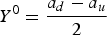 $Y^{0} = {a_{d} - a_{u} \over 2}$
is the level of exports from U to D in the absence of any taxes. Finally, the two countries' instantaneous payoff functions can be written as
 $$W_d\lpar \tau\comma \; F_d\rpar = {a_d^2 \over 2b} - {b \over 2}p^2 - {c \over 2}\lpar p - F_d\rpar ^2 - \lpar p -\tau \rpar Y - {\delta \over 2}Z^2\semicolon \;$$
 $$W_u \lpar \tau\comma \; F_d\rpar = {a_u^2 \over 2b} - {b \over 2}\lpar p - \tau\rpar ^2 - {c \over 2}\lpar p - \tau\rpar ^2 + \lpar p -\tau \rpar Y.$$
4.1. Socially optimal solution
In the globally optimal solution, the two countries' outputs are linked by the equi-marginal principle – namely, their marginal costs are equal. As the marginal cost for country k is
 ${Q_k \over c}$
, it follows that the countries' outputs are equal, and hence each produces half the global output. An immediate implication is that the tax rates levied on the countries must be equal, i.e., τ = F
d
. Using these observations, we derive the global payoff function as
 $$W = {a_d + a_u \over 2b} Q - {1 \over 4b} Q^2 + {1 \over b} \lpar Y^0\rpar ^2 - {1 \over 4c}Q^2 - {\delta \over 2} Z^2.$$
The optimal level of combined output is then given by
 $${a_u + a_d \over 2b} - {Q \over 2b} - {Q \over 2c} + \phi m = 0\comma \;$$
where m is the global shadow value of the pollution stock.
Upon differentiating the expression on the left-hand side of equation (29), one may obtain a differential equation governing combined output in the social optimal problem. Using then equation (5) to substitute for
 $\dot{m}$
, equation (29) to eliminate m, and recalling the definition of p
0, we have
 $$\dot{Q} = -2c \lpar r + k\rpar p^0 + \lpar r + k\rpar Q + {2bc\delta \phi \over b + c} Z.$$
Setting the right-hand side equal to zero leads to the
 $\dot{Q} = 0$
isocline:
 $$Q = {c\lpar a_u + a_d\rpar \over \lpar b + c\rpar } - {2bc\delta \phi \over \lpar b + c\rpar \lpar r + k\rpar } Z.$$
The state equation for Z can then be used to obtain the
 $\dot{Z} = 0$
isocline:
 $$Q = {k \over \phi} Z.$$
Combining equations (30) and (31) then produces the steady-state.
It is easy to see that this problem is saddle-point stable, and so there is a unique asymptotically stable steady state.Footnote 13 The steady-state equilibrium output and pollution stock are:
 $$Q^{\ast} = {2ck \lpar b + c\rpar \lpar r + k\rpar p^0 \over k\lpar r + k\rpar \lpar b + c\rpar + 2bc \delta \phi^2}\semicolon \;$$
 $$Z^{\ast} = {2c \lpar b + c\rpar \lpar r + k\rpar \phi p^0 \over k\lpar r + k\rpar \lpar b + c\rpar + 2bc \delta \phi^2}.$$
As we noted above, the global planner can obtain this outcome by charging all firms a pollution tax equal to the capitalized value of long-run imputed pollution stock marginal damages in this linear-quadratic framework:
 $\tau^{\ast} = {\delta \phi Z^{\ast} \over r + k}$
. Then, using equation (33), we obtain
 $$\tau^{\ast} = { 2c \lpar b + c\rpar \delta \phi^2 p^0 \over k\lpar r + k\rpar \lpar b + c\rpar + 2bc \delta \phi^2}.$$
Upon inserting the steady-state values into the two countries' payoff functions one may determine the long-run welfare levels for each country. These values can be expressed in terms of the steady-state pollution stock, or in terms of the steady-state global output; we elect to use the latter approach. The resultant values are
 $$\eqalign{W_d^{\ast} &= {a_d^2 \over 2b} - \left({b + c \over 2} \right)\lpar p^0\rpar ^2 - p^0 Y^0 + {b \phi \delta Y^0 \over \lpar b + c\rpar \lpar r + k\rpar } Z^{\ast}\cr &\quad- \left({\delta \lpar b+c\rpar \lpar r+k\rpar ^2 + b c \delta^2 \phi^2 \over 2 \lpar b + c\rpar \lpar r + k\rpar ^2} \right)\lpar Z^{\ast}\rpar ^2\semicolon \; }$$
 $$\eqalign{W_u^{\ast} &= {a_u^2 \over 2b} - \left({b + c \over 2} \right)\lpar p^0\rpar ^2 + p^0 Y^0 - {b \phi \delta Y^0 \over \lpar b + c\rpar \lpar r + k\rpar } Z^{\ast} \cr &\quad- \left({b c \delta^2 \phi^2 \over 2 \lpar b+c\rpar \lpar r + k\rpar ^2} \right)\lpar Z^{\ast}\rpar ^2.}$$
4.2. D's non-cooperative solution
Now suppose that D chooses the tax instruments so as to maximize its present discounted flow of net benefits. In an interior solution, the optimality conditions are
 $${\partial W_d \over \partial x} + \phi {\partial Q \over \partial x} \theta = 0\comma \;$$
where x = F d , τ and θ is the shadow value D places on the pollution stock. In the linear-quadratic variant we are analyzing, it is straightforward to show thatFootnote 14
 $$\eqalign{{\partial W_d \over \partial F_d} &= -p {bc \over 2\lpar b+c\rpar } - Q_d \left({c \over 2\lpar b + c\rpar } - 1 \right)- \lpar p - \tau\rpar {c \over 2} - {c \over 2\lpar b + c\rpar } Y\semicolon \; \cr {\partial W_d \over \tau} &= -p {bc \over 2\lpar b + c\rpar } - Q_d \left({c \over 2\lpar b + c\rpar } \right)+ \lpar p - \tau\rpar {c \over 2} - \left({c \over 2\lpar b + c\rpar } - 1 \right)Y.}$$
Because
 ${\partial Q \over \partial F_d} = {\partial Q \over \partial \tau}$
, the expressions on the right-hand sides of these equations must be equal in an interior solution, which implies Q
d
= c (p − τ) + Y, or
 $$\tau - F_d = {Y \over c}.$$
Combining equations (25) and (37), we deduce
 $Y = {2 \over 3} Y^0$
. Thus, if there is an interior solution, it must be the case that the border tariff is sufficiently larger than the optimal local tax so that imports are reduced by one-third. Moreover, since Y is a fixed fraction of Y
0 in this case, it must be true that the wedge between τ and F
d
is atemporal.
The optimization condition governing the feed-in tariff can be simplified to
 $$0 = {b \over b + c} Y - {bc \over 2\lpar b + c\rpar } \tau - {2bc \phi \over b + c} \theta \Longleftrightarrow \tau = {4Y^0 \over 3c} - 2 \phi \theta.$$
Thus, the
 $\dot{\tau} = 0$
isocline is described by
 $\dot{\theta} = 0$
; referring back to equation (11) and applying equation (38), this relation is given by
 $$\tau = {4Y^0 \over 3c} + {2 \delta \phi \over r + k} Z.$$
Next, combining equations (1), (22), (23), (24) and (37), one may write the
 $\dot{Z} = 0$
isocline as:
 $$Z = {2 c \phi p^0 \over k} + {2 b \phi Y^0 \over 3k\lpar b + c\rpar } - {2 b c \phi \over k\lpar b + c\rpar } \tau.$$
It is easy to see that this problem is saddle-point stable, and so there is a unique asymptotically stable steady state. In that steady state, the pollution stock is
 $$Z^{e} = \left({2\lpar r + k\rpar \lpar b + c\rpar c\phi \over k\lpar r + k\rpar \lpar b + c\rpar + 4 b c \delta\phi^2} \right)p^0 - \left({2 \lpar r + k\rpar b \phi \over k\lpar r + k\rpar \lpar b + c\rpar + 4 b c \delta \phi^2} \right)Y^0\comma \;$$
and the feed-in tariff is
 $$\tau^{e} = \left({4 \lpar b+c\rpar c \delta \phi^2 \over k\lpar r + k\rpar \lpar b + c\rpar + 4 b c \delta \phi^2} \right)p^0 + \left({k\lpar r + k\rpar \lpar b + c\rpar + b c \delta \phi^2 \over k\lpar r + k\rpar \lpar b + c\rpar + 4 b c \delta \phi^2} \right){4 \over 3c} Y^0.$$
Comparing equations (33) and (41), the long-run pollution stock is larger in the socially optimal program than in D's optimal non-cooperative plan, which suggests that the steady-state tariff must be larger in D's optimal non-cooperative program than in the socially optimal plan – an outcome that is verified by a comparison of equations (34) and (42). Moreover, it can be shown that the steady-state value of the local pollution tax is smaller than the long-run tax in the socially optimal scenario.Footnote 15
Upon substituting equations (41) and (42) into the two countries' payoff functions, one may derive the steady-state welfare levels. These are:
 $$\eqalign{W_d^e &= {a_d^2 \over 2b} - \left({b+c \over 2} \right)\lpar p^0\rpar ^2 - p^0 Y^0 + \left({7c + 16b \over 18c \lpar b+c\rpar } \right)\lpar Y^0\rpar ^2 \cr &\quad-\left({8 b c \delta^2 \phi^2 \over \lpar b + c\rpar \lpar r + k\rpar ^2} + {\delta \over 2} \right)\lpar Z^e\rpar ^2\semicolon \; }$$
 $$\eqalign{W_u^e &= {a_u^2 \over 2b} - \left({b+c \over 2} \right)\lpar p^0\rpar ^2 +\left(1 + {4b \over 3c} \right)p^0 Y^0 - \left({4b + 5c \over 18 \lpar b + c\rpar c^2} \right)\lpar Y^0\rpar ^2 \cr &\quad +\left({2b \delta \phi \over r + k} \right)\left[p^0 - \left({3c + 4b \over 3c\lpar b + c\rpar } \right)Y^0 \right]Z^e - \left({2 b^2 \delta^2 \phi^2 \over \lpar b + c\rpar \lpar r + k\rpar ^2} \right)\lpar Z^e\rpar ^2.}$$
Comparing equations (35) and (43), D can be strictly better off in the long-run under the non-cooperative regime than the cooperative regime. This result obtains because the pollution stock is smaller, and so damages are smaller, while the domestic tax is smaller and the feed-in tariff is larger than the long-run socially optimal tax. This combination steers output away from U and towards D, raising profits in D. If the combined magnitude of these effects is sufficiently large to offset the reduced consumer surplus, due to a higher price, then D's long-run welfare level is larger. By definition, the cooperative regime maximizes joint payoffs, and so U must be worse off in the non-cooperative regime.
These results pose a serious challenge to the efficacy of any joint welfare-maximizing arrangement, since such a scheme would require substantial side payments from U to D and such side payments may be politically infeasible. The observation that D may be strictly better off in the non-cooperative regime recalls a central finding by List and Mason (Reference List and Mason2001), who show that the equilibrium payoffs under an overarching regulatory authority may not dominate those obtained via the unilateral (non-cooperative) actions of a single policy maker (here, D). This outcome arises whenever there are sharp asymmetries between the two countries. In our setting, the incentives facing D and U are similarly asymmetric, inasmuch as only D suffers damages from the pollution stock. As a result, it is unclear that the two countries would be able to successfully negotiate a mutually beneficial treaty.
5. The model with local externalities
To this point the analysis has been based on the assumption that U suffers no damages from the pollutant. In this section, we investigate the implications of relaxing this assumption. To simplify the discussion, we focus on the restricted sub-case where various parameters are consistent with D choosing F d = 0 as part of its (unilateral) optimal program.
Suppose that U bears damages based on the flow of emissions created by production in U, E u (=ϕ Q).Footnote 16 To address these damages, we assume U imposes a carbon tax F u that is constrained to be non-negative.Footnote 17
For now, we retain the assumption that U does not care about climate change (and thus ignores any stock-related damages). Because the flow of emissions is determined by output, one can regard damages as implicitly being determined by Q u ; we write these as Δ u (Q u ). Thus, U's flow payoffs depend on both the output it produces (and so F u ) and D's choice of the border tax τ; U's decision problem is
 $$\eqalign{&\max_{F_u\lpar t\rpar } \vint_{0}^{\infty} e^{-rt} \lsqb W_{u} \lpar Q_{u}\comma \; \tau\rpar - \Delta_u \lpar Q_{u}\rpar \rsqb \, \hbox{dt} \cr &\hbox{subject to}\, \dot{Z} \lpar t\rpar = \phi Q - k Z\semicolon \; Z\lpar 0\rpar = Z_0\semicolon \; F_u \ge 0.}$$
As in our earlier model, production in D satisfies C
d
′ (Q
d
) = p. Production in U equates marginal cost with price less the tariff, less the carbon tax: C
u
′ (Q
u
) = p − τ− F
u
. With this in mind, U's current value Hamiltonian is
 ${\cal H}_{u} =W_{u} \lpar Q_{u} \lpar \tau\comma \; F_{u}\rpar \rpar - \Delta_u \lpar Q_{u} \lpar \tau\comma \; F_{u}\rpar \comma \; \tau\rpar + \xi \phi \lpar Q\lpar \tau\comma \; F_{u}\rpar - kZ\rpar + \psi F_{u}$
, where ξ represents the shadow price U places on the carbon stockFootnote
18
and ψ represents the LaGrangean multiplier on the non-negativity constraint for F
u
. The maximum conditions are
 $$\left({\partial W_u \over \partial Q_u} - \Delta_u^{\prime} \lpar Q_u\rpar \right){\partial Q_u \over \partial F_u} + \xi \phi {\partial Q \over \partial F_u} + \psi = 0\semicolon \;$$
 $$\dot{\xi} = \lpar r + k\rpar \xi\semicolon \;$$
with the transversality condition
 $\mathop{\lim}\limits_{t \rightarrow \infty} \xi \lpar t\rpar Z\lpar t\rpar e^{-rt} = 0$
.
The solution to equation (46) is of the form ξ(t) = ξ1
e
(r+k)t
. Unless Z goes to zero, which cannot happen if output levels are positive, the only way for the transversality condition to hold is for ξ1 = 0. But then it follows that ξ(t) = 0 for all t, i.e., U solves a sequence of static problems: at each moment, U wishes to set
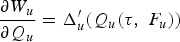 ${\partial W_{u} \over \partial Q_{u}} = \Delta_u^{\prime} \lpar Q_{u} \lpar \tau\comma \; F_{u}\rpar \rpar $
, which is just the familiar rule that marginal benefits of consumption should equal the sum of marginal production cost with marginal damage. Denote the output at which this result occurs as Q
u
*. To induce this output, U applies a local tax F
u
such that
 $$p^{\tau} - C_{u}^{\prime} \lpar Q_{u}^{\ast}\rpar = \Delta_u^{\prime} \lpar Q_{u}^{\ast}\rpar = F_u^{\ast} + \tau$$
subject to the constraint that F u ≥ 0. In other words, the sum F u * + τ is a constant.
For future reference, let
 $\hat{\tau} = \Delta_u^{\prime} \lpar Q_{u}^{\ast}\rpar $
; if
 $\tau \ge \hat{\tau}$
then F
u
* = 0, i.e.,
 $\hat{\tau}$
is the smallest feed-in tariff that would lead U to set a carbon tax equal to zero. If D sets a tariff below
 $\hat{\tau}$
, then U will choose the carbon tax
 $$F_u^{\ast} = \Delta_u^{\prime} \lpar Q_{u} \ast\rpar - \tau.$$
Because U will adjust its local tax so as to induce the output level Q
u
*, the only impact upon D's payoff from adjusting the feed-in tariff is on the revenues captured from imported production. In particular, the fact that U induces Q
u
at each point in time implies that the equilibrium price does not change if τ is varied. Since a slight increase in tariff would transfer some rents from U to D, it would never be in D's interest to set a tariff smaller than
 $\hat{\tau}$
. On the other hand, it is conceivable that D chooses a level of τ that exceeds
 $\hat{\tau}$
. At any point in time where that turns out to be the case, the outcome is as discussed in the preceding sections (amended by the inequality constraint
 $\tau \ge \hat{\tau}$
).
We therefore conclude that when U suffers flow damages, the border tax chosen by D is no smaller than the level derived in section 3. Accordingly, production in U and total emissions are no larger than in section 3, implying that the steady-state carbon stock must be no larger here. Moreover, in the event that there is a difference as compared to the scenario discussed in section 3, both players become static optimizers when U suffers flow damages. In such a circumstance, the only role ascribed to the tariff is to transfer rents from U to D. But the time path of production in U and emissions are first-best from U's perspective, in the sense that they balance marginal benefits from consumption with the marginal opportunity cost of production (which includes both marginal production costs and induced marginal damages).
We conclude this section by sketching out the problem when U does care about climate change and thus takes into account damages from the carbon stock. For expositional simplicity, we abstract from flow damages (though the extension is straightforward). In this scenario, one can write U's flow payoffs as the difference between W u and damages Δ u (Z). If U believes D's strategy depends on Z, as would occur in the Markov-perfect feedback equilibrium, then U's problem can be expressed as
 $$\eqalign{&\max_{F_u\lpar t\rpar } \vint_{0}^{\infty} e^{-rt} \left[W_{u} \lpar \tau \lpar Z\rpar \comma \; F_u\rpar -\Delta_u \lpar Z\rpar \right]\, \hbox{dt} \cr &\hbox{subject to}\, \dot{Z} \lpar t\rpar = E \lpar \tau\rpar - kZ\comma \; Z\lpar 0\rpar = Z_0\comma \; }$$
where we have combined the two players' emissions in the equation of motion for the carbon stock. U then selects a sequence of effluent taxes, given the strategy that D employs. This revision alters the equation of motion for U's shadow price of pollution changes in an important manner. Now, the evolution of the shadow price of carbon satisfies
 $$\dot{\xi} = \lpar r + k\rpar \xi + \Delta_u^{\prime} \lpar Z\rpar - \left[{\partial W_u \over \partial \tau} +\xi \phi {\partial Q \over \partial \tau} \right]\tau^{\prime} \lpar Z\rpar.$$
Since marginal damages in this scenario are non-zero, as is the third term, the solution to the differential equation on ξ is no longer an exponential. But then the transversality condition does not imply the shadow price must be nil at every point in time; it follows that U is no longer a static optimizer.
To derive the Markov-perfect feedback equilibrium, one must simultaneously solve the maximum principle for both players. That process leads to a pair of feedback strategies, τ(Z) and F u (Z). For example, U's strategy yields a value of F u that solves
 $${\partial W_u \lpar \tau \lpar Z\rpar \comma \; F_u\rpar \over \partial F_u} - \xi \phi {\partial Q \over \partial F_u} = 0.$$
For a given value of the feed-in tariff, increases in the carbon tax will lower combined output:
 ${\partial Q \over \partial F_{u}} \lt 0$
. Moreover, because the carbon stock harms U, increases in Z will lower the stream of payoffs, and so the shadow value ξ will also be negative. It follows that the optimal carbon tax yields
 ${\partial W_u \over F_u} \gt 0$
, i.e., it falls short of the value at which all marginal gains to U are realized.
To illustrate the mechanics of this analysis, we return to the linear-quadratic framework adopted in section 4, in which Markov strategies may be linear in the carbon stock:
 $$\tau \lpar Z\rpar = \tau_0 + \tau_1 Z\semicolon \;$$
 $$F_u \lpar Z\rpar = f_0 + f_1 Z.$$
Since emissions are a linear function of the feed-in tariff and carbon tax, it follows that the state equation is a linear first-order differential equation. As a result, the equilibrium path of the carbon stock is an exponential; because the carbon stock tends to its long run equilibrium (steady-state) level
 $\hat{Z}$
, the coefficient in the exponential must be negative:
 $$Z\lpar t\rpar = \lpar Z_0 - \hat{Z}\rpar \, e^{-\nu t} + \hat{Z}\comma \;$$
with ν > 0. The linear strategies in equations (50) and (51) then imply that τ and F u are exponentials as well. The intuition we sketched out above suggests that, in the long run, where the carbon tax is essentially fixed, it is in D's best interests to choose a sufficiently high feed-in tariff so as to force the carbon tax to zero. Thus, we expect that F u falls over time, ultimately to zero; at the same time, τ rises over time. Finally, with damages in U added into the analysis, the level of emissions is lower at each point in time than would be the case in the model of section 4.
6. Concluding remarks
Concerns about limiting carbon emissions have recently led some high-income countries to invoke feed-in tariffs and border tax adjustments. These instruments serve two purposes: they increase the cost of associated products in the importing country, reducing the level of consumption while boosting competing domestic production; they also increase the cost of doing business in the importing country, inducing the exporting country to adjust its behavior. Under an optimistic view of these incentives, the exporting country will limit emissions, and perhaps invoke some sort of climate policy; the potential for such adaptation is most intriguing for transitioning countries such as those found in Eastern Europe.
Recent work has suggested that border taxes are more likely to shift terms of trade, and relatively less likely to reduce carbon emissions (Weitzel et al., Reference Weitzel, Hübler and Peterson2012). Our results are somewhat less pointed in this regard (although elements of these two effects are reflected in our outcomes). In a model where the transitioning country ignores climate change and thus any possible damages, there is scope for a feed-in tariff to inhibit carbon emissions. But if the exporting country suffers damages from the flow of pollution emissions (but not stock-related damages from carbon accumulation), the major issue becomes one of trade-shifting. Lastly, if the exporting country does recognize and care about climate damages related to the carbon stock, then the imposition of feed-in tariffs or border taxes induces the exporting country to adjust its behavior, adopting a carbon tax. This is an important consideration, which goes beyond the scope of analysis in much of the extant literature.
In our view, the potential for feed-in tariffs or border tax adjustments to serve as a surrogate for internationally agreed climate policies merits serious consideration. Whether the ultimate impact is to shift trade patterns or to inhibit carbon policies, these policies could induce exporting countries to adopt some form of climate policy. This incentive may be most significant for transitioning economies, particularly those countries in Eastern Europe that are dependent on trade with their more developed Western neighbors. As our results indicate, such exporting economies may be more amenable to adapting their policies in response to carbon pricing initiated by importing countries. The practical significance of this sort of effect is of course an empirical question.
Supplementary materials and methods
The supplementary material referred to in this paper can be found online at journals.cambridge.org/EDE/.