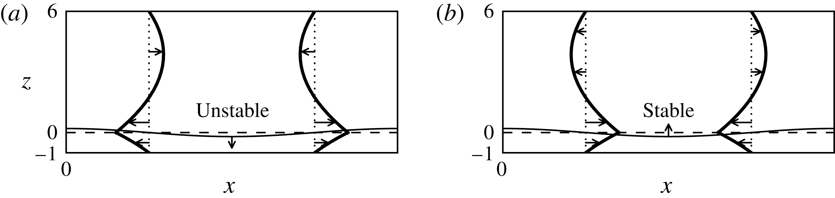
1 Introduction
Flows of fluid films occur frequently in nature and industry. (For recent reviews, see e.g. Oron, Davis & Bankoff Reference Oron, Davis and Bankoff1997; Craster & Matar Reference Craster and Matar2009.) Instabilities of multifluid film flows are of considerable interest (Joseph & Renardy Reference Joseph and Renardy1993). Such instabilities can be significantly influenced by interfacial surfactants.
Surfactants are surface active compounds that reduce the surface tension between two fluids, or between a fluid and a solid. Frenkel & Halpern (Reference Frenkel and Halpern2002) (hereafter referred to as FH) and Halpern & Frenkel (Reference Halpern and Frenkel2003) (hereafter referred to as HF) uncovered a new instability due to interfacial surfactants: certain stable surfactant-free Stokes flows become unstable if an interfacial surfactant is introduced. For this, the interfacial shear of velocity must be non-zero; in particular, this instability disappears if the basic flow is stopped. In contrast to the well-known instability of two viscous fluids (Yih Reference Yih1967) which needs inertia effects for its existence, the new instability may exist in the absence of fluid inertia. With regard to multifluid channel flows, this instability has been further studied in such papers as Blyth & Pozrikidis (Reference Blyth and Pozrikidis2004a ,Reference Blyth and Pozrikidis b ), Pozrikidis (Reference Pozrikidis2004), Frenkel & Halpern (Reference Frenkel and Halpern2005), Wei (Reference Wei2005), Frenkel & Halpern (Reference Frenkel and Halpern2006), Halpern & Frenkel (Reference Halpern and Frenkel2008), Bassom, Blyth & Papageorgiou (Reference Bassom, Blyth and Papageorgiou2010), Peng & Zhu (Reference Peng and Zhu2010), Kalogirou, Papageorgiou & Smyrlis (Reference Kalogirou, Papageorgiou and Smyrlis2012), Samanta (Reference Samanta2013), Kalogirou & Papageorgiou (Reference Kalogirou and Papageorgiou2016) and Picardo, Radhakrishna & Pushpavanam (Reference Picardo, Radhakrishna and Pushpavanam2016).
For simplicity, consideration in FH and HF was restricted to flows whose stability properties did not depend on gravity. The same is true for the further studies mentioned above. The stability effects of gravity in multifluid horizontal systems without surfactants were investigated since as long ago as the fundamental work of Lord Rayleigh (Reference Rayleigh1900). Gravity is stabilizing when the lighter fluid layer is on top of the heavier fluid layer, or destabilizing when heavier fluid is above the lighter fluid. The latter is the well-known Rayleigh–Taylor instability (RTI) that has been studied extensively (see, e.g. the classical book by Chandrasekhar Reference Chandrasekhar1961). Recent reviews of the RTI and its numerous important applications are given in Kull (Reference Kull1991). The combination of RTI with various viscous, inertial and nonlinear effects in two-fluid channel flows was studied in such papers as Babchin et al. (Reference Babchin, Frenkel, Levich and Sivashinsky1983), Hooper & Grimshaw (Reference Hooper and Grimshaw1985) and Yiantsios & Higgins (Reference Yiantsios and Higgins1988). Some industrial situations where surfactant and gravity effects are both relevant in oil recovery were studied e.g. in Hirasaki & Zhang (Reference Hirasaki and Zhang2004).
In this paper, we study the interplay between the inertialess effects due to surfactants and gravity in Couette flows of two incompressible Newtonian liquids in a horizontal channel. Both linear and nonlinear stability is investigated. One can expect a rich landscape of stability properties, especially since, even in the absence of gravity, there are two active normal modes for each wavenumber of infinitesimal disturbances, corresponding to the two interfacial functions: the interface displacement and the interfacial surfactant concentration (FH, HF). Their growth rates are given by a (complex) quadratic equation, and hence in many instances numerical results may enjoy analytic (asymptotic) corroboration. The linear stability properties of two-layer Couette flows for arbitrary wavelength with both interfacial surfactant and gravitational effects were the subject of the dissertation by Schweiger (Reference Schweiger2013), and will be further investigated elsewhere. On the other hand, the nonlinear lubrication approximation equations were obtained in Blyth & Pozrikidis (Reference Blyth and Pozrikidis2004b ) for the long-wave disturbances of these flows, although only zero gravity results were given in that paper. The linearized lubrication-approximation approach was used also in Wei (Reference Wei2005) for the no-gravity case to offer a mechanism of long-wave instability. In this paper, we re-derive, with certain modifications, the aforementioned system of two nonlinear lubrication-approximation equations coupling the interface location and the interfacial surfactant concentration for the Couette flows with the insoluble surfactant and gravity, provided that the characteristic length scale of the flow disturbances is much larger than the thicknesses of both fluid layers. The linear system of equations coupling the surfactant and gravity follows as the limit of (long) infinitesimal waves. It is also of interest to determine, to the two leading orders in the long-wave parameter, which are allowed by the lubrication approximation, the complete set of eigenfunctions of the eigenvalue problem for the normal modes including the velocities and pressures, and, based on these, to clarify the mechanisms of instability for the two normal modes. The inclusion of gravity may be expected to clarify the limitations of the conclusions obtained by studying the flow in the absence of gravity and to observe new linear and nonlinear effects.
Concerning the linear stability, in the present paper, we concentrate on the parametric thresholds of instability. The latter turn out to be determined by the leading order of the small wavenumber expansion, which allows neglecting the higher-order capillary effects. However, we include these effects in investigating the nonlinear stages of the instability. A natural question concerning the interaction of gravity and the surfactants is whether sufficiently strong gravitational forces can always suppress the linear instability caused by surfactants. On the other hand, one can ask if surfactants can suppress the Rayleigh–Taylor instability. These questions are answered below.
The nonlinear saturation of the surfactant instability was studied before for the case of one layer being infinitely thick, and it was shown that it is impossible to have the saturated amplitudes small for both surfactant and interface displacement (Frenkel & Halpern Reference Frenkel and Halpern2006). For the finite thickness ratio, the limited nonlinear simulations in Blyth & Pozrikidis (Reference Blyth and Pozrikidis2004b ) featured the same property, but the question remained if it holds in all cases. We investigate this below in a more systematic way (which shows that both surfactant disturbance and interface displacement can be small in some saturated regimes).
The paper is organized as follows. In § 2, the general stability problem is formulated. In § 3, the nonlinear and linear systems of governing equations are obtained. The long-wave growth rates and instability thresholds are considered in § 4. Also in that section, we study the surfactant-thickness and vorticity-thickness phase differences in connection with their purported significance for (in)stability. In § 5, we uncover the physical mechanisms of instability for the different branches of normal modes. Also, the eigenfunctions of the normal modes, in particular the velocities, are discussed. In § 6, the nonlinear evolution of disturbances is studied, including both weakly and strongly nonlinear regimes. Finally, § 7 contains summary, discussion and concluding remarks. Appendix A gives the complete collection of the normal-mode eigenfunctions.
2 General problem framework
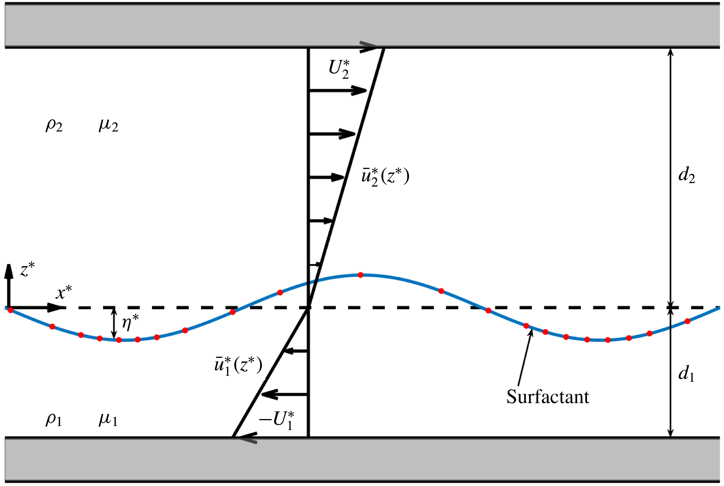
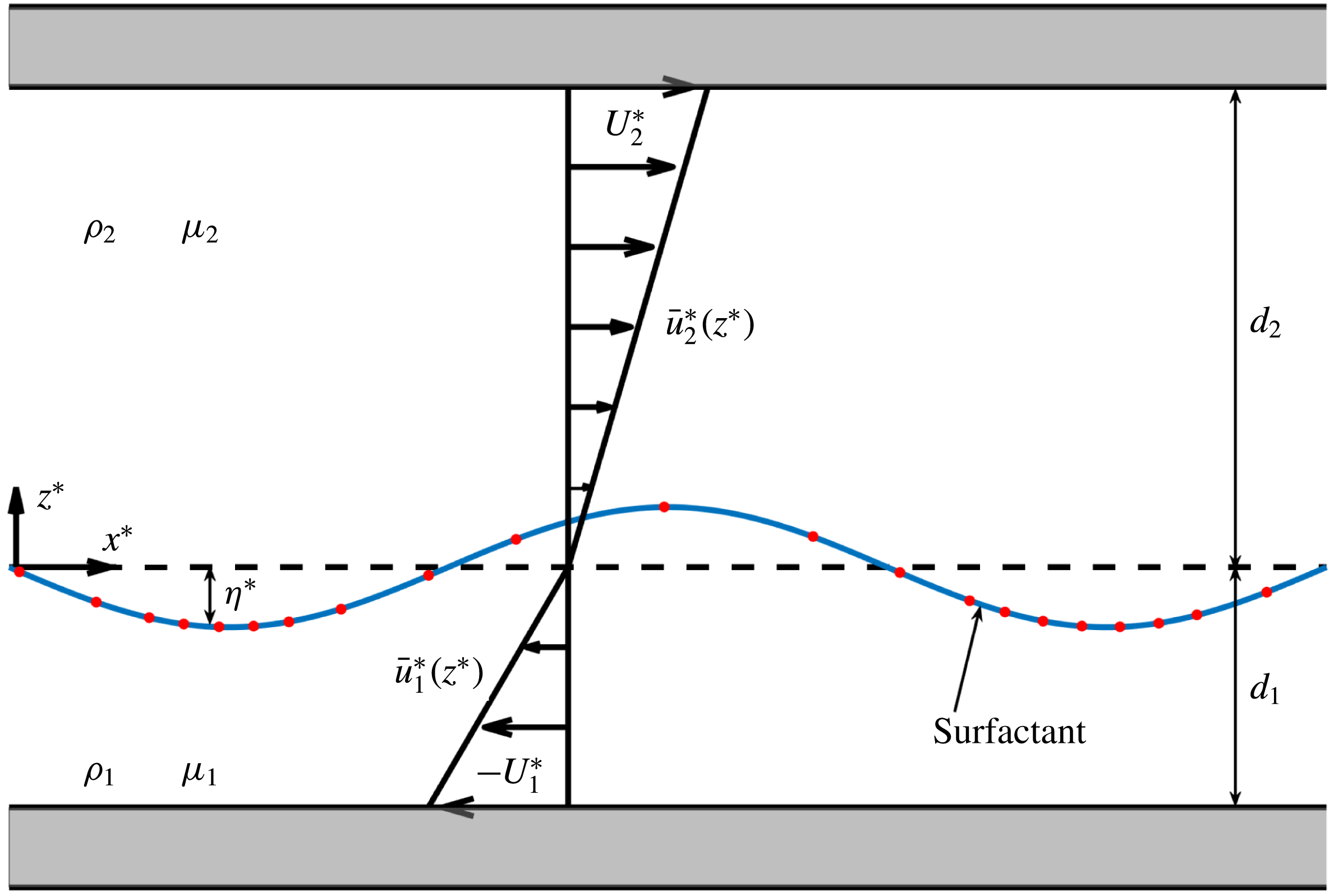
The formulation used in this paper is similar to that of HF; however, gravitational effects, which were absent in HF, play an active role here. Two immiscible fluid layers with different densities, viscosities and thicknesses are bounded by two infinite horizontal plates, a distance
 $d=d_{1}+d_{2}$
apart, with the top plate moving at a constant relative velocity
 $U^{\ast }$
, as shown in figure 1. The vertical coordinate is denoted
 $z^{\ast }$
, and we choose
 $z^{\ast }=0$
at the base liquid–liquid interface. (We use the symbol
 $^{\ast }$
to indicate a dimensional quantity.) The top plate is located at
 $z^{\ast }=d_{2}$
and the bottom plate is located at
 $z^{\ast }=-d_{1}$
. The horizontal
 $x^{\ast }$
-axis is streamwise. At the interface, the surface tension,
 $\unicode[STIX]{x1D70E}^{\ast }$
, depends on the concentration of the insoluble surfactant monolayer,
 $\unicode[STIX]{x1D6E4}^{\ast }$
. The basic flow is driven by the steady motion of the top plate. If the frame of reference is fixed at the liquid–liquid interface, the velocity of the bottom plate is denoted
 $-U_{1}^{\ast }$
, and that of the top plate is
 $U_{2}^{\ast }$
, then clearly
 $U_{1}^{\ast }+U_{2}^{\ast }=U^{\ast }$
. In the base state, the horizontal velocity profiles are linear in
 $z^{\ast }$
, the interface is flat, and the surfactant concentration is uniform. Once disturbed, the surfactant concentration,
 $\unicode[STIX]{x1D6E4}^{\ast }(t^{\ast },x^{\ast })$
, is no longer uniform, and there is a varying deflection of the interface,
 $\unicode[STIX]{x1D702}^{\ast }(t^{\ast },x^{\ast })$
, where
 $t^{\ast }$
is time.
Sketch of a disturbed two-layer Couette flow of two horizontal liquid layers with different thicknesses, viscosities and mass densities. The insoluble surfactant monolayer is located at the interface and is indicated by the dots. The (spanwise) uniform gravity field with a constant acceleration
 $g$
is not shown.
The governing equations in dimensional form for this problem are given, for example, in Frenkel & Halpern (Reference Frenkel and Halpern2016). We write the full set of them in a dimensionless form below. We use the following notations (with
 $j=1$
for the bottom liquid layer and
 $j=2$
for the top liquid layer):
 $\unicode[STIX]{x1D70C}_{j}$
is the density;
 $\boldsymbol{v}_{j}^{\ast }=(u_{j}^{\ast },w_{j}^{\ast })$
is the fluid velocity vector with horizontal component
 $u_{j}^{\ast }$
and vertical component
 $w_{j}^{\ast }$
;
 $p_{j}^{\ast }$
is the pressure;
 $\unicode[STIX]{x1D707}_{j}$
is the viscosity; and
 $g$
is the gravity acceleration.
We assume the dependence of surface tension on the surfactant concentration given by the well-known Langmuir isotherm relation (Edwards, Brenner & Wasan Reference Edwards, Brenner and Wasan1991), which becomes the linear Gibbs isotherm when the surfactant concentration
 $\unicode[STIX]{x1D6E4}^{\ast }$
is much smaller than the maximum packing value
 $\unicode[STIX]{x1D6E4}_{\infty }$
. Then we can write
 $$\begin{eqnarray}\unicode[STIX]{x1D70E}^{\ast }=\unicode[STIX]{x1D70E}_{0}-RT(\unicode[STIX]{x1D6E4}^{\ast }-\unicode[STIX]{x1D6E4}_{0}),\end{eqnarray}$$
where
 $\unicode[STIX]{x1D70E}_{0}$
is the base surface tension corresponding to the base surfactant concentration
 $\unicode[STIX]{x1D6E4}_{0}$
,
 $R$
is the universal gas constant and
 $T$
is the absolute temperature.
We introduce the following dimensionless variables:
 $$\begin{eqnarray}\left.\begin{array}{@{}c@{}}(x,z,\unicode[STIX]{x1D702})={\displaystyle \frac{(x^{\ast },z^{\ast },\unicode[STIX]{x1D702}^{\ast })}{d_{1}}},\quad t={\displaystyle \frac{t^{\ast }}{d_{1}\unicode[STIX]{x1D707}_{1}/\unicode[STIX]{x1D70E}_{0}}},\quad \boldsymbol{v}_{j}=(u_{j},w_{j})={\displaystyle \frac{(u_{j}^{\ast },w_{j}^{\ast })}{\unicode[STIX]{x1D70E}_{0}/\unicode[STIX]{x1D707}_{1}}},\\ p_{j}={\displaystyle \frac{p_{j}^{\ast }}{\unicode[STIX]{x1D70E}_{0}/d_{1}}},\quad \unicode[STIX]{x1D6E4}={\displaystyle \frac{\unicode[STIX]{x1D6E4}^{\ast }}{\unicode[STIX]{x1D6E4}_{0}}},\quad \unicode[STIX]{x1D70E}={\displaystyle \frac{\unicode[STIX]{x1D70E}^{\ast }}{\unicode[STIX]{x1D70E}_{0}}}.\end{array}\right\}\end{eqnarray}$$
(Similar to FH and HF, using the velocity scale
 $\unicode[STIX]{x1D70E}_{0}/\unicode[STIX]{x1D707}_{1}$
, rather than the plate speed, allows one to include into consideration the case of zero plate velocity corresponding to the absence of base flow.) The continuity equation and the Navier–Stokes momentum equations are, respectively,
 $$\begin{eqnarray}\displaystyle & \unicode[STIX]{x1D735}\boldsymbol{\cdot }\boldsymbol{v}_{j}=0, & \displaystyle\end{eqnarray}$$
 $$\begin{eqnarray}\displaystyle & \displaystyle \frac{Re_{j}}{Ca_{j}}\left(\frac{\unicode[STIX]{x2202}\boldsymbol{v}_{j}}{\unicode[STIX]{x2202}t}+\boldsymbol{v}_{j}\boldsymbol{\cdot }\unicode[STIX]{x1D735}\boldsymbol{v}_{j}\right)=-\unicode[STIX]{x1D735}p_{j}+m_{j}\unicode[STIX]{x1D6FB}^{2}\boldsymbol{v}_{j}-Bo_{j}\hat{\boldsymbol{z}}, & \displaystyle\end{eqnarray}$$
where the vector operator
 $\unicode[STIX]{x1D735}:=(\unicode[STIX]{x2202}/\unicode[STIX]{x2202}x,\unicode[STIX]{x2202}/\unicode[STIX]{x2202}z)$
,
 $Re_{j}:=U_{j}^{\ast }d_{1}/\unicode[STIX]{x1D707}_{1}$
is the Reynolds number,
 $Ca_{j}:=U_{j}^{\ast }\unicode[STIX]{x1D707}_{1}/\unicode[STIX]{x1D70E}_{0}$
is the capillary number,
 $m_{j}:=\unicode[STIX]{x1D707}_{j}/\unicode[STIX]{x1D707}_{1}$
– where from
 $m_{1}=1$
and
 $m_{2}=\unicode[STIX]{x1D707}_{2}/\unicode[STIX]{x1D707}_{1}=:m$
is the viscosity ratio,
 $Bo_{j}:=\unicode[STIX]{x1D70C}_{j}gd_{1}^{2}/\unicode[STIX]{x1D70E}_{0}$
is the layer Bond number and
 $\hat{\boldsymbol{z}}$
is the unit vector of the
 $z$
-axis. The plate boundary conditions are
 $$\begin{eqnarray}u_{1}(-1)=-Ca_{1},\quad w_{1}(-1)=0,\quad u_{2}(n)=Ca_{2},\quad w_{2}(n)=0,\end{eqnarray}$$
where
 $n=d_{2}/d_{1}$
is the thickness ratio of the liquid layers. Without loss of generality, by appropriately directing the
 $z$
-axis, we obtain
 $n\geqslant 1$
. Note that this allows for negative as well as positive values of
 $g$
. The interfacial conditions for the velocities, the tangential stresses and the normal stresses are, respectively,
 $$\begin{eqnarray}\displaystyle & [\boldsymbol{v}]_{1}^{2}=0, & \displaystyle\end{eqnarray}$$
 $$\begin{eqnarray}\displaystyle & \displaystyle \frac{1}{1+\unicode[STIX]{x1D702}_{x}^{2}}\left[(1-\unicode[STIX]{x1D702}_{x}^{2})\frac{\unicode[STIX]{x1D707}}{\unicode[STIX]{x1D707}_{1}}(u_{z}+w_{x})+2\unicode[STIX]{x1D702}_{x}\frac{\unicode[STIX]{x1D707}}{\unicode[STIX]{x1D707}_{1}}(w_{z}-u_{x})\right]_{1}^{2}=-\frac{\unicode[STIX]{x1D70E}_{x}}{(1+\unicode[STIX]{x1D702}_{x}^{2})^{1/2}}, & \displaystyle\end{eqnarray}$$
and
 $$\begin{eqnarray}\left[(1+\unicode[STIX]{x1D702}_{x}^{2})p-2\frac{\unicode[STIX]{x1D707}}{\unicode[STIX]{x1D707}_{1}}(\unicode[STIX]{x1D702}_{x}^{2}u_{x}-\unicode[STIX]{x1D702}_{x}(u_{z}+w_{x})+w_{z})\right]_{1}^{2}=\frac{\unicode[STIX]{x1D702}_{xx}}{(1+\unicode[STIX]{x1D702}_{x}^{2})^{1/2}}\unicode[STIX]{x1D70E},\end{eqnarray}$$
where
 $[A]_{1}^{2}=A_{2}-A_{1}$
denotes the jump in
 $A$
across the interface
 $z=\unicode[STIX]{x1D702}(t,x)$
. The surfactant transport equation is (see HF)
 $$\begin{eqnarray}\frac{\unicode[STIX]{x2202}}{\unicode[STIX]{x2202}t}(H\unicode[STIX]{x1D6E4})+\frac{\unicode[STIX]{x2202}}{\unicode[STIX]{x2202}x}(H\unicode[STIX]{x1D6E4}u)=\frac{1}{Pe}\frac{\unicode[STIX]{x2202}}{\unicode[STIX]{x2202}x}\left(\frac{1}{H}\frac{\unicode[STIX]{x2202}\unicode[STIX]{x1D6E4}}{\unicode[STIX]{x2202}x}\right),\end{eqnarray}$$
where
 $H=(1+\unicode[STIX]{x1D702}_{x}^{2})^{1/2}$
,
 $u=u(t,x,\unicode[STIX]{x1D702}(t,x))$
and
 $Pe^{-1}$
 $=D_{\unicode[STIX]{x1D6E4}}\unicode[STIX]{x1D707}_{1}/\unicode[STIX]{x1D70E}_{0}d_{1}$
is the inverse surface Péclet number, the dimensionless representation of the surface molecular diffusivity
 $D_{\unicode[STIX]{x1D6E4}}$
of the insoluble surfactant. Usually, the latter is small and the surfactant diffusion term is negligible. The kinematic boundary condition is
 $$\begin{eqnarray}\unicode[STIX]{x1D702}_{t}=w-u\unicode[STIX]{x1D702}_{x},\end{eqnarray}$$
and the dimensionless form of the equation of state for the surface tension, equation (2.1), is
 $$\begin{eqnarray}\unicode[STIX]{x1D70E}=1-Ma(\unicode[STIX]{x1D6E4}-1),\end{eqnarray}$$
where
 $Ma:=RT\unicode[STIX]{x1D6E4}_{0}/\unicode[STIX]{x1D70E}_{0}$
is the Marangoni number. It is easy to see that the Marangoni number can be written as
 $Ma=(\unicode[STIX]{x1D70E}_{c}-\unicode[STIX]{x1D70E}_{0})/\unicode[STIX]{x1D70E}_{0}$
, where
 $\unicode[STIX]{x1D70E}_{c}$
is the surface tension in the absence of surfactant. Usually
 $\unicode[STIX]{x1D70E}_{c}-\unicode[STIX]{x1D70E}_{0}\ll \unicode[STIX]{x1D70E}_{0}$
since we are restricted to the linear part of the isotherm (see, for e.g. Mensire et al. (Reference Mensire, Wexler, Guibaud, Lorenceau and Stone2016, figure 2)). This implies the range of Marangoni numbers to be
 $$\begin{eqnarray}0<Ma\ll 1.\end{eqnarray}$$
The dimensionless velocity field of the basic Couette flow, with a flat interface,
 $\unicode[STIX]{x1D702}=0$
, uniform surface tension,
 $\bar{\unicode[STIX]{x1D70E}}=1$
, and corresponding surfactant concentration,
 $\bar{\unicode[STIX]{x1D6E4}}=1$
(where the overbar indicates a base quantity), is
 $$\begin{eqnarray}\bar{u}_{1}(z)=sz,\quad \bar{w}_{1}=0,\quad \text{and}\quad \bar{p}_{1}=-Bo_{1}z\quad \text{for }-\!1\leqslant z\leqslant 0,\end{eqnarray}$$
 $$\begin{eqnarray}\bar{u_{2}}(z)=\frac{s}{m}z,\quad \bar{w}_{2}=0,\quad \text{and}\quad \bar{p}_{2}=-Bo_{2}z\quad \text{for }0\leqslant z\leqslant n.\end{eqnarray}$$
The constant
 $s$
is used to characterize the flow in place of the relative velocity of the plates, and represents the base interfacial shear rate of the bottom layer,
 $s=D\bar{u}_{1}(0)$
, where
 $D=\text{d}/\text{d}z$
. Clearly,
 $s=Ca_{1}$
, while
 $Ca_{2}=sn/m$
, and thus
 $\unicode[STIX]{x1D707}_{1}U^{\ast }/\unicode[STIX]{x1D70E}_{0}=s(1+n/m)$
. To estimate the range of
 $s$
, note that for
 $\unicode[STIX]{x1D70E}_{0}\sim 10$
(in cgs units), fairly large viscosity
 $\unicode[STIX]{x1D707}_{1}\sim 10$
and
 $U_{1}^{\ast }\sim 1$
, we obtain
 $s\sim 1$
. This implies that in practice
 $$\begin{eqnarray}0\leqslant s\leqslant 1.\end{eqnarray}$$
The disturbed state with small deviations (indicated by the top tilde,
 $^{{\sim}}$
) from the base flow is given by
 $$\begin{eqnarray}\unicode[STIX]{x1D702}=\tilde{\unicode[STIX]{x1D702}},\quad u_{j}=\bar{u}_{j}+\tilde{u} _{j},\quad w_{j}=\tilde{w}_{j},\quad p_{j}=\bar{p}_{j}+\tilde{p}_{j},\quad \unicode[STIX]{x1D6E4}=\bar{\unicode[STIX]{x1D6E4}}+\tilde{\unicode[STIX]{x1D6E4}}.\end{eqnarray}$$
3 Lubrication approximation
We will use the lubrication approximation, assuming that the characteristic horizontal length scale
 $L$
of the disturbances is much larger than the thicknesses of both layers. The equations were derived before in Blyth & Pozrikidis (Reference Blyth and Pozrikidis2004b
) for an inclined channel. We find it convenient to briefly re-derive them for our horizontal channel case and somewhat different coordinate and non-dimensionalization choices.
It is well known that in this approximation the pressure disturbances are independent of the vertical coordinate, and the horizontal velocities satisfy the second-order differential equation
 $$\begin{eqnarray}D^{2}u_{j}=\frac{1}{m_{j}}p_{jx},\end{eqnarray}$$
where we have dropped the tildes in the notations for the disturbances (for the sake of brevity). (As will become clear later, this equation combines the orders
 $1/L$
and
 $1/L^{2}$
(corresponding to its real and imaginary parts) relative to the interface displacement
 $\unicode[STIX]{x1D702}$
(see appendix A).) The general solution satisfying the no-slip conditions at the plates is
 $$\begin{eqnarray}u_{j}=\frac{1}{2m_{j}}p_{jx}(z^{2}-n_{j}^{2})+A_{j}(z-n_{j}),\end{eqnarray}$$
where the functions
 $A_{j}$
are independent of
 $z$
and may be interpreted as vorticity components; they will be determined later on. In this formula and below, by definition,
 $n_{j}$
has the values
 $n_{1}=-1$
and
 $n_{2}=n$
. The vertical velocity disturbance is determined by the continuity equation (2.3),
 $$\begin{eqnarray}Dw_{j}=-u_{jx}.\end{eqnarray}$$
The general solutions satisfying the zero velocity conditions at the plates are then
 $$\begin{eqnarray}w_{j}=\frac{1}{6m_{j}}(-z^{3}+3n_{j}^{2}z-2n_{j}^{3})p_{jxx}-\frac{1}{2}(z-n_{j})^{2}A_{jx}.\end{eqnarray}$$
The normal stress condition (2.8) yields
 $$\begin{eqnarray}\unicode[STIX]{x1D6F1}[\unicode[STIX]{x1D702},\unicode[STIX]{x1D6E4}]:=p_{1}-p_{2}=Bo\unicode[STIX]{x1D702}-\unicode[STIX]{x1D70E}\unicode[STIX]{x1D702}_{xx},\end{eqnarray}$$
where
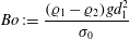 $$\begin{eqnarray}Bo:=\frac{(\unicode[STIX]{x1D71A}_{1}-\unicode[STIX]{x1D71A}_{2})gd_{1}^{2}}{\unicode[STIX]{x1D70E}_{0}}\end{eqnarray}$$
is the Bond number (equal to the difference of the Bond numbers of the layers,
 $Bo_{1}-Bo_{2}$
), and we write
 $\unicode[STIX]{x1D70E}$
in the form
 $\unicode[STIX]{x1D70E}=1-Ma\unicode[STIX]{x1D6E4}$
, where
 $\unicode[STIX]{x1D6E4}:=\tilde{\unicode[STIX]{x1D6E4}}$
, the disturbance of the surfactant concentration. Note that clearly a positive
 $Bo$
corresponds to a gravity force acting in the direction from the lighter to the heavier fluid, and the negative
 $Bo$
corresponds to the opposite direction of the gravity forces. In the latter configuration, gravity has a destabilizing effect corresponding to the Rayleigh–Taylor instability. To estimate the range of the Bond number, for the Earth’s gravity,
 $g\approx 10^{3}$
(in cgs units),
 $\unicode[STIX]{x1D70C}_{1}\sim \unicode[STIX]{x1D70C}_{2}\sim 1$
,
 $\unicode[STIX]{x1D70E}_{0}\sim 10$
, we obtain
 $|Bo|\sim 10^{2}$
for
 $d_{1}\sim 1$
and
 $Bo\sim 1$
for
 $d_{1}\sim 10^{-1}$
. Also,
 $Bo\ll 1$
for small density contrasts,
 $|\unicode[STIX]{x1D70C}_{1}-\unicode[STIX]{x1D70C}_{2}|\ll 1$
, or even for
 $|\unicode[STIX]{x1D70C}_{1}-\unicode[STIX]{x1D70C}_{2}|\sim 1$
under microgravity conditions. (Note that although
 $\unicode[STIX]{x1D702}_{xx}\sim \unicode[STIX]{x1D702}/L^{2}$
where
 $L$
is assumed large, the two terms of (3.5) are comparable for
 $Bo/\unicode[STIX]{x1D70E}$
of the order
 $1/L^{2}$
. In fact, we find below in § 6 that in the nonlinear evolution, the length scale
 $L$
might develop to be
 $L=O(\sqrt{\unicode[STIX]{x1D70E}/Bo})$
or, since
 $\unicode[STIX]{x1D70E}\approx 1$
, in view of (2.11)–(2.12), with
 $|\unicode[STIX]{x1D6E4}-1|=O(1)$
or smaller,
 $L=O(Bo^{-1/2})$
(see, e.g. the discussion in § 6.1, between equations (6.4) and (6.5)).) The tangential stress condition (2.7) yields
 $$\begin{eqnarray}Du_{1}-mDu_{2}(=\unicode[STIX]{x1D70E}_{x})=-Ma\unicode[STIX]{x1D6E4}_{x}.\end{eqnarray}$$
Hence we can eliminate
 $p_{2x}$
and
 $A_{2}\!:$
 $$\begin{eqnarray}\displaystyle & p_{2x}=p_{1x}-\unicode[STIX]{x1D6F1}_{x}, & \displaystyle\end{eqnarray}$$
 $$\begin{eqnarray}\displaystyle & \displaystyle A_{2}=\frac{1}{m}(A_{1}+Ma\unicode[STIX]{x1D6E4}_{x}+\unicode[STIX]{x1D6F1}_{x}\unicode[STIX]{x1D702}). & \displaystyle\end{eqnarray}$$
We substitute these into the expressions for
 $u_{2}$
and
 $w_{2}$
, and apply the continuity of velocity conditions, equation (2.6), at the interface
 $z=\unicode[STIX]{x1D702}$
, that is,
 $\bar{u}_{1}+u_{1}=\bar{u}_{2}+u_{2}$
, or
 $$\begin{eqnarray}u_{2}-u_{1}=\frac{m-1}{m}s\unicode[STIX]{x1D702},\end{eqnarray}$$
and
 $$\begin{eqnarray}w_{1}=w_{2}\end{eqnarray}$$
to obtain the following system of equations for
 $p_{1x}$
and
 $A_{1}$
:
 $$\begin{eqnarray}\displaystyle & & \displaystyle (-m+n^{2}+(m-1)\unicode[STIX]{x1D702}^{2})p_{1x}+2(m+n+(m-1)\unicode[STIX]{x1D702})A_{1}\nonumber\\ \displaystyle & & \displaystyle \quad =-2(m-1)s\unicode[STIX]{x1D702}+2(-n+\unicode[STIX]{x1D702})Ma\unicode[STIX]{x1D6E4}_{x}+(-n+\unicode[STIX]{x1D702})^{2}\unicode[STIX]{x1D6F1}_{x}\end{eqnarray}$$
and
 $$\begin{eqnarray}\displaystyle & & \displaystyle (2(m+n^{3})+3(m-n^{2})\unicode[STIX]{x1D702}-(m-1)\unicode[STIX]{x1D702}^{3})p_{1x}+3(-m+n^{2}-2(m+n)\unicode[STIX]{x1D702}-(m-1)\unicode[STIX]{x1D702}^{2})A_{1}\nonumber\\ \displaystyle & & \displaystyle \quad =3(m-1)s\unicode[STIX]{x1D702}^{2}-3(-n+\unicode[STIX]{x1D702})^{2}Ma\unicode[STIX]{x1D6E4}_{x}-2(-n+\unicode[STIX]{x1D702})^{3}\unicode[STIX]{x1D6F1}_{x}+C(t).\end{eqnarray}$$
Note that the second equation contains an arbitrary function
 $C(t)$
that does not depend on
 $x$
, obtained by integrating (3.11) which contains the derivatives
 $p_{1xx}$
and
 $A_{1x}$
. Solving this linear system, we can express
 $p_{1x}$
and
 $A_{1}$
, and therefore all the velocities, in terms of
 $\unicode[STIX]{x1D702}$
,
 $\unicode[STIX]{x1D6E4}$
,
 $\unicode[STIX]{x1D6F1}[\unicode[STIX]{x1D702},\unicode[STIX]{x1D6E4}]$
and
 $C(t)$
:
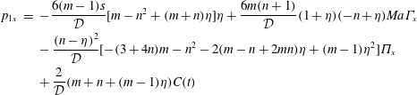 $$\begin{eqnarray}\displaystyle p_{1x} & = & \displaystyle -\frac{6(m-1)s}{{\mathcal{D}}}[m-n^{2}+(m+n)\unicode[STIX]{x1D702}]\unicode[STIX]{x1D702}+\frac{6m(n+1)}{{\mathcal{D}}}(1+\unicode[STIX]{x1D702})(-n+\unicode[STIX]{x1D702})Ma\unicode[STIX]{x1D6E4}_{x}\nonumber\\ \displaystyle & & \displaystyle -\,\frac{(n-\unicode[STIX]{x1D702})^{2}}{{\mathcal{D}}}[-(3+4n)m-n^{2}-2(m-n+2mn)\unicode[STIX]{x1D702}+(m-1)\unicode[STIX]{x1D702}^{2}]\unicode[STIX]{x1D6F1}_{x}\nonumber\\ \displaystyle & & \displaystyle +\,\frac{2}{{\mathcal{D}}}(m+n+(m-1)\unicode[STIX]{x1D702})C(t)\end{eqnarray}$$
and
 $$\begin{eqnarray}\displaystyle A_{1} & = & \displaystyle -\frac{(m-1)s}{{\mathcal{D}}}\unicode[STIX]{x1D702}[4(m+n^{3})+3(m-n^{2})\unicode[STIX]{x1D702}+(m-1)\unicode[STIX]{x1D702}^{3}]\nonumber\\ \displaystyle & & \displaystyle +\,\frac{(\unicode[STIX]{x1D702}-n)}{{\mathcal{D}}}[(4+3n)m+n^{3}+3(m-n^{2})\unicode[STIX]{x1D702}-3(m-1)n\unicode[STIX]{x1D702}^{2}+(m-1)\unicode[STIX]{x1D702}^{3}]Ma\unicode[STIX]{x1D6E4}_{x}\nonumber\\ \displaystyle & & \displaystyle +\,\frac{(\unicode[STIX]{x1D702}-n)^{2}}{{\mathcal{D}}}[2m(n+1)+(m-n^{2})\unicode[STIX]{x1D702}-2(m-1)n\unicode[STIX]{x1D702}^{2}+(m-1)\unicode[STIX]{x1D702}^{3}]\unicode[STIX]{x1D6F1}_{x}\nonumber\\ \displaystyle & & \displaystyle -\,\frac{(-(m-n^{2})+(m-1)\unicode[STIX]{x1D702}^{2})}{{\mathcal{D}}}C(t).\end{eqnarray}$$
Here the determinant
 ${\mathcal{D}}$
is
 $$\begin{eqnarray}{\mathcal{D}}=(m-1)^{2}\unicode[STIX]{x1D702}^{4}+4(m-1)(m+n)\unicode[STIX]{x1D702}^{3}+6(m-1)(m-n^{2})\unicode[STIX]{x1D702}^{2}+4(m-1)(m+n^{3})\unicode[STIX]{x1D702}+\unicode[STIX]{x1D713},\end{eqnarray}$$
where constants
 $\unicode[STIX]{x1D719}$
and
 $\unicode[STIX]{x1D713}$
are defined as follows:
 $$\begin{eqnarray}\unicode[STIX]{x1D711}=n^{3}+3n^{2}+3mn+m\end{eqnarray}$$
and
 $$\begin{eqnarray}\unicode[STIX]{x1D713}=n^{4}+4mn^{3}+6mn^{2}+4mn+m^{2}.\end{eqnarray}$$
The function
 $C(t)$
is obtained by the boundary conditions in
 $x$
. We adopt the condition of periodicity of pressure over the
 $x-$
interval of length
 $\unicode[STIX]{x1D6EC}$
similar to Blyth & Pozrikidis (Reference Blyth and Pozrikidis2004b
). (The periodic boundary conditions pertain to closed flows such as the Couette flow in a circular toroidal channel with a rectangular cross-section of Barthelet, Charru & Fabre (Reference Barthelet, Charru and Fabre1995). For rectilinear channels, we expect solutions which are largely independent of the boundary conditions at the channel ends if the channel is sufficiently long.) Then
 $$\begin{eqnarray}\int _{0}^{\unicode[STIX]{x1D6EC}}p_{1x}\,\text{d}x=0.\end{eqnarray}$$
From this equation one obtains an explicit expression for
 $C(t)$
in terms of the integrals over that interval. Thus,
 $C(t)$
is a functional of
 $\unicode[STIX]{x1D702}$
and
 $\unicode[STIX]{x1D6E4}$
.
To obtain the evolution equations, we substitute the velocity field, (3.2) and (3.4), into the kinematic boundary condition (2.10) and the surfactant transport equation (2.9):
 $$\begin{eqnarray}\displaystyle & \displaystyle \unicode[STIX]{x1D702}_{t}+\left[\frac{s}{2}\unicode[STIX]{x1D702}^{2}+\frac{1}{2}(1+\unicode[STIX]{x1D702})^{2}\left(-\frac{1}{3}(2-\unicode[STIX]{x1D702})p_{1x}+A_{1}\right)\right]_{x}=0, & \displaystyle\end{eqnarray}$$
 $$\begin{eqnarray}\displaystyle & \displaystyle \unicode[STIX]{x1D6E4}_{t}+\left[\left(s\unicode[STIX]{x1D702}-\frac{1}{2}(1-\unicode[STIX]{x1D702}^{2})p_{1x}+(1+\unicode[STIX]{x1D702})A_{1}\right)(1+\unicode[STIX]{x1D6E4})\right]_{x}=0, & \displaystyle\end{eqnarray}$$
where
 $p_{1x}$
and
 $A_{1}$
are given by (3.14) and (3.15) respectively, and we have omitted the tilde from the disturbance of surfactant. We will solve this system of strongly nonlinear evolution equations, (3.20) and (3.21), numerically, when we discuss nonlinear results in § 6.
The regimes in which
 $\unicode[STIX]{x1D702}$
and
 $\unicode[STIX]{x1D6E4}$
are much smaller than unity may be described by weakly nonlinear equations which are obtained from (3.20) and (3.21) by neglecting those nonlinear terms which are clearly smaller than some other terms:
 $$\begin{eqnarray}\displaystyle & & \displaystyle \unicode[STIX]{x1D702}_{t}+sN_{1}\unicode[STIX]{x1D702}\unicode[STIX]{x1D702}_{x}-\frac{2(m-1)n^{2}(n+1)s}{\unicode[STIX]{x1D713}}\unicode[STIX]{x1D702}_{x}-\frac{(m+n)n^{3}Bo}{3\unicode[STIX]{x1D713}}\unicode[STIX]{x1D702}_{xx}\nonumber\\ \displaystyle & & \displaystyle \quad +\,\frac{(m+n)n^{3}}{3\unicode[STIX]{x1D713}}\unicode[STIX]{x1D702}_{xxxx}+\frac{n^{2}(m-n^{2})Ma}{2\unicode[STIX]{x1D713}}\unicode[STIX]{x1D6E4}_{xx}=0\end{eqnarray}$$
and
 $$\begin{eqnarray}\displaystyle & & \displaystyle \unicode[STIX]{x1D6E4}_{t}+sN_{2}\unicode[STIX]{x1D702}\unicode[STIX]{x1D702}_{x}+\frac{(n+1)\unicode[STIX]{x1D719}s}{\unicode[STIX]{x1D713}}\unicode[STIX]{x1D702}_{x}-\frac{n^{2}(n^{2}-m)Bo}{2\unicode[STIX]{x1D713}}\unicode[STIX]{x1D702}_{xx}+\frac{n^{2}(n^{2}-m)}{2\unicode[STIX]{x1D713}}\unicode[STIX]{x1D702}_{xxxx}\nonumber\\ \displaystyle & & \displaystyle \quad -\,\frac{n(m+n^{3})Ma}{\unicode[STIX]{x1D713}}\unicode[STIX]{x1D6E4}_{xx}=0,\end{eqnarray}$$
where
 $$\begin{eqnarray}\displaystyle \left.\begin{array}{@{}c@{}}N_{1}=1+{\displaystyle \frac{(m-1)}{\unicode[STIX]{x1D713}}}[-m+4n-3n^{2}-8n^{3}]+\left[{\displaystyle \frac{4(m-1)n}{\unicode[STIX]{x1D713}}}\right]^{2}(m+n^{3})(n+1),\\ N_{2}={\displaystyle \frac{2(m-1)}{\unicode[STIX]{x1D713}}}[3n(n+1)-4(m+n^{3})]+8\left[{\displaystyle \frac{(m-1)}{\unicode[STIX]{x1D713}}}\right]^{2}(m+n^{3})(m+3n^{2}+4n^{3}).\end{array}\right\} & & \displaystyle \nonumber\\ \displaystyle & & \displaystyle\end{eqnarray}$$
We need to keep the nonlinear term in (3.22). Even though it appears that it can be neglected as compared to the term with the linear term
 $\unicode[STIX]{x1D702}_{x}$
, the latter will be eliminated by a coordinate change,
 $x\rightarrow x+Vt$
where
 $V$
is the coefficient of
 $\unicode[STIX]{x1D702}_{x}$
in (3.22). However, we will discard the nonlinear term from (3.23), since in the latter the larger (by a factor
 $1/\unicode[STIX]{x1D702}$
) linear
 $\unicode[STIX]{x1D702}_{x}$
term is not eliminated by this coordinate change. Also, calculating
 $C(t)$
(from the spatial periodicity of the pressure; see the paragraph that follows equation (3.18)), one finds that
 $C(t)$
is proportional to the average of
 $\unicode[STIX]{x1D702}^{2}$
. (Actually, it is not difficult to see that in the limit of very long channels the same conclusion holds for other boundary conditions with the end-point data being arbitrary but bounded functions of time.) So, its contribution in (3.20) and (3.21) for small
 $\unicode[STIX]{x1D702}$
and
 $\unicode[STIX]{x1D6E4}$
is at most of the orders
 $\unicode[STIX]{x1D702}^{2}\unicode[STIX]{x1D702}_{x}$
and
 $\unicode[STIX]{x1D702}^{2}\unicode[STIX]{x1D6E4}_{x}$
, and therefore is neglected in the system (3.22)–(3.23) in comparison with the nonlinear terms. These weakly nonlinear evolution equations do not imply any restrictions on the parameters beyond the lubrication approximation, and in this regard are different from the equations of Frenkel & Halpern (Reference Frenkel and Halpern2006), Bassom et al. (Reference Bassom, Blyth and Papageorgiou2010) and Kalogirou et al. (Reference Kalogirou, Papageorgiou and Smyrlis2012), which assumed a small aspect ratio
 $1/n$
(and in some cases other restrictions on the parameters). In particular, in those papers the lubrication approximation was used for the thin layer only.
We remind the reader that in view of our derivation, it is clear that the system of (3.22)–(3.23) allows for relative errors of the order
 $O(1/L^{2})$
, where
 $L$
is the characteristic length scale of solutions which is assumed to be large. The same is true of the strongly nonlinear system (3.20)–(3.21).
Below, we encounter weakly nonlinear regimes in which saturated
 $\unicode[STIX]{x1D702}$
is small but
 $\unicode[STIX]{x1D6E4}$
is not small. Then, from (3.21) we see that a nonlinear term of the form
 $N_{3}s(\unicode[STIX]{x1D702}\unicode[STIX]{x1D6E4})_{x}$
, should be added into the transport equation (3.23) where
 $$\begin{eqnarray}N_{3}=\frac{(n+1)\unicode[STIX]{x1D719}}{\unicode[STIX]{x1D713}},\end{eqnarray}$$
the coefficient of
 $\unicode[STIX]{x1D702}_{x}$
in (3.23).
From the system (3.22) and (3.23), we can obtain the linear stability equations for the normal modes of disturbances,
 $$\begin{eqnarray}(\unicode[STIX]{x1D702},\unicode[STIX]{x1D6E4})=[h,G]\text{e}^{\text{i}\unicode[STIX]{x1D6FC}x+\unicode[STIX]{x1D6FE}t},\end{eqnarray}$$
where
 $\unicode[STIX]{x1D6FC}$
is the wavenumber of the disturbance,
 $G$
and
 $h$
are constants and the (complex)
 $\unicode[STIX]{x1D6FE}$
is called the increment; in terms of its real and imaginary parts,
 $\unicode[STIX]{x1D6FE}=\unicode[STIX]{x1D6FE}_{R}+\text{i}\unicode[STIX]{x1D6FE}_{I}$
, where the real
 $\unicode[STIX]{x1D6FE}_{R}$
is the growth rate of the normal mode. The stability of the flow depends on the sign of
 $\unicode[STIX]{x1D6FE}_{R}$
: if
 $\unicode[STIX]{x1D6FE}_{R}>0$
for some normal modes then the system is unstable; and if
 $\unicode[STIX]{x1D6FE}_{R}<0$
for all normal modes, then the system is stable. The complex amplitude
 $h$
is arbitrary; we choose it to be real and positive. We substitute (3.26) into the linearized equations (3.22) and (3.23) to obtain the following equations for
 $\unicode[STIX]{x1D6FE}$
and
 $G$
:
 $$\begin{eqnarray}\unicode[STIX]{x1D6FE}h=\text{i}\unicode[STIX]{x1D6FC}\frac{2(m-1)n^{2}(n+1)s}{\unicode[STIX]{x1D713}}h-\unicode[STIX]{x1D6FC}^{2}\frac{(m+n)n^{3}Bo}{3\unicode[STIX]{x1D713}}h+\unicode[STIX]{x1D6FC}^{2}\frac{n^{2}(m-n^{2})Ma}{2\unicode[STIX]{x1D713}}G,\end{eqnarray}$$
and
 $$\begin{eqnarray}\unicode[STIX]{x1D6FE}G=-\text{i}\unicode[STIX]{x1D6FC}\frac{(n+1)\unicode[STIX]{x1D719}s}{\unicode[STIX]{x1D713}}h+\unicode[STIX]{x1D6FC}^{2}\frac{(m-n^{2})n^{2}Bo}{2\unicode[STIX]{x1D713}}h-\unicode[STIX]{x1D6FC}^{2}\frac{(m+n^{3})nMa}{\unicode[STIX]{x1D713}}G.\end{eqnarray}$$
(Note that we have retained terms up to
 $\unicode[STIX]{x1D6FC}^{2}$
, but discarded the (capillary)
 $\unicode[STIX]{x1D6FC}^{4}$
terms corresponding to the fourth-derivative terms in the weakly nonlinear system (3.22)–(3.23), since we are interested in the threshold of instability only, and the latter is determined in the long-wave limit,
 $\unicode[STIX]{x1D6FC}\rightarrow 0$
. Also, note that, as is clear from the linearization of (2.10), in which the last term vanishes since the base velocity is zero at the interface,
 $z=0$
, the right-hand side of (3.27) is
 $w_{1}(0)$
. Hence,
 $$\begin{eqnarray}\unicode[STIX]{x1D6FE}=\frac{w_{1}(0)}{h},\end{eqnarray}$$
which is used below.) This system of linear homogeneous equations for the amplitudes
 $h$
and
 $G$
(3.22)–(3.23), which has the matrix form
 $$\begin{eqnarray}\left[\begin{array}{@{}cc@{}}\unicode[STIX]{x1D6FE}-2\text{i}{\displaystyle \frac{(m-1)n^{2}(n+1)s}{\unicode[STIX]{x1D713}}}\unicode[STIX]{x1D6FC}+{\displaystyle \frac{n^{3}(m+n)Bo}{3\unicode[STIX]{x1D713}}}\unicode[STIX]{x1D6FC}^{2} & -{\displaystyle \frac{n^{2}(m-n^{2})Ma}{2\unicode[STIX]{x1D713}}}\unicode[STIX]{x1D6FC}^{2}\\ \text{i}{\displaystyle \frac{(n+1)\unicode[STIX]{x1D719}s}{\unicode[STIX]{x1D713}}}\unicode[STIX]{x1D6FC}-{\displaystyle \frac{n^{2}(m-n^{2})Bo}{2\unicode[STIX]{x1D713}}}\unicode[STIX]{x1D6FC}^{2} & \unicode[STIX]{x1D6FE}+{\displaystyle \frac{n(m+n^{3})Ma}{\unicode[STIX]{x1D713}}}\unicode[STIX]{x1D6FC}^{2}\end{array}\right]\left[\begin{array}{@{}c@{}}h\\ G\end{array}\right]=\left[\begin{array}{@{}c@{}}0\\ 0\end{array}\right]\end{eqnarray}$$
has non-trivial solutions only if its determinant is equal to zero. This requirement yields a quadratic equation for
 $\unicode[STIX]{x1D6FE}$
:
 $$\begin{eqnarray}\unicode[STIX]{x1D713}\unicode[STIX]{x1D6FE}^{2}+c_{1}\unicode[STIX]{x1D6FE}+c_{0}=0,\end{eqnarray}$$
where
 $$\begin{eqnarray}c_{1}=n(m+n^{3})Ma\unicode[STIX]{x1D6FC}^{2}+{\textstyle \frac{1}{3}}n^{3}(m+n)Bo\unicode[STIX]{x1D6FC}^{2}-2\text{i}n^{2}(n+1)(m-1)s\unicode[STIX]{x1D6FC}\end{eqnarray}$$
and
 $$\begin{eqnarray}c_{0}={\textstyle \frac{1}{12}}n^{4}MaBo\unicode[STIX]{x1D6FC}^{4}-{\textstyle \frac{1}{2}}\text{i}n^{2}(n^{2}-1)Mas\unicode[STIX]{x1D6FC}^{3}.\end{eqnarray}$$
The two solutions of (3.31) are
 $$\begin{eqnarray}\unicode[STIX]{x1D6FE}=\frac{1}{2\unicode[STIX]{x1D713}}(-c_{1}+[c_{1}^{2}-4\unicode[STIX]{x1D713}c_{0}]^{1/2}),\end{eqnarray}$$
where the square root here has two (complex) values, and only the leading terms in
 $\unicode[STIX]{x1D6FC}$
should be kept for the real part of
 $\unicode[STIX]{x1D6FE}$
(the growth rate) and the imaginary part of
 $\unicode[STIX]{x1D6FE}$
(which determines the wave velocity). Thus, for given parameters and the wavenumber, there are, in general, two distinct complex values of the increment
 $\unicode[STIX]{x1D6FE}$
. (We note that keeping the capillary terms which are proportional to
 $\unicode[STIX]{x1D6FC}^{4}$
in (3.27) and (3.28) amounts to changing
 $Bo$
into
 $Bo+\unicode[STIX]{x1D6FC}^{2}$
. Then the same change occurs in
 $c_{1}$
, equation (3.32) and
 $c_{0}$
, equation (3.33). This will lead to a higher-order correction to the leading-order growth rate (4.3). This correction does not affect the long-wave instability threshold (see (4.14)). It will determine the stabilization at shorter waves which we do not consider in the present paper.)
One can see that the dispersion function
 $\unicode[STIX]{x1D6FE}_{R}$
(as well as the increment function
 $\unicode[STIX]{x1D6FE}$
) has the following ‘symmetry’ property
 $$\begin{eqnarray}\unicode[STIX]{x1D6FE}_{R}(-n\unicode[STIX]{x1D6FC};ns,m^{-1},n^{-1},Ma,n^{2}Bo)=nm\unicode[STIX]{x1D6FE}_{R}(\unicode[STIX]{x1D6FC};s,m,n,Ma,Bo).\end{eqnarray}$$
It is verified by changing
 $\unicode[STIX]{x1D6FE}\rightarrow nm\unicode[STIX]{x1D6FE}$
in the dispersion equation (3.31), and
 $\unicode[STIX]{x1D6FC}^{2}\rightarrow n^{2}\unicode[STIX]{x1D6FC}^{2}$
,
 $s\rightarrow ns$
,
 $m\rightarrow m^{-1}$
,
 $n\rightarrow n^{-1}$
,
 $Ma\rightarrow Ma$
and
 $Bo\rightarrow n^{2}Bo$
in the coefficients
 $c_{0}$
,
 $c_{1}$
and
 $\unicode[STIX]{x1D713}$
. In fact, this transformation is inferred by looking at the flow from the ‘upside down’ point of view, as was mentioned in the preceding section. This implies the relations (with the left superscript indicating the quantity in the new coordinate system)
 $^{n}d_{1}=d_{2}$
,
 $^{n}d_{2}=d_{1}$
,
 $^{n}\unicode[STIX]{x1D70C}_{1}=\unicode[STIX]{x1D70C}_{2}$
,
 $^{n}\unicode[STIX]{x1D70C}_{2}=\unicode[STIX]{x1D70C}_{1}$
,
 $^{n}\unicode[STIX]{x1D707}_{1}=\unicode[STIX]{x1D707}_{2}$
, and
 $^{n}\unicode[STIX]{x1D707}_{2}=\unicode[STIX]{x1D707}_{1}$
, so that
 $^{n}m=1/m$
, and
 $^{n}n=1/n$
. Also,
 $^{n}x^{\ast }=-x^{\ast }$
,
 $^{n}z^{\ast }=-z^{\ast }$
(note that
 $^{n}\hat{\boldsymbol{z}}=\hat{\boldsymbol{z}}=\langle 0,0,1\rangle$
) and
 $^{n}t^{\ast }=t^{\ast }$
so that
 $^{n}x=-x/n$
,
 $^{n}z=-z/n$
,
 $^{n}t=t/(nm)$
and
 $^{n}\unicode[STIX]{x1D6FC}^{2}=n^{2}\unicode[STIX]{x1D6FC}^{2}$
. (Note that we used non-dimensionalization (2.2) based on the bottom layer, so that the units of measurement used there change since
 $^{n}d_{1}=d_{2}$
, etc.) Furthermore, we have
 $^{n}U_{1}^{\ast }=U_{2}^{\ast }$
,
 $^{n}U_{2}^{\ast }=U_{1}^{\ast }$
,
 $^{n}\unicode[STIX]{x1D702}^{\ast }=-\unicode[STIX]{x1D702}^{\ast }$
, and
 $^{n}g=-g$
so that
 $^{n}Bo=n^{2}Bo$
. We find that
 $^{n}s=ns$
and
 $^{n}\unicode[STIX]{x1D6FE}=mn\unicode[STIX]{x1D6FE}$
. With the appropriate transformations of the velocities and pressures (
 $^{\boldsymbol{n}}\boldsymbol{v}_{1}^{\ast }=-\boldsymbol{v}_{2}^{\ast }$
, etc.;
 $^{n}p_{1}^{\ast }=p_{2}^{\ast }$
, etc.), the governing equations are invariant under the ‘upside down’ transformation, and we recover the same dispersion relation. This implies the symmetry property given by (3.35). In view of this symmetry of the growth rate function, it is sufficient to consider linear stability for
 $n\geqslant 1$
. This range of
 $n$
is also sufficient for nonlinear disturbances (see § 6), for the same reason.
Considering the limit of vanishing
 $Ma$
, one observes that the product of the increments of the two modes,
 $c_{0}/\unicode[STIX]{x1D713}$
, vanishes. So, at least one of the increments vanishes. However, the other increment cannot vanish, because the sum
 $-c_{1}/\unicode[STIX]{x1D713}$
of the two increments, the roots of the quadratic equation, does not vanish. We call the non-vanishing continuous branch of the increment (and of the growth rate function) the robust branch, and the other one the surfactant branch of the increment (or of the growth rate). Correspondingly, we sometimes speak of the robust and surfactant branches (sets) of normal modes. (The robust mode is similar to the ‘interface mode’ of two-layer surfactant-free flows down an inclined plane (see Gao & Lu Reference Gao and Lu2007, Samanta Reference Samanta2014 and references therein) in that both do not vanish in the limit of surfactantless flows. Wei (Reference Wei2007), considering some single-fluid surfactant-laden flows, calls the mode corresponding to our robust mode the ‘interface mode’. We, however, prefer the term ‘robust mode’, in order to avoid confusion due to the different meanings of the term ‘interface mode’ as used in the aforementioned references.) Thus, there is just a single robust normal mode and a single surfactant mode for each wavenumber.
4 Increments, thresholds of instability, eigenfunctions and phase shifts
4.1 Two leading orders of long-wave increments and eigenfunctions
In this section we find the power series expansions in
 $\unicode[STIX]{x1D6FC}$
of the increment
 $\unicode[STIX]{x1D6FE}$
for the case
 $s\neq 0$
, as well as for the case
 $s=0$
and
 $Bo=0$
, a solution to the quadratic equation (3.31), in the form
 $$\begin{eqnarray}\unicode[STIX]{x1D6FE}=\text{i}I_{1}\unicode[STIX]{x1D6FC}+R_{2}\unicode[STIX]{x1D6FC}^{2}+\cdots \,,\end{eqnarray}$$
where
 $I_{1}$
and
 $R_{2}$
are real and depend on the coefficients of (3.31). In
 $c_{1}$
, we denote
 $c_{11}$
the coefficient of
 $\text{i}\unicode[STIX]{x1D6FC}$
and
 $c_{12}$
the coefficient of
 $\unicode[STIX]{x1D6FC}^{2}$
. Similarly, in
 $c_{0}$
, the coefficient of
 $\text{i}\unicode[STIX]{x1D6FC}^{3}$
is
 $c_{03}$
and the coefficient of
 $\unicode[STIX]{x1D6FC}^{4}$
is
 $c_{04}$
. Note that these coefficients are all real. For the first branch, by substituting (4.1) into the quadratic equation (3.31), and balancing the terms proportional to
 $\unicode[STIX]{x1D6FC}^{2}$
,
 $$\begin{eqnarray}I_{1}=-\frac{c_{11}}{\unicode[STIX]{x1D713}}=\frac{2n^{2}(n+1)(m-1)s}{\unicode[STIX]{x1D713}},\end{eqnarray}$$
where the last explicit expression for
 $I_{1}$
has been obtained by substituting
 $c_{11}$
from (3.32). Then, balancing the
 $\unicode[STIX]{x1D6FC}^{3}$
terms, we obtain
 $R_{2}$
, the leading order of the growth rate,
 $$\begin{eqnarray}\unicode[STIX]{x1D6FE}_{R}\approx \left(\frac{\unicode[STIX]{x1D711}(m-n^{2})}{4(1-m)\unicode[STIX]{x1D713}}Ma-\frac{n^{3}(n+m)}{3\unicode[STIX]{x1D713}}Bo\right)\unicode[STIX]{x1D6FC}^{2}.\end{eqnarray}$$
(In this section, we will confine ourselves to the case
 $m\neq 1$
. The special case
 $m=1$
is considered in § 5.4; in particular, the growth rates are determined by (5.57).) Also, the leading-order phase velocity is
 $c=-(\text{Im}\unicode[STIX]{x1D6FE})/\unicode[STIX]{x1D6FC}=-I_{1}$
. (We note that this
 $c$
is independent of wavenumber, and thus can be made zero for all
 $\unicode[STIX]{x1D6FC}$
at once by the Galilean transformation to the reference frame moving with velocity
 $c$
. To find the leading non-constant phase velocity, we would need the next correction in
 $\unicode[STIX]{x1D6FC}^{2}$
to the lubrication approximation. This is not included here due to space limitations, but is found in the more detailed version Frenkel & Halpern (Reference Frenkel and Halpern2016). In this connection, it is notable that the lubrication approximation (3.1)–(3.11) (as well as many other similar lubrication-approximation formulations such as those in Oron et al.
Reference Oron, Davis and Bankoff1997; Babchin et al.
Reference Babchin, Frenkel, Levich and Sivashinsky1983; Charru & Hinch Reference Charru and Hinch2000; Blyth & Pozrikidis Reference Blyth and Pozrikidis2004b
; Wei Reference Wei2005) corresponds to the leading order of expansions in the powers of the small quantity
 $\unicode[STIX]{x1D6FC}^{2}$
, in which the coefficients are two-term expansions in powers of
 $\text{i}\unicode[STIX]{x1D6FC}$
(with coefficients that are real except for some special cases such as when
 $m=1$
, see § 5.4). Thus, two leading orders in the small wavenumber
 $\unicode[STIX]{x1D6FC}$
are captured by the lubrication approximation.)
For the other mode, we have
 $$\begin{eqnarray}\unicode[STIX]{x1D6FE}=S_{2}\unicode[STIX]{x1D6FC}^{2}+\text{i}J_{3}\unicode[STIX]{x1D6FC}^{3}+\cdots\end{eqnarray}$$
and find
 $S_{2}=-c_{03}/c_{11}$
. This gives the growth rate
 $$\begin{eqnarray}\unicode[STIX]{x1D6FE}_{R}\approx \frac{(n-1)Ma}{4(1-m)}\unicode[STIX]{x1D6FC}^{2}.\end{eqnarray}$$
(When
 $n=1$
only, this expression equals zero, and the leading non-zero term has the form
 $k_{s}\unicode[STIX]{x1D6FC}^{4}$
; the expression for the coefficient
 $k_{s}$
is found in the appendix A of Frenkel & Halpern (Reference Frenkel and Halpern2016).) We also find the leading term of
 $\text{Im}(\unicode[STIX]{x1D6FE})$
to be
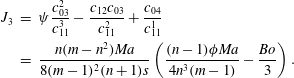 $$\begin{eqnarray}\displaystyle J_{3} & = & \displaystyle \unicode[STIX]{x1D713}\frac{c_{03}^{2}}{c_{11}^{3}}-\frac{c_{12}c_{03}}{c_{11}^{2}}+\frac{c_{04}}{c_{11}^{1}}\nonumber\\ \displaystyle & = & \displaystyle \frac{n(m-n^{2})Ma}{8(m-1)^{2}(n+1)s}\left(\frac{(n-1)\unicode[STIX]{x1D719}Ma}{4n^{3}(m-1)}-\frac{Bo}{3}\right).\end{eqnarray}$$
The leading term of
 $\text{Im}(\unicode[STIX]{x1D6FE})$
is
 $J_{3}\unicode[STIX]{x1D6FC}^{3}$
, and hence the leading phase velocity is
 $c=-\text{Im}(\unicode[STIX]{x1D6FE})/\unicode[STIX]{x1D6FC}=-J_{3}\unicode[STIX]{x1D6FC}^{2}$
. Thus, in contrast to the other branch, all the modes cannot be eliminated at once by applying an appropriate Galilean transformation.
The growth rate (4.3) is a continuous function of
 $\unicode[STIX]{x1D6FC}$
which is identified as the robust branch of the growth rate since it is non-zero even at
 $Ma=0$
. The other continuous branch of the growth rate, equation (4.5), that vanishes as
 $Ma\rightarrow 0$
, is the surfactant branch.
We note that there is another way to obtain the consecutive terms of the power series for the increment
 $\unicode[STIX]{x1D6FE}$
– by shuttling between the thickness and surfactant equations (3.27) and (3.28), with increasing powers in
 $\unicode[STIX]{x1D6FC}$
, to find the consecutive terms of the power series for the quantities
 $G/h$
and
 $\unicode[STIX]{x1D6FE}$
in turn. (This is equivalent to the method of undetermined coefficients.) It works slightly differently for the two modes, as follows:
For the surfactant mode, start with the thickness equation (3.27) at order
 $\unicode[STIX]{x1D6FC}^{1}$
to find
 $G/h$
to its leading order
 $\unicode[STIX]{x1D6FC}^{-1}$
. Use this in the surfactant equation taken at order
 $\unicode[STIX]{x1D6FC}^{1}$
to find
 $S_{2}$
. Apply the latter in the thickness equation at order
 $\unicode[STIX]{x1D6FC}^{2}$
to find the
 $\unicode[STIX]{x1D6FC}^{0}$
correction to the
 $G/h$
. Return with the latter to the surfactant equation taken at order
 $\unicode[STIX]{x1D6FC}^{2}$
to find
 $J_{3}$
.
For the robust mode, start with the thickness equation (3.27) at order
 $\unicode[STIX]{x1D6FC}^{1}$
and find
 $I_{1}$
. Use it in the surfactant equation at order
 $\unicode[STIX]{x1D6FC}^{1}$
to find
 $G/h$
to its leading order
 $\unicode[STIX]{x1D6FC}^{0}$
. Then the thickness equation at order
 $\unicode[STIX]{x1D6FC}^{2}$
yields
 $R_{2}$
. Next, the surfactant equation taken at order
 $\unicode[STIX]{x1D6FC}^{2}$
yields the
 $\unicode[STIX]{x1D6FC}^{1}$
correction to
 $G/h$
. The resulting expressions for the eigenfunctions
 $G/h$
are as follows. For the robust branch,
 $$\begin{eqnarray}\frac{G}{h}=-{\displaystyle \frac{\unicode[STIX]{x1D711}}{2n^{2}(m-1)}}+\text{i}\unicode[STIX]{x1D6FC}\frac{\unicode[STIX]{x1D713}}{4(m-1)^{2}n(n+1)s}\left(\frac{Bo}{3}-\unicode[STIX]{x1D719}\frac{(n-1)Ma}{4(m-1)n^{3}}\right),\end{eqnarray}$$
and for the surfactant branch,
 $$\begin{eqnarray}\frac{G}{h}=\text{i}{\displaystyle \frac{4(n+1)(m-1)s}{(n^{2}-m)Ma}}\unicode[STIX]{x1D6FC}^{-1}+\left({\displaystyle \frac{\unicode[STIX]{x1D713}(n-1)}{2n^{2}(n^{2}-m)(m-1)}}-{\displaystyle \frac{2Bon(n+m)}{3Ma(n^{2}-m)}}\right).\end{eqnarray}$$
Note that for
 $m=n^{2}$
(3.20) and (3.21) imply that for the surfactant branch
 $h=0$
and
 $G$
is arbitrary, and
 $\unicode[STIX]{x1D6FE}_{R}$
is consistent with (4.5). The latter two equations will be used in § 4.3.
For the case
 $s=0$
and
 $Bo=0$
, finding the leading-order growth rates requires the inclusion of capillary, fourth-derivative terms, which are found in the weakly nonlinear equations (3.22) and (3.23), and in the linear equations (3.27) and (3.28). The leading-order balance of the capillary and the Marangoni terms (the last two terms in (3.22)) yields in terms of the normal-mode amplitudes
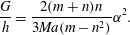 $$\begin{eqnarray}\frac{G}{h}=\frac{2(m+n)n}{3Ma(m-n^{2})}\unicode[STIX]{x1D6FC}^{2}.\end{eqnarray}$$
The leading-order balance in the surfactant transport equation involves three terms: the time derivative term; the capillary term; and the Marangoni term. Substituting in there
 $h$
in terms of
 $G$
from the preceding equation yields the growth rate of the robust mode:
 $$\begin{eqnarray}\unicode[STIX]{x1D6FE}_{R}=-\frac{n^{3}}{12(m+n^{3})}\unicode[STIX]{x1D6FC}^{4}.\end{eqnarray}$$
For the surfactant mode the capillary effects are negligible. So, the leading-order balance in the surfactant transport equation involves just the two terms with
 $G$
, and immediately yields the growth rate:
 $$\begin{eqnarray}\unicode[STIX]{x1D6FE}_{R}=-\frac{n(m+n^{3})Ma}{\unicode[STIX]{x1D713}}\unicode[STIX]{x1D6FC}^{2}.\end{eqnarray}$$
Substituting this into the kinematic condition yields
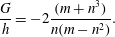 $$\begin{eqnarray}\frac{G}{h}=-2\frac{(m+n^{3})}{n(m-n^{2})}.\end{eqnarray}$$
These results are in agreement with FH.
Finally, for the case
 $s=0$
and
 $Bo\neq 0$
there is no universal expansion of the increment in powers of
 $\unicode[STIX]{x1D6FC}$
. However, it is easy to see that both modes are stable if
 $Bo>0$
but there is instability if
 $Bo<0$
. Indeed, if
 $Bo<0$
then
 $c_{0}=(1/12)n^{4}\unicode[STIX]{x1D6FC}^{4}MaBo<0$
(see (3.33)). Therefore in (3.34), the discriminant
 $c_{1}^{2}-4\unicode[STIX]{x1D713}c_{0}>c_{1}^{2}$
(note that for this case (3.32) yields
 $c_{1}=n\unicode[STIX]{x1D6FC}^{2}((m+n^{3})Ma+n(m+n)Bo/3)$
), and (3.31) yields one positive growth rate value, so we have an instability. This is essentially the Rayleigh–Taylor instability of a stagnant two-layer arrangement modified by the surfactant. On the other hand, if
 $Bo>0$
, then
 $c_{0}>0$
and
 $c_{1}>0$
, but the discriminant can be either positive or negative. If it is negative, then the square roots in the solution (3.34) are purely imaginary and therefore both values of
 $\unicode[STIX]{x1D6FE}_{R}$
are negative. If the discriminant is positive, then
 $|\sqrt{c_{1}^{2}-4\unicode[STIX]{x1D713}c_{0}}|<c_{1}$
, so that both values of
 $\unicode[STIX]{x1D6FE}$
given by (3.34) are negative again. It is clear that in all these cases
 $\unicode[STIX]{x1D6FE}\propto \unicode[STIX]{x1D6FC}^{2}$
. After the increment
 $\unicode[STIX]{x1D6FE}$
is determined from (3.34) (where the two possible values correspond to the two different modes), the eigenfunction
 $G/h$
is found from the kinematic condition (3.27) as
 $$\begin{eqnarray}\frac{G}{h}=\frac{2}{(m-n^{2})Ma}\left(\frac{\unicode[STIX]{x1D713}}{n^{2}}\unicode[STIX]{x1D6FC}^{-2}\unicode[STIX]{x1D6FE}+\frac{(m+n)nBo}{3}\right).\end{eqnarray}$$
We note that a growth rate ‘superposition principle’,
 $\unicode[STIX]{x1D6FE}_{R}(Ma,Bo)=\unicode[STIX]{x1D6FE}_{R}(Ma,0)+\unicode[STIX]{x1D6FE}_{R}(0,Bo)$
, holds for the robust branch at the leading order of (4.3). (The purely Marangoni growth rate
 $\unicode[STIX]{x1D6FE}_{R}(Ma,0)$
is the one found in FH, and the other, purely Bond, term gives the well-known growth rate of the (surfactantless) Rayleigh–Taylor instability.) In contrast, the leading-order growth rate of the surfactant branch, equation (4.5), is independent of the Bond number; the latter appears at higher orders, and is always multiplied by some positive power of the Marangoni number (see appendix A of Frenkel & Halpern (Reference Frenkel and Halpern2016)).
4.2 Instability thresholds in the three (
 $n,m$
)-sectors

From the long-wave approximation of FH, for
 $Bo=0$
, three sectors were identified in the
 $n\geqslant 1$
part of the
 $(n,m)$
-plane as regards the stability of the flow. The same three sectors turn out to be relevant even when
 $Bo\neq 0$
(as in our present case): the
 $Q$
sector (
 $1<n^{2}<m$
); the
 $R$
sector (
 $1<m<n^{2}$
); and the
 $S$
sector (
 $1<n<\infty$
and
 $0<m<1$
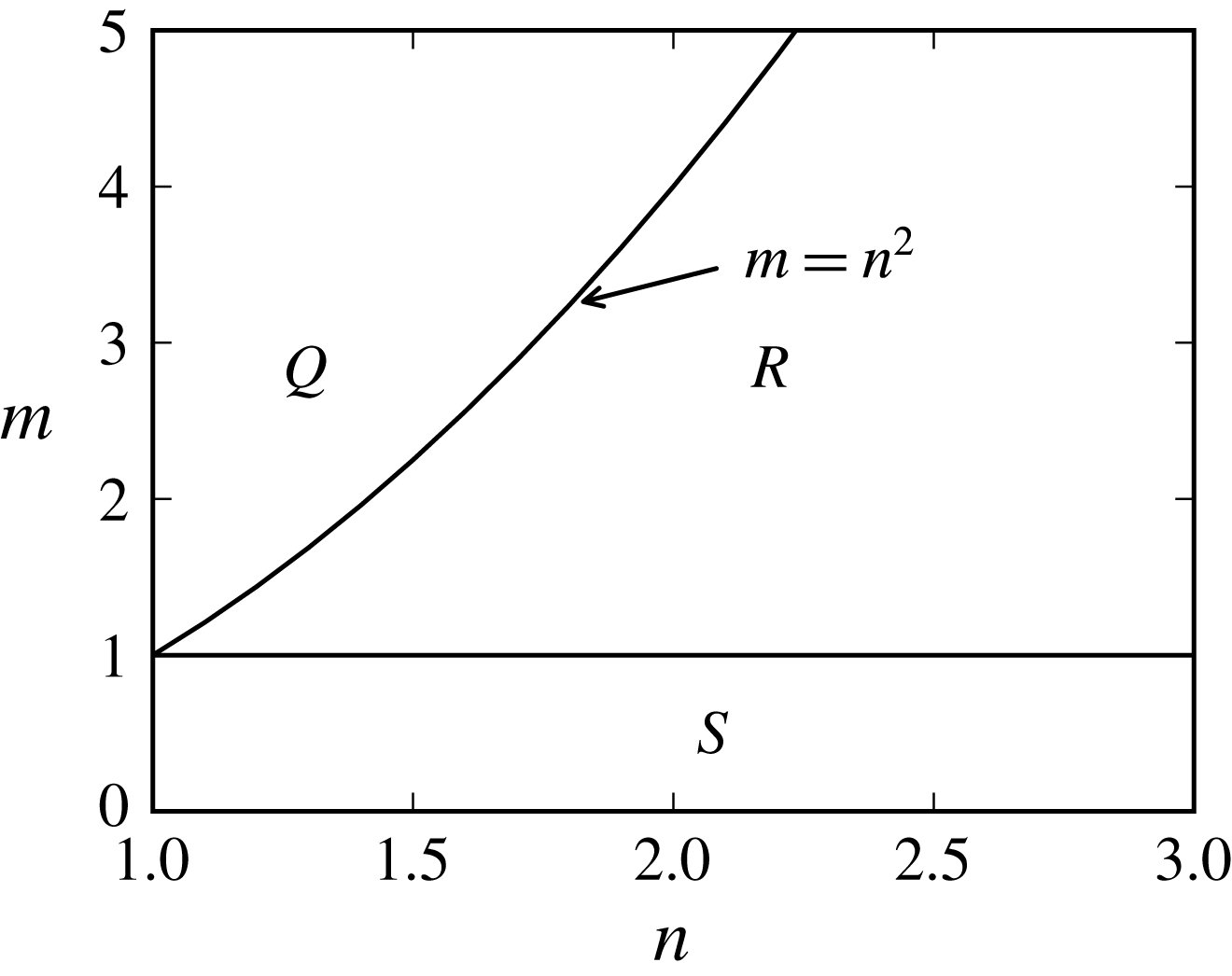
). (The boundaries between the sectors
 $m=n^{2}$
and
 $m=1$
correspond to the numerator and denominator respectively of the coefficient of the Marangoni number in (4.3). Therefore it is clear why they appear for the inertialess case of FH, with zero gravity and non-zero Marangoni number. We note that the same curves,
 $m=n^{2}$
and
 $m=1$
appear as neutral stability curves in the corrected figure 2 of Yiantsios & Higgins (Reference Yiantsios and Higgins1988) (see the correction Yiantsios & Higgins Reference Yiantsios and Higgins1989) for the case with neither surfactant nor gravity effects, where the instability hinges on inertia – despite the fact that Poiseuille flow, and not Couette flow, was the focus of attention in Yiantsios & Higgins (Reference Yiantsios and Higgins1988). Part of the reason for this is that the leading-order disturbance flow of the robust mode (obtained in § 5.4; see (A 5)) is a propagating wave which does not depend on the factors responsible for the growth or decay of the disturbances – such as inertia, gravity or surfactant effects. (Also, it does not depend on the details of the base velocity profile other than its interfacial slope.) Therefore, this leading-order disturbance flow, which contains the expressions
 $m-n^{2}$
and
 $m-1$
, is essentially the same (up to a scaling factor) for the Yih instability, the surfactant instability, or the Rayleigh–Taylor instability of the basic flow, whether Couette or Poiseuille one. Note, however, that for the inertial instability of the Couette flow in Yih (Reference Yih1967), despite the fact that the leading-order disturbance flow is still the same, the curve
 $m=n^{2}$
is not a curve of neutral stability. This is related to the following difference between the Yih instability and the inertialess instability. For the latter, the momentum equations for the correction of the disturbances are homogeneous, not depending on the base flow. Thus, they are the same for the Poiseuille flow
 $\bar{u}_{j}=(sz+qz^{2})/m_{j}$
, with
 $q(m-n^{2})=s(n+m)$
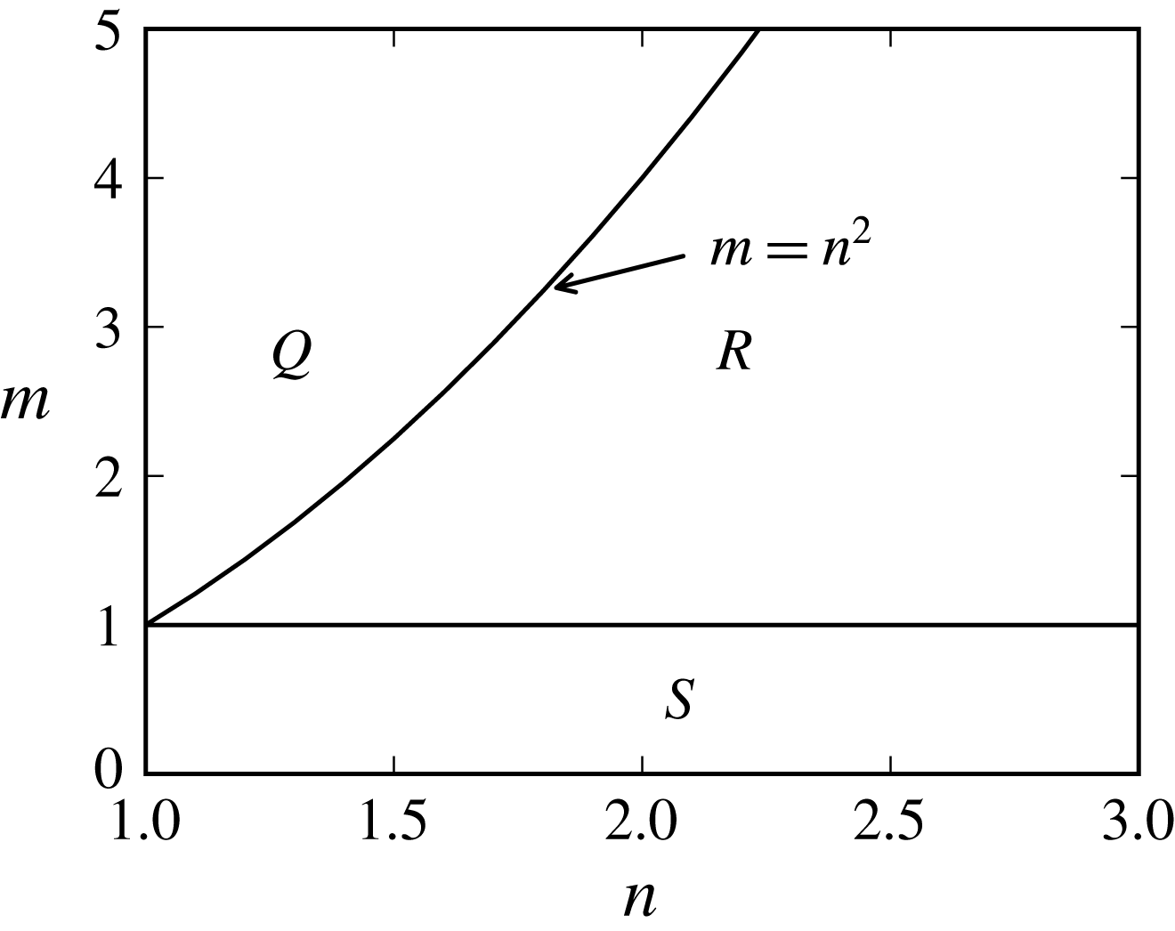
, as for the Couette flow, equations (2.13)–(2.14). In contrast, for the cases with non-zero inertia, the momentum equations for the disturbances at the correction order are non-homogeneous with their sources depending on the base flow and the leading-order disturbance of the flow. This is why the linear inertial instability results for the Poiseuille flow of Yiantsios & Higgins (Reference Yiantsios and Higgins1988) differ from those for the Couette flow of Yih (Reference Yih1967) and of Charru & Hinch (Reference Charru and Hinch2000) while the inertialess surfactant instability results would be the same for the Poiseuille flow as our results for the Couette flow.) Figure 2 shows the three sectors and their borders. Stability properties of the robust and surfactant modes can change significantly as one moves from sector to sector.
The
 $(n,m)$
-plane (for
 $n\geqslant 1$
) consists of three sectors (
 $Q$
,
 $R$
and
 $S$
) which differ as regards the flow stability properties.
In both the
 $R$
sector and the
 $Q$
sector, according to (4.5), the surfactant branch is stable for all
 $Bo$
. From (4.3) we can infer that the robust branch, is unstable if
 $Bo<Bo_{cL}$
, where the threshold value is
 $$\begin{eqnarray}Bo_{cL}=-\frac{3\unicode[STIX]{x1D711}(m-n^{2})}{4n^{3}(m-1)(n+m)}Ma.\end{eqnarray}$$
This condition holds for all three sectors, as does also the fact that gravity is stabilizing for
 $Bo>0$
and destabilizing for
 $Bo<0$
. In the
 $R$
sector, the Marangoni effect is destabilizing and, from (4.14) with
 $m<n^{2}$
, we have
 $Bo_{cL}>0$
. Gravity renders the flow stable for
 $Bo>Bo_{cL}$
, but for positive
 $Bo$
below
 $Bo_{cL}$
, the flow is still unstable (and it is unstable for all negative Bond numbers). In the
 $Q$
sector, the Marangoni effect is stabilizing,
 $Bo_{cL}<0$
, and gravity renders the flow unstable only for the negative Bond numbers below
 $Bo_{cL}$
. In another interpretation of the same relation, we say that surfactants with a given Marangoni number can stabilize the Rayleigh–Taylor instability, provided that
 $Bo$
is above the threshold (4.14)
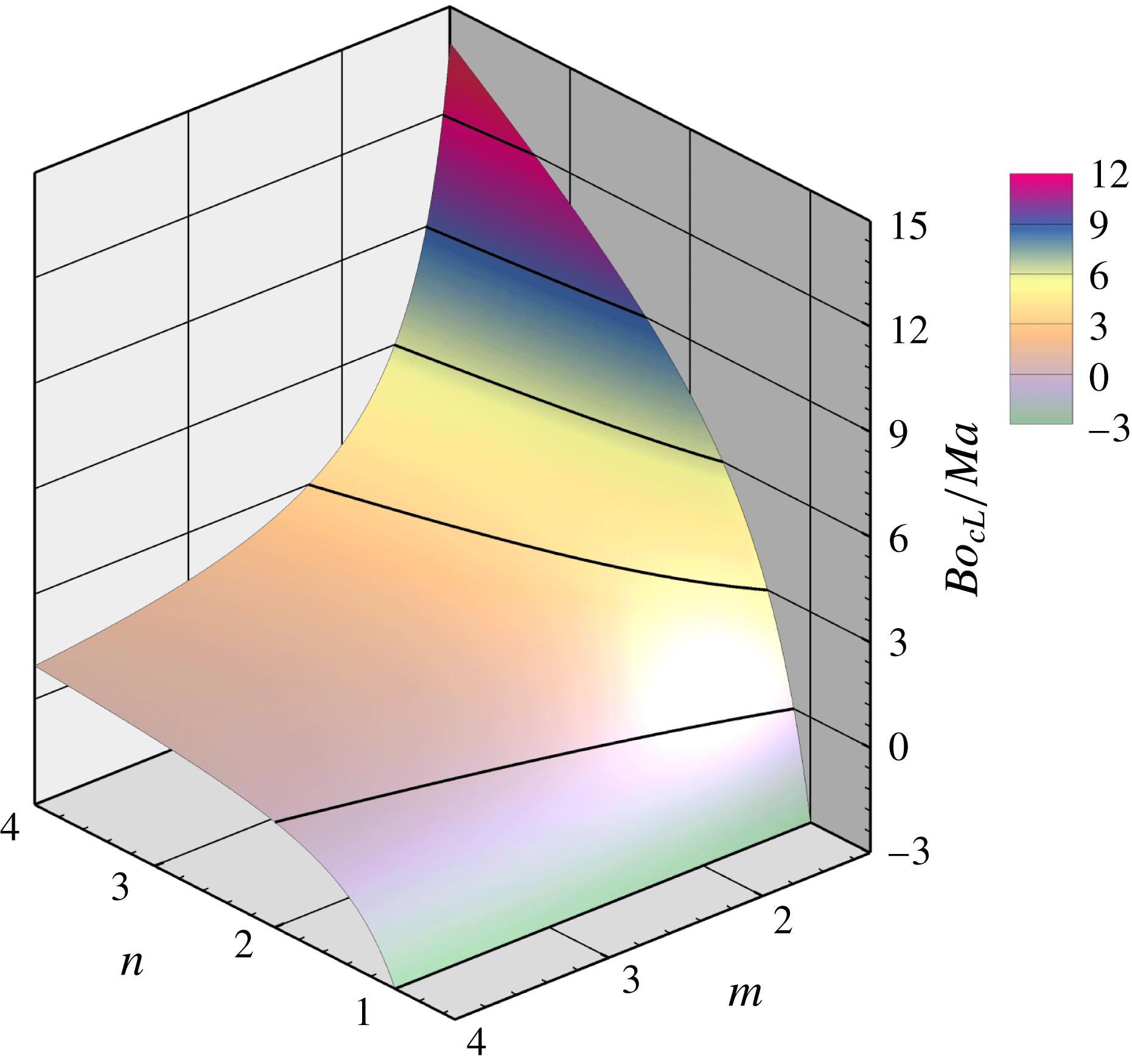
From (4.14) the ratio
 $Bo_{cL}/Ma$
is a function of
 $m$
and
 $n$
only, and its graph is a surface in the
 $(n,m,Bo_{cL}/Ma)$
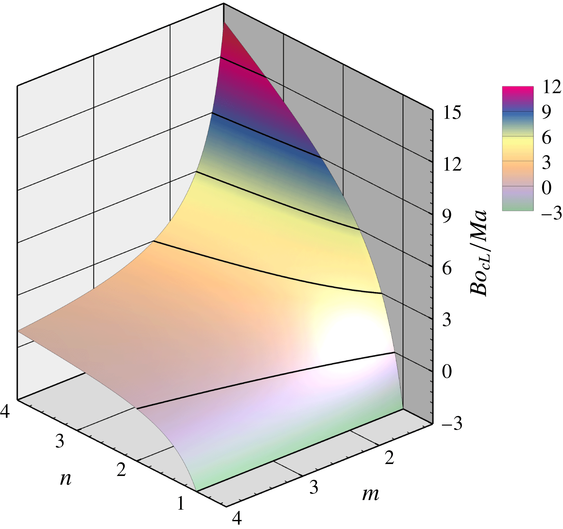
-space. Figure 3 represents the surface of the threshold ratio
 $Bo_{cL}/Ma$
for the
 $R$
and
 $Q$
sectors combined, that is for the region
 $n>1$
and
 $m>1$
. In particular, figure 3 reflects the fact (which is clear from (4.14), in view of the factor
 $m-1$
in the denominator) that
 $Bo_{cL}\uparrow \infty$
as
 $m\downarrow 1$
at a fixed
 $n$
(which implies the
 $R$
sector). This growth of
 $Bo_{cL}$
as
 $m\downarrow 1$
is especially pronounced for larger aspect ratios, as we see in the figure for the largest value included,
 $n=4$
; while for
 $n=1$
the critical ratio is constant,
 $Bo_{cL}/Ma=-3$
. (Because of the threshold ratio being infinite at
 $m=1$
, it is impossible to include in the figure all the values of
 $m$
down to
 $m=1$
; the cutoff in the figure 3 is at
 $m=1.3$
.) Also, from (4.14),
 $Bo_{cL}\downarrow 0$
as
 $m\rightarrow n^{2}$
(in both
 $R$
and
 $Q$
sectors). In figure 3, the corresponding zero-level horizontal cross-section is highlighted to appear different from the other horizontal cross-sections; it is, clearly, the curve
 $m=n^{2}$
in the coordinate
 $(n,m)$
-plane. In contrast to the
 $R$
sector, in the
 $Q$
sector the (negative)
 $Bo_{cL}$
, is bounded: equation (4.14) has a finite value at
 $n=1$
, and a finite limit as
 $m\uparrow \infty$
, since the expression
 $\unicode[STIX]{x1D711}$
(see (3.17)) is linear in
 $m$
.
The ratio
 $Bo_{cL}/Ma$
as a function of the aspect ratio and viscosity ratio for
 $n\geqslant 1$
and
 $m>1$
(in the
 $R$
and
 $Q$
sectors). Here
 $Ma=0.1$
and
 $s=1$
.
In the
 $S$
sector (
 $1<n<\infty$
and
 $0<m<1$
), the robust branch (4.3) is unstable when the Bond number is below the threshold value given by (4.14) (which is negative in this sector since the Marangoni action is stabilizing, in contrast to the
 $R$
sector) and stable otherwise. As to the surfactant branch in this sector, equation (4.5), which does not contain the Bond number, indicates instability. Thus the surfactant mode is unstable for any
 $Bo$
provided
 $\unicode[STIX]{x1D6FC}$
is sufficiently small. The conclusion that no amount of gravity can completely stabilize the flow may come across as somewhat counterintuitive.
We have omitted the stabilizing effects of capillary pressure since, as was explained before, we are concerned with the instability threshold and this is determined in the long-wave limit, in which these effects are negligible. More detailed linear stability results, including the asymptotic properties of the growth rate near the marginal wavenumber and also on the borders between the
 $Q$
,
 $R$
and
 $S$
sectors, are found (in a different way) in Schweiger (Reference Schweiger2013), and will be further investigated elsewhere.
4.3 Phase shifts and their limitations as regards criteria of stability
The surfactant-interface phase shift,
 $\unicode[STIX]{x1D703}_{G}:=\arg (G/h)$
,
 $-\unicode[STIX]{x03C0}<\unicode[STIX]{x1D703}_{G}\leqslant \unicode[STIX]{x03C0}$
, was considered in FH for a particular case, with no gravity,
 $m=1$
, and in the limit
 $n\rightarrow \infty$
, in order to make a plausibility argument about how the instability was possible – since there seemed to be in the literature the (erroneous) idea, based on systems with no base flow, that the surfactant is always stabilizing. The plausible ‘rule of surfactant phase interval’ seemed to be that stability corresponds to the phase shift being closer to the in-phase case, that is to being in the interval
 $(-\unicode[STIX]{x03C0}/2,\unicode[STIX]{x03C0}/2)$
(excluding its (corresponding to neutral stability) midpoint,
 $\unicode[STIX]{x1D703}_{G}=0$
). The analysis of the expressions (4.7) and (4.8) shows that in the absence of gravity this rule works also for the case (not considered in this regard in FH) with
 $m\neq 1$
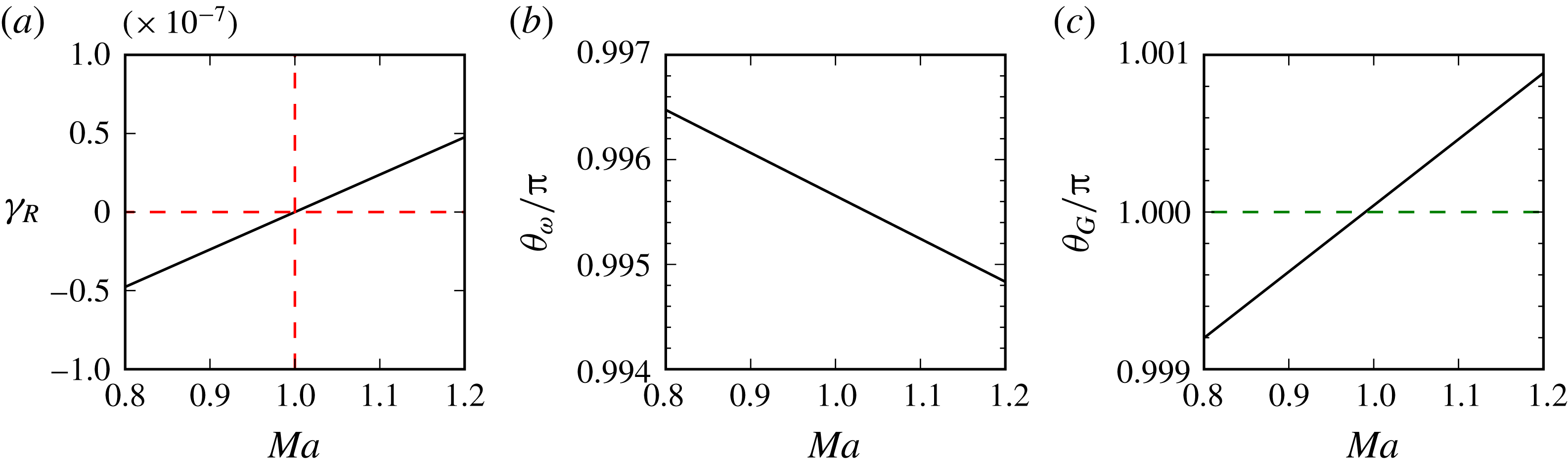
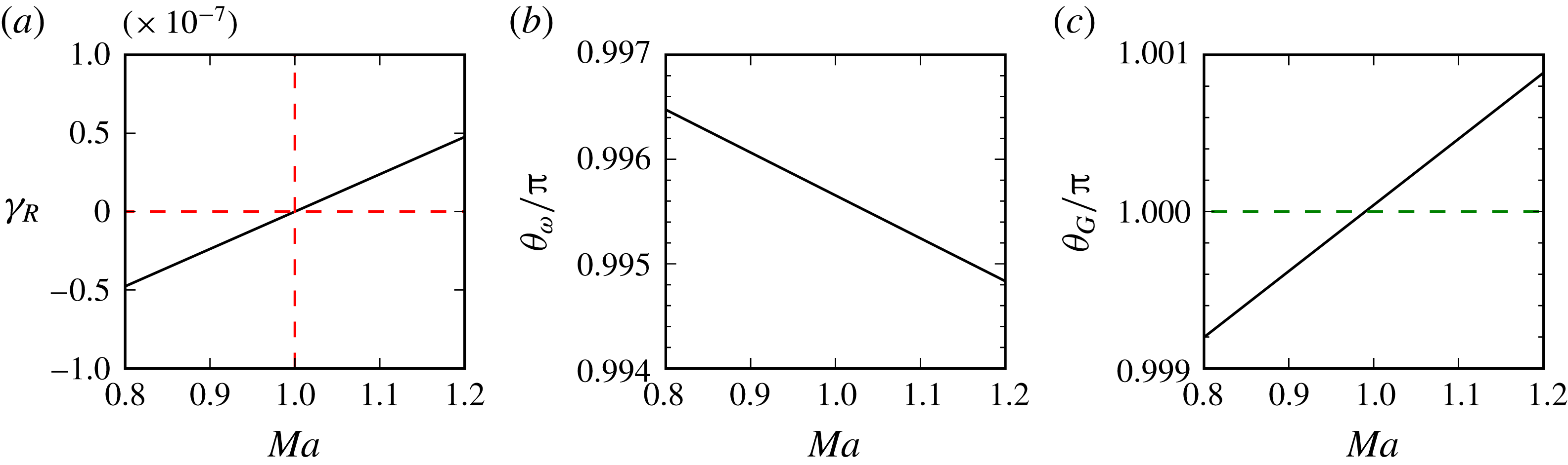
, and (bounded) channel flows. (See details in Frenkel & Halpern Reference Frenkel and Halpern2016.) However, in the presence of gravity this phase interval rule is fallible: figure 4, panel (c), shows that
 $\unicode[STIX]{x1D703}_{G}$
remains in the same interval, close to
 $\unicode[STIX]{x03C0}$
(or, equivalently, to
 $-\unicode[STIX]{x03C0}$
), as
 $Ma$
is increased through the threshold value
 $Ma=1$
, so that stability gives way to instability (as the
 $\unicode[STIX]{x1D6FE}_{R}$
shown in panel (a) of that figure testifies).
Dependencies on the Marangoni number for the robust mode in the
 $R$
sector, with
 $m=2$
,
 $n=100$
,
 $s=10$
and
 $\unicode[STIX]{x1D6FC}=10^{-4}$
: (a) growth rate; (b) phase difference between the disturbances of the interfacial vorticity and the interface; and (c) phase difference between surfactant and interface disturbances. Here
 $Bo=Bo_{cL}(Ma)=1$
, so that, as (a) shows, the growth rate
 $\unicode[STIX]{x1D6FE}_{r}$
crosses 0 at
 $Ma=1$
.
In Wei (Reference Wei2005) (referred to as W below), the attention was directed to the phase shift
 $\unicode[STIX]{x1D703}_{\unicode[STIX]{x1D714}}$
between the bottom-layer vorticity
 $\unicode[STIX]{x1D714}_{1}$
and the interface
 $h$
,
 $\unicode[STIX]{x1D703}_{\unicode[STIX]{x1D714}}:=\arg (\unicode[STIX]{x1D714}_{1}/h)$
,
 $-\unicode[STIX]{x03C0}<\unicode[STIX]{x1D703}_{\unicode[STIX]{x1D714}}\leqslant \unicode[STIX]{x03C0}$
, to argue that the vorticity
 $\unicode[STIX]{x1D714}$
is key to the instability mechanism, the same as was shown to be the case in Charru & Hinch (Reference Charru and Hinch2000) for the same Couette flow, but with no surfactant, with the instability hinging on inertia. In contrast to W, we allow for non-zero Bond number values (with the same assumptions of
 $s\neq 0$
and negligible capillary pressure as in W). Considering this more general case enables one to uncover the limitations of the statements on correlation of stability/instability with certain two non-intersecting subintervals which sum up to the full range of
 $\unicode[STIX]{x1D703}_{\unicode[STIX]{x1D714}}$
. The
 $y$
-component of the interfacial vorticity in the lower layer, denoted by
 $\unicode[STIX]{x1D714}_{1}$
, is, to the leading order in
 $\unicode[STIX]{x1D6FC}$
,
 $$\begin{eqnarray}\unicode[STIX]{x1D714}_{1}=u_{1z}(z=0)=A_{1}\end{eqnarray}$$
from (3.2). (Note that the sign in (4.15) is opposite to that in W. This is due to the fact that our coordinate axes are related to those of W by a rotation about the
 $x$
-axis, so that our spanwise axis (our
 $y$
-axis) is directed opposite to that of W (his
 $z$
-axis). This is the root of the opposite signs difference between the two spanwise components of the vorticity vector.) To find the phase
 $\unicode[STIX]{x1D703}_{\unicode[STIX]{x1D714}}$
of
 $\unicode[STIX]{x1D714}_{1}/h$
, we substitute the normal-modes expressions for
 $\unicode[STIX]{x1D702}$
and
 $\unicode[STIX]{x1D6E4}$
into the linear form of (3.15) to obtain
 $A_{1}$
in terms of
 $h$
and
 $G$
, and then substitute
 $G$
in terms of
 $h$
from (4.7) for the robust branch or (4.8) for the surfactant branch to find, to the two leading orders in
 $\text{i}\unicode[STIX]{x1D6FC}$
,
 $$\begin{eqnarray}\frac{\unicode[STIX]{x1D714}_{1}}{h}=-4\frac{(n^{3}+m)(m-1)s}{\unicode[STIX]{x1D713}}+\text{i}\frac{\unicode[STIX]{x1D6FC}}{\unicode[STIX]{x1D713}}\left(2n^{2}(n+1)mBo+\frac{\unicode[STIX]{x1D711}(n^{3}+3nm+4m)Ma}{2n(m-1)}\right)\end{eqnarray}$$
for the robust branch, and
 $$\begin{eqnarray}\frac{\unicode[STIX]{x1D714}_{1}}{h}={\displaystyle \frac{4(m-1)s}{n^{2}-m}}+\text{i}\unicode[STIX]{x1D6FC}\left({\displaystyle \frac{2n^{2}Bo}{3(n^{2}-m)}}-{\displaystyle \frac{(n^{3}+3nm+4m)(n-1)Ma}{2n(n^{2}-m)(m-1)}}\right)\end{eqnarray}$$
for the surfactant branch. (See details in Frenkel & Halpern Reference Frenkel and Halpern2016.) The ‘rule of the vorticity phase intervals’ that W suggests is that the interval
 $(-\unicode[STIX]{x03C0},0)$
of
 $\unicode[STIX]{x1D703}_{\unicode[STIX]{x1D714}}$
corresponds to stability and the interval
 $(0,\unicode[STIX]{x03C0})$
to instability. Our asymptotic analysis and numerical results show that even for large
 $n$
, this may not hold in the presence of gravity. (See details in Frenkel & Halpern (Reference Frenkel and Halpern2016), where it is also explained why the argument of W holds only if the Bond number and the vorticity of the top layer are sufficiently small (as determined by other parameters).) For example, panel (b) of the robust branch figure 4 shows that as the Marangoni number increases through its critical value, so that the instability growth rate increases from small negative values through 0 to small positive values as the instability sets in, the phase difference
 $\unicode[STIX]{x1D703}_{\unicode[STIX]{x1D714}}$
remains slightly below
 $\unicode[STIX]{x03C0}$
, that is inside the interval corresponding to stability according to the rule of the vorticity phase intervals. A similar figure for the surfactant branch (not shown here because of space limitations, but included in Frenkel & Halpern (Reference Frenkel and Halpern2016) as figure 4) also demonstrates the violation of the rule of the vorticity phase intervals.
In general, it is clear that, dynamically, only the surfactant is responsible for instability in the absence of gravity. The non-zero vorticity component is just one of the kinematic fields that are present even in the absence of surfactants. It is interesting to consider, instead of vorticity, the upward component of the disturbance velocity,
 $w_{1}$
, in the bottom layer. From the linear kinematic equation (3.29) it follows that
 $\unicode[STIX]{x1D6FE}_{R}=\text{Re}(w_{1}(0)/h)$
(and the wave velocity
 $c=-\unicode[STIX]{x1D6FC}^{-1}\text{Im}(w/h)$
). Hence, one obtains the universal ‘rule of the velocity phase intervals’ for stability/instability: we have instability when
 $\unicode[STIX]{x1D703}_{w}$
, the phase shift of the upward velocity
 $w_{1}(0)$
relative to the interface is in the interval
 $(-\unicode[STIX]{x03C0}/2,\unicode[STIX]{x03C0}/2)$
, and stability corresponds to the interior of the rest of the interval
 $(-\unicode[STIX]{x03C0},\unicode[STIX]{x03C0})$
, that is the open region
 $(-\unicode[STIX]{x03C0},-\unicode[STIX]{x03C0}/2)\cup (\unicode[STIX]{x03C0}/2,\unicode[STIX]{x03C0})$
. This rule holds even in the presence of gravity. However, to use it as a meaningful tool for deciding stability, one needs to find the velocities of the normal modes (without first finding the increments). This is done in the next section, where, however, the real part of
 $w_{1}(0)$
is used rather than its phase, and the instability mechanism is formulated in terms of the horizontal velocity constituents which have a quarter-circle phase shift relative to the interface wave.
5 Instability mechanisms: Marangoni stresses and out-of-phase velocities
In this section, we endeavour to elucidate the mechanism of instability for the two branches of normal modes, somewhat in the spirit of Charru & Hinch (Reference Charru and Hinch2000) (CH for short). Like them, we will sometimes use dimensional quantities. For simplicity, we omit the stars in their notations for the latter, and also omit tildes denoting disturbances; the context indications are sufficient for avoiding confusion. Like in CH, we first consider the case with large aspect ratio
 $n$
and no gravity; these restrictions will be relaxed in the last subsection of this section. (However, unlike CH, interfacial surfactant is present, and may cause instability despite the absence of inertia. In contrast, inertia is necessary for Yih’s instability treated in CH.) Similar to CH, all parameters other than
 $n$
are tentatively assumed to be of order one.
5.1 Robust branch in the limit of large aspect ratio
Considering a small-amplitude, normal-mode disturbance of the interface,
 $\unicode[STIX]{x1D702}=h\exp (\unicode[STIX]{x1D6F4}t)\cos \unicode[STIX]{x1D6FC}(x-ct)$
(where
 $\unicode[STIX]{x1D6F4}:=\text{Re}(\unicode[STIX]{x1D6FE})$
is by definition the growth rate, the real part of the increment, and
 $c:=-\unicode[STIX]{x1D6FC}^{-1}\text{Im}(\unicode[STIX]{x1D6FE})$
is the wave velocity), and first neglecting the surfactant disturbance, we can repeat the considerations of CH to find the same leading-order disturbance flows. Namely, the disturbance flow in the thick layer is a pressure-gradient-driven one with the zero net flow rate, that is (omitting hats for the amplitudes)
 $$\begin{eqnarray}u_{2}=u_{0}\left(1-{\displaystyle \frac{z}{d_{2}}}\right)\left(1-3{\displaystyle \frac{z}{d_{2}}}\right).\end{eqnarray}$$
Here
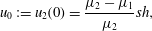 $$\begin{eqnarray}u_{0}:=u_{2}(0)=\frac{\unicode[STIX]{x1D707}_{2}-\unicode[STIX]{x1D707}_{1}}{\unicode[STIX]{x1D707}_{2}}sh,\end{eqnarray}$$
where
 $s$
is the (dimensional) base shear rate. (Note that the latter equation corresponds to the interfacial boundary condition for streamwise velocity components, equation (3.10) with
 $u_{2}=u_{2}(0)$
and
 $u_{1}=u_{1}(0)$
, in which
 $u_{1}(0)$
is neglected since it is much smaller than
 $u_{2}(0)$
.) Clearly, the pressure gradient is
 $6\unicode[STIX]{x1D707}_{2}u_{0}/d_{2}^{2}$
. Its interfacial shear stress drives a Couette flow in the thin layer,
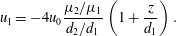 $$\begin{eqnarray}u_{1}=-4u_{0}\frac{\unicode[STIX]{x1D707}_{2}/\unicode[STIX]{x1D707}_{1}}{d_{2}/d_{1}}\left(1+\frac{z}{d_{1}}\right).\end{eqnarray}$$
(The two tangential stresses, of (5.1) and (5.3), are equal as they should be since for this branch the surfactant Marangoni stress is negligible at the leading order.) The balance of mass in a control volume [
 $0\leqslant x\leqslant \unicode[STIX]{x1D706}/2$
,
 $z<0$
] over a short time
 $0<t<\unicode[STIX]{x1D6FF}t$
gives, exactly as in CH, the wave velocity
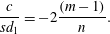 $$\begin{eqnarray}\frac{c}{sd_{1}}=-2\frac{(m-1)}{n}.\end{eqnarray}$$
(This result corresponds to the large
 $n$
limit of (4.2). Notably, the sign of
 $c$
is opposite to that of
 $m-1$
. We note also that while
 $u_{2}(0)\sim (1/n)^{0}$
, the transverse differentiation reduces the order:
 $Du_{2}(0)\sim (1/n)^{1}$
, which is then the order of the tangential stress; and
 $D^{2}u_{2}(0)\sim (1/n)^{2}$
, which is clearly the order of the pressure gradient
 $6\unicode[STIX]{x1D707}_{2}u_{0}/d_{2}^{2}$
.)
However, instead of originating from inertia, in our case the velocity correction to this flow, denoted
 $u_{1}^{M}$
, comes by the Marangoni action of the surfactant disturbance
 $\unicode[STIX]{x1D6E4}=|G|\exp (\unicode[STIX]{x1D6F4}t)$
 $\cos (\unicode[STIX]{x1D6FC}(x-ct)+\unicode[STIX]{x1D703}_{\unicode[STIX]{x1D6E4}})$
, where
 $\unicode[STIX]{x1D703}_{\unicode[STIX]{x1D6E4}}$
is a phase shift (undetermined for the moment), that is the argument of the complex amplitude of the surfactant eigenfunction,
 $G=|G|\exp \text{i}\unicode[STIX]{x1D703}_{\unicode[STIX]{x1D6E4}}$
. The Marangoni tangential stress should balance the viscous stress of the thin film, as the thick film contribution is much smaller in the interfacial condition (3.7); indeed, the interfacial (correction) velocities of the layers must be equal, and then the shear rate in the thick layer is
 $d_{1}/d_{2}$
times smaller than in the thin one. Thus, we find the linear velocity profile (satisfying also the no slip condition at the bottom plate):
 $$\begin{eqnarray}u_{1}^{M}=-\frac{\unicode[STIX]{x1D70E}_{0}}{\unicode[STIX]{x1D707}_{1}\unicode[STIX]{x1D6E4}_{0}}Ma\text{i}\unicode[STIX]{x1D6FC}G(z+d_{1}).\end{eqnarray}$$
(This corresponds to the large
 $n$
limit of the dimensionless equation (A 6). Similarly,
 $u_{2}^{M}$
would correspond to (A 8); however, like in CH, it is not needed in the argument. See an example of the profiles of these velocities in figure 5.) Note that the velocity phase here is
 $90^{\circ }$
less than that of the surfactant. The surfactant transport equation (2.9), at the leading order, yields
 $$\begin{eqnarray}\frac{\unicode[STIX]{x2202}\unicode[STIX]{x1D6E4}}{\unicode[STIX]{x2202}t}+\unicode[STIX]{x1D6E4}_{0}\frac{\unicode[STIX]{x2202}}{\unicode[STIX]{x2202}x}(\overline{u}_{1}(\unicode[STIX]{x1D702}))=0,\end{eqnarray}$$
where
 $\unicode[STIX]{x1D6E4}_{0}$
is the (uniform) base surfactant concentration and
 $\overline{u}_{1}(\unicode[STIX]{x1D702})=s\unicode[STIX]{x1D702}$
is the base velocity of the thin layer (2.13). Hence, in terms of the amplitudes, we get, at the leading order,
 $$\begin{eqnarray}-\!\text{i}c\unicode[STIX]{x1D6FC}G+\unicode[STIX]{x1D6E4}_{0}s\text{i}\unicode[STIX]{x1D6FC}h=0,\end{eqnarray}$$
or
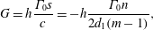 $$\begin{eqnarray}G=h\frac{\unicode[STIX]{x1D6E4}_{0}s}{c}=-h\frac{\unicode[STIX]{x1D6E4}_{0}n}{2d_{1}(m-1)},\end{eqnarray}$$
where the second equality follows from (5.4) which is the dimensional form of the large
 $n$
limit of the leading order in (4.7). (It follows that for
 $m>1$
the phase shift of the surfactant wave relative to the interface displacement wave is
 $\unicode[STIX]{x1D703}_{\unicode[STIX]{x1D6E4}}=\unicode[STIX]{x03C0}$
, i.e. they are in anti-phase, and for
 $m<1$
the phase shift is zero, so the surfactant disturbance is in phase with the interface displacement.) Substituting (5.8) into the velocity expression (5.5), we obtain the flow in terms of the interface displacement amplitude
 $h$
:
 $$\begin{eqnarray}u_{1}^{M}=h\frac{\unicode[STIX]{x1D70E}_{0}}{\unicode[STIX]{x1D707}_{1}}Ma\text{i}\unicode[STIX]{x1D6FC}\frac{n}{2(m-1)}\left(\frac{z}{d_{1}}+1\right).\end{eqnarray}$$
An illustration of the instability mechanism for
 $m=2$
,
 $n=6$
,
 $s=1$
,
 $Ma=0.01$
,
 $Bo=0$
and
 $\unicode[STIX]{x1D6FC}=10^{-4}$
. The velocity profiles at the end points of the control segment,
 $\unicode[STIX]{x1D706}/4\leqslant x\leqslant 3\unicode[STIX]{x1D706}/4$
where
 $\unicode[STIX]{x1D706}=2\unicode[STIX]{x03C0}/\unicode[STIX]{x1D6FC}$
is the wavelength, are shown for dimensionless out-of-phase disturbance velocities corresponding to (5.10) for the robust mode in (a). (b) Corresponds to the surfactant mode, which is stable for the same parameters.
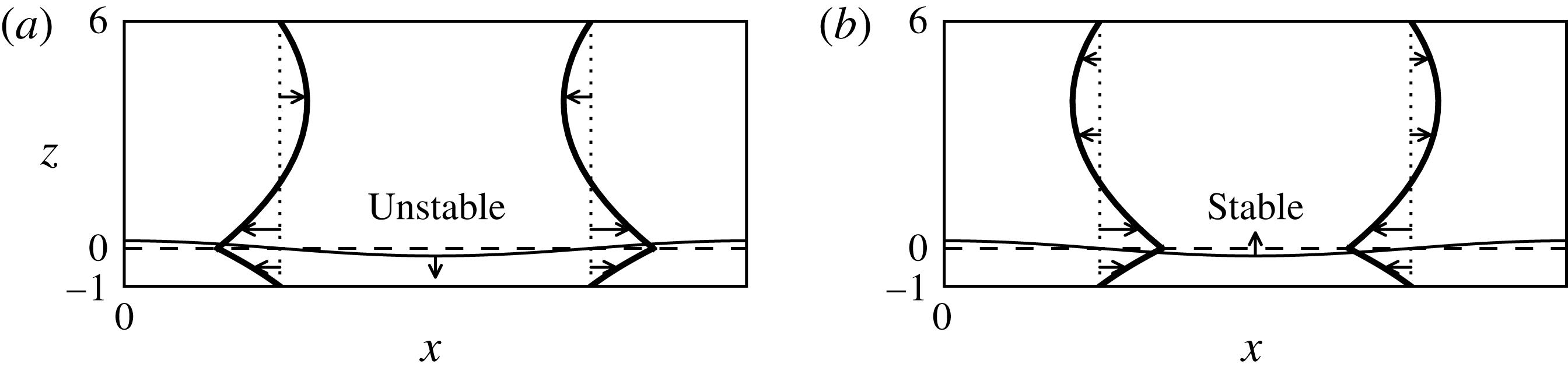
Since this velocity amplitude is purely imaginary, the velocity is out of phase with the interface, either by
 $90^{\circ }$
for
 $m>1$
, or
 $-90^{\circ }$
for
 $m<1$
. (We note that there is another correction velocity, of order
 $(1/n)^{2}$
, needed to satisfy the normal stress condition, the equality of pressures. However, its amplitude is real and hence it is either in phase or anti-phase with the interface, and not
 $\pm 90^{\circ }$
out-of-phase as in (5.9). Therefore, it leads to a small correction to the wave velocity, but is irrelevant to the growth rate.) The growth rate is found, as in CH, from the mass conservation law, by equating the change of volume of the thin layer over the interval
 $\unicode[STIX]{x1D706}/4\leqslant x\leqslant 3\unicode[STIX]{x1D706}/4$
(where
 $\unicode[STIX]{x1D706}:=2\unicode[STIX]{x03C0}/\unicode[STIX]{x1D6FC}$
is the wavelength), over a small time interval
 $\unicode[STIX]{x1D6FF}t$
, to the sum of inflow volumes through the two boundaries, at
 $x=\unicode[STIX]{x1D706}/4$
and
 $x=3\unicode[STIX]{x1D706}/4$
(at which point the flux magnitude attains its maximum, since the amplitude of the fluid flux is purely imaginary along with the velocity amplitude). Here, the inflow through the left boundary is given by the midlayer correction velocity, that is half the interfacial velocity at the boundary location, times the layer thickness
 $d_{1}$
, and that at the right boundary is similarly equal to minus the interfacial velocity at that boundary location times
 $d_{1}/2$
. The velocity at
 $x=\unicode[STIX]{x1D706}/4$
is
 $u_{1}^{M}(0)\exp \text{i}\unicode[STIX]{x1D6FC}\unicode[STIX]{x1D706}/4=\text{i}u_{1}^{M}(0)$
, where from (5.9),
 $$\begin{eqnarray}\text{i}u_{1}^{M}(0)=-h\frac{\unicode[STIX]{x1D70E}_{0}}{\unicode[STIX]{x1D707}_{1}}Ma\unicode[STIX]{x1D6FC}\frac{n}{2(m-1)}.\end{eqnarray}$$
The expression on the right-hand side here is similarly found to also give the negative of the velocity at the right boundary, so the two boundary inflows are exactly equal. (See an example in figure 5(a) which shows the flow corresponding to an unstable robust mode because
 $m>1$
. Panel (b) of this figure shows the flow corresponding to the surfactant mode which is stable for the same flow parameters as is discussed below in § 5.2.) As a result, the mass conservation equation is
 $$\begin{eqnarray}\text{i}u_{1}^{M}(0)d_{1}(\unicode[STIX]{x1D6FF}t)=\mathop{\int }_{\unicode[STIX]{x1D706}/4}^{3\unicode[STIX]{x1D706}/4}h(\text{e}^{\unicode[STIX]{x1D6F4}\unicode[STIX]{x1D6FF}t}-1)(\cos \unicode[STIX]{x1D6FC}x)\,\text{d}x=-\frac{2h\unicode[STIX]{x1D6F4}}{\unicode[STIX]{x1D6FC}}(\unicode[STIX]{x1D6FF}t).\end{eqnarray}$$
Substituting here for
 $\text{i}u_{1}^{M}(0)$
given by (5.10), we solve for the growth rate and obtain
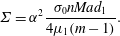 $$\begin{eqnarray}\unicode[STIX]{x1D6F4}=\unicode[STIX]{x1D6FC}^{2}\frac{\unicode[STIX]{x1D70E}_{0}nMad_{1}}{4\unicode[STIX]{x1D707}_{1}(m-1)}.\end{eqnarray}$$
(This result corresponds to the large
 $n$
limit of (4.3) with
 $Bo=0$
, and allows one to identify this mode as the robust one.) Clearly, this corresponds to instability for
 $m>1$
. Recall that for
 $m>1$
, the surfactant and the interface displacement are in anti-phase. For
 $m<1$
, we have in-phase propagation of the surfactant and interface displacement waves, hence the reversed velocities and consequently the stability of the normal mode. (A (different) link between the surfactant-interface phase shift and the stability of the normal mode was first noted in FH for a case with
 $m=1$
.)
A clearly equivalent way to this integral mass (of the fluid) conservation method of finding the growth rate is as follows. Use the divergenceless relation, with the horizontal velocity correction
 $u_{1}^{M}$
given by (5.9), to determine the vertical velocity correction
 $w_{1}^{M}(z=0)$
. Then the corresponding (real) correction to the increment is found from the linearized kinematic equation (3.29) to be
 $\unicode[STIX]{x1D6F4}=w_{1}^{M}(z=0)/h$
.
In summary, the growth/decay mechanism for the robust branch is described as follows. The leading-order flow is the same as in Yih (Reference Yih1967) and leads to the same, imaginary, increment. Then, the surfactant wave of the normal mode must propagate either in anti-phase for
 $m>1$
or in phase for
 $m<1$
with the interface. The Marangoni tangential stress exerted by the surfactant drives a (linear profile) correction flow whose velocity
 $u_{1}^{M}$
is
 $-90^{\circ }$
out of phase with the surfactant. Thus, this velocity is either
 $90^{\circ }$
for
 $m>1$
, or
 $-90^{\circ }$
for
 $m<1$
, out of phase with the interface. For
 $m>1$
, this leads to a net outflow for the half-period part of the thin layer with the thickness minimum at the middle point, that is instability for the normal mode, and for
 $m<1$
, the velocity is reversed, which yields stability. (Note that in difference with the Yih instability induced by inertia which was explained in Charru & Hinch (Reference Charru and Hinch2000) in terms of vorticity, the latter does not play any natural role in the mechanism of the surfactant-driven instability.)
5.2 Surfactant branch in the limit of large aspect ratio
In this subsection we consider the other normal mode, the surfactant mode. It turns out that here the surfactant effect appears at the leading order of disturbances. At the interface, the shear stress exerted on the thin layer by the thick layer (whose velocity is still given by (5.1)) and the Marangoni stress cancel each other to the leading order in
 $1/n$
. Therefore, the velocity is zero to this order, and hence the wave velocity to the order
 $\unicode[STIX]{x1D6FC}$
, in contrast to the robust mode, is zero. (There is a weak, pressure gradient related, flow in the thin layer, of order
 $(1/n)^{2}$
(see (A 1)); however, as was discussed regarding the robust mode, it is irrelevant to the growth rate, and actually gives a zero contribution to the increment.) The condition of such cancellation of the stresses is
 $$\begin{eqnarray}-\frac{4u_{0}\unicode[STIX]{x1D707}_{2}}{d_{2}}=\frac{\unicode[STIX]{x1D70E}_{0}}{\unicode[STIX]{x1D6E4}_{0}}Ma\text{i}\unicode[STIX]{x1D6FC}G.\end{eqnarray}$$
Using the expression for
 $u_{0}$
, equation (5.2), we find the following relation between
 $G$
and
 $h$
,
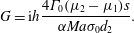 $$\begin{eqnarray}G=\text{i}h\frac{4\unicode[STIX]{x1D6E4}_{0}(\unicode[STIX]{x1D707}_{2}-\unicode[STIX]{x1D707}_{1})s}{\unicode[STIX]{x1D6FC}Ma\unicode[STIX]{x1D70E}_{0}d_{2}}.\end{eqnarray}$$
(Note that this is equivalent to the leading order in
 $\unicode[STIX]{x1D6FC}^{1}$
of
 $G/h$
found from the film-thickness equation (3.27), as in the first step in the ‘shuttling’ method discussed above. Also, note that this
 $G$
is purely imaginary (unlike being real for the robust mode), whereas the surfactant flux is always real at leading-order. Hence, the growth rate of the surfactant mode is found (immediately below) by using the surfactant conservation law in integral form.) One finds the growth rate of this branch by equating the change over a small time
 $\unicode[STIX]{x1D6FF}t$
of the total quantity of the surfactant over the interval
 $0\leqslant x\leqslant \unicode[STIX]{x1D706}/2$
, with the surfactant disturbance inflow through the interface boundaries, at
 $x=0$
and
 $x=\unicode[STIX]{x1D706}/2$
. The inflow rate is, at the leading order,
 $\unicode[STIX]{x1D6E4}_{0}\bar{u}_{1}(\unicode[STIX]{x1D702})=\unicode[STIX]{x1D6E4}_{0}sh\cos \unicode[STIX]{x1D6FC}x$
(note that this surfactant flux is in phase with the interface, and thus is positive (and maximum) at
 $x=0$
and negative at
 $x=\unicode[STIX]{x1D706}/2$
, corresponding to a positive net influx of the surfactant into the control part of the interface), which gives the sums of the inflows through the two boundaries to be
 $2\unicode[STIX]{x1D6E4}_{0}sh\unicode[STIX]{x1D6FF}t$
. The surfactant wave is
 $\unicode[STIX]{x1D6E4}=G_{I}\cos (\unicode[STIX]{x1D6FC}x+\unicode[STIX]{x03C0}/2)=-G_{I}\sin \unicode[STIX]{x1D6FC}x$
, where, in view of (5.14),
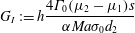 $$\begin{eqnarray}G_{I}:=h\frac{4\unicode[STIX]{x1D6E4}_{0}(\unicode[STIX]{x1D707}_{2}-\unicode[STIX]{x1D707}_{1})s}{\unicode[STIX]{x1D6FC}Ma\unicode[STIX]{x1D70E}_{0}d_{2}}\end{eqnarray}$$
is real. We see that the surfactant concentration reaches its minimum value at the middle point of the interval
 $0\leqslant x\leqslant \unicode[STIX]{x1D706}/2$
for
 $m>1$
, since then the phase shift of the surfactant (from the interface) is
 $90^{\circ }$
; but reaches its maximum value for
 $m<1$
since then the phase shift of the surfactant is
 $-90^{\circ }$
. Together with the aforementioned positive net influx of surfactant through the interval end points, this yields stability for
 $m>1$
and instability for
 $m<1$
. Quantitatively, the integral form of the mass conservation law for the surfactant implies
 $$\begin{eqnarray}2\unicode[STIX]{x1D6E4}_{0}sh(\unicode[STIX]{x1D6FF}t)=\mathop{\int }_{0}^{\unicode[STIX]{x1D706}/2}-G_{I}(\text{e}^{\unicode[STIX]{x1D6F4}\unicode[STIX]{x1D6FF}t}-1)(\sin \unicode[STIX]{x1D6FC}x)\,\text{d}x,=-\frac{2\unicode[STIX]{x1D6F4}(\unicode[STIX]{x1D6FF}t)G_{I}}{\unicode[STIX]{x1D6FC}}.\end{eqnarray}$$
(Note that this equation is equivalent to using the differential surfactant equation (3.28), which is the second step in the ‘shuttling’ method.) Substituting the expression (5.15) for
 $G_{I}$
, we arrive at the growth rate
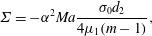 $$\begin{eqnarray}\unicode[STIX]{x1D6F4}=-\unicode[STIX]{x1D6FC}^{2}Ma\frac{\unicode[STIX]{x1D70E}_{0}d_{2}}{4\unicode[STIX]{x1D707}_{1}(m-1)},\end{eqnarray}$$
in agreement with the large
 $n$
limit of (4.5). Clearly, this formula shows stability for
 $m>1$
, which corresponds to the phase shift
 $\unicode[STIX]{x1D703}_{G}=$
 $\unicode[STIX]{x03C0}/2$
(see (5.14)), and instability for
 $m<1$
, corresponding to
 $\unicode[STIX]{x1D703}_{G}=$
 $-\unicode[STIX]{x03C0}/2$
.
This growth/decay mechanism is summarized as follows. The leading-order flow in the thick layer is the same as that for the robust branch, but vanishes in the thin layer because of the cancellation of the tangential stress of the thick layer by the Marangoni stress. This cancellation requires that the surfactant phase shift with respect to the interface is
 $90^{\circ }$
for
 $m>1$
and
 $-90^{\circ }$
for
 $m<1$
; whereas the surfactant flux (the product of the base concentration and the base velocity at the disturbed interface) is always in phase with the interface. Hence, the surfactant flux is out of phase with the surfactant wave,
 $90^{\circ }$
for
 $m>1$
and
 $-90^{\circ }$
for
 $m<1$
. Thus, considering the surfactant for
 $0\leqslant x\leqslant \unicode[STIX]{x1D706}/2$
, the net influx through the end points is always positive. For
 $m>1$
, the surfactant concentration is a minimum at the midpoint, and the positive influx implies stability. For
 $m<1$
, the surfactant concentration is a maximum at the midpoint, and the positive influx implies instability.
(If the assumed cancellation of the tangential stresses is relaxed, the two stresses in question are still of the same order, and this implies that
 $h\sim \text{i}\unicode[STIX]{x1D6FC}G$
. Since
 $u_{1}\sim h$
, we get
 $w_{1}(0)\sim \text{i}\unicode[STIX]{x1D6FC}h$
, and then (3.29) yields
 $\unicode[STIX]{x1D6FE}\sim \text{i}\unicode[STIX]{x1D6FC}$
. Hence, in the surfactant equation, the left-hand side term is
 $\unicode[STIX]{x1D6FE}G\sim \unicode[STIX]{x1D6FC}G$
, while no term on the right-hand side is of a lower order than
 $\text{i}\unicode[STIX]{x1D6FC}h\sim \unicode[STIX]{x1D6FC}^{2}G$
. Thus, the leading-order term
 $\unicode[STIX]{x1D6FE}G$
cannot be balanced. This contradiction can be resolved only by returning to the cancellation of the tangential stresses.)
As a consistency check, this growth rate, as well as the wave velocity for this branch, can be also recovered in the manner that was used for the other branch, by considering the volume balance of the bottom liquid film over the intervals of length
 $\unicode[STIX]{x03C0}/\unicode[STIX]{x1D6FC}$
, starting at
 $x=\unicode[STIX]{x03C0}/2\unicode[STIX]{x1D6FC}$
and
 $x=0$
, correspondingly. These calculations are found in Frenkel & Halpern (Reference Frenkel and Halpern2016).
5.3 Comparison of the two modes and intermediate asymptotics for large aspect ratio
In general, we may start the analysis for either mode with the disturbance flow in the thick layer. Remarkably, it is decoupled from the thin layer and is completely determined by the base flow and the condition of zero net flow in the thick layer. Returning to dimensionless quantities, this flow is
 $$\begin{eqnarray}u_{2}=\frac{(m-1)}{m}sh\left(1-\frac{z}{n}\right)\left(1-3\frac{z}{n}\right).\end{eqnarray}$$
It exerts a viscous tangential stress
 $\unicode[STIX]{x1D70F}_{2}=-4(m-1)sh/n$
on the thin layer at the interface. There is an additional tangential stress due to the Marangoni effect of the surfactant, which is
 $\unicode[STIX]{x1D70F}_{M}=-Ma\text{i}\unicode[STIX]{x1D6FC}G$
. The flow in the thin layer has a linear velocity profile driven by the sum of these two interfacial tangential stresses,
 $\unicode[STIX]{x1D70F}_{1}=\unicode[STIX]{x1D70F}_{2}+\unicode[STIX]{x1D70F}_{M}$
,
 $$\begin{eqnarray}u_{1}=-\frac{4(m-1)sh}{n}(z+1)-Ma\text{i}\unicode[STIX]{x1D6FC}G(z+1),\end{eqnarray}$$
where the first term is ultimately due to the base flow (via interfacial friction), and the second one to the surfactant. Using the continuity equation (3.3), we find the vertical velocity
 $$\begin{eqnarray}w_{1}(z)=\frac{2(m-1)s\text{i}\unicode[STIX]{x1D6FC}h}{n}(z+1)^{2}-\frac{1}{2}Ma\unicode[STIX]{x1D6FC}^{2}G(z+1)^{2}.\end{eqnarray}$$
We use the interfacial value of this velocity component to write the kinematic boundary condition (2.10) in the form
 $$\begin{eqnarray}\unicode[STIX]{x1D6FE}h-\frac{2s(m-1)}{n}\text{i}\unicode[STIX]{x1D6FC}h+\frac{Ma}{2}\unicode[STIX]{x1D6FC}^{2}G=0\end{eqnarray}$$
(cf. (3.27)). The second term here originates from the base flow and the third one is due to the surfactant. The surfactant transport equation (2.9) takes the form
 $$\begin{eqnarray}\unicode[STIX]{x1D6FE}G+\text{i}\unicode[STIX]{x1D6FC}sh+Ma\unicode[STIX]{x1D6FC}^{2}G=0\end{eqnarray}$$
(cf. (3.28)). Note that the term coming from the non-surfactant part of the disturbance velocity,
 $4(m-1)sh\text{i}\unicode[STIX]{x1D6FC}/n$
, has been neglected by comparison with the second term of (5.22).
There are three possibilities regarding the relative size of the Marangoni term (containing
 $MaG$
and corresponding to the Marangoni tangential stress at the interface) and the base flow term (containing
 $sh$
and corresponding to the interfacial tangential stress induced by the base flow) of the kinematic equation (5.21): (i) the Marangoni term is much smaller than the base flow term; (ii) both terms are of the same order; and (iii) the Marangoni term is much larger than the base flow term. We consider them in turn.
In the first case, when the Marangoni term is negligible, the kinematic equation gives
 $\unicode[STIX]{x1D6FE}=2\text{i}\unicode[STIX]{x1D6FC}s(m-1)/n$
to the leading order. Also, in this leading-order flow
 $G=-n/(2(m-1))h$
from the surfactant equation (cf. (5.8)). The surfactant-driven flow is a correction to this leading order, with the correction to increment
 $\unicode[STIX]{x1D6FE}_{c}$
satisfying the correction to the kinematic equation
 $$\begin{eqnarray}\unicode[STIX]{x1D6FE}_{c}h=-\frac{Ma}{2}\unicode[STIX]{x1D6FC}^{2}G=\frac{Man}{4(m-1)}\unicode[STIX]{x1D6FC}^{2}h.\end{eqnarray}$$
So the growth rate is
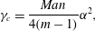 $$\begin{eqnarray}\unicode[STIX]{x1D6FE}_{c}=\frac{Man}{4(m-1)}\unicode[STIX]{x1D6FC}^{2},\end{eqnarray}$$
which is the dimensionless form of the result (5.12), the robust branch.
Assuming now the second case, the last two terms of the kinematic equation being of the same order
 $h/n\sim \unicode[STIX]{x1D6FC}G$
, it is clear that the Marangoni term in the transport equation is negligible. At a fixed
 $n$
, a solution can be found if the first term in the kinematic equation (5.21) is negligible. Then we have
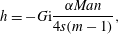 $$\begin{eqnarray}h=-G\text{i}\frac{\unicode[STIX]{x1D6FC}Man}{4s(m-1)},\end{eqnarray}$$
which agrees with the large
 $n$
limit of the leading order in (4.8). With this, the transport equation (5.22) yields
 $$\begin{eqnarray}\unicode[STIX]{x1D6FE}=-\frac{\unicode[STIX]{x1D6FC}^{2}Man}{4(m-1)},\end{eqnarray}$$
which is the dimensionless form of the previous result (5.17), the surfactant mode. Thus the two normal modes are characterized in terms of the relative strengths of the two tangential stresses at the interface.
Turning now to the last case, when the term with
 $Ma$
dominates the term with
 $s$
in the kinematic equation, we must have
 $\unicode[STIX]{x1D6FC}h/n\ll \unicode[STIX]{x1D6FC}^{2}G$
and hence
 $h\ll \unicode[STIX]{x1D6FC}nG\ll G$
(since
 $\unicode[STIX]{x1D6FC}n\ll 1$
), and the transport and kinematic equations simplify to
 $$\begin{eqnarray}\unicode[STIX]{x1D6FE}G=-\text{i}\unicode[STIX]{x1D6FC}sh\end{eqnarray}$$
and
 $$\begin{eqnarray}\unicode[STIX]{x1D6FE}h=-\unicode[STIX]{x1D6FC}^{2}MaG/2,\end{eqnarray}$$
respectively. From these two equations, we obtain
 $\unicode[STIX]{x1D6FE}^{2}=\text{i}\unicode[STIX]{x1D6FC}^{3}Mas/2$
, so
 $$\begin{eqnarray}\unicode[STIX]{x1D6FE}=\pm (1+\text{i})Ma^{1/2}s^{1/2}\unicode[STIX]{x1D6FC}^{3/2}/2.\end{eqnarray}$$
Thus, the growth rates for the two modes are
 $$\begin{eqnarray}\unicode[STIX]{x1D6F4}=\pm Ma^{1/2}s^{1/2}\unicode[STIX]{x1D6FC}^{3/2}/2,\end{eqnarray}$$
so one of the modes is stable and the other one unstable. Writing the fact that the second term in the kinematic equation is negligible in comparison with the third term,
 $h\ll \unicode[STIX]{x1D6FC}nG$
, and taking into account that, from the simplified transport equation with
 $\unicode[STIX]{x1D6FE}\sim \unicode[STIX]{x1D6FC}^{3/2}$
, we have
 $G\sim \unicode[STIX]{x1D6FC}^{-1/2}h$
, it follows that
 $1\ll \unicode[STIX]{x1D6FC}^{1/2}n$
. Together with
 $\unicode[STIX]{x1D6FC}n\ll 1$
, this means that the modes (5.30) exist in the interval
 $$\begin{eqnarray}\frac{1}{n^{2}}\ll \unicode[STIX]{x1D6FC}\ll \frac{1}{n},\end{eqnarray}$$
which is bounded away from zero. Thus, this case is generic, but the asymptotics (5.30) is merely intermediate since it does not persist in the limit
 $\unicode[STIX]{x1D6FC}\downarrow 0$
. One should note that the condition of validity for
 $\unicode[STIX]{x1D6FC}$
is more accurately given by
 $$\begin{eqnarray}\unicode[STIX]{x1D6FC}\ll \frac{1}{n}\ll \unicode[STIX]{x1D6FC}^{1/2}.\end{eqnarray}$$
5.4 Cases of the finite aspect ratio with possible gravity effects
Turning next to the less simple situation of the layer thicknesses being comparable, allowing for gravity effects, the flows in the two layers are fully coupled. Both governing equations, the kinematic equation (3.27) and the transport equation (3.28), have three different terms in their right-hand sides: one term due to the base shear (containing
 $sh$
), one due to the surfactant (containing
 $MaG$
), and one due to gravity (containing
 $Boh$
). The two modes found previously still have the following physical characterization, similar to the simpler case of large aspect ratio and no gravity: the robust mode has the gravity and surfactant effects absent at the leading order in
 $\text{i}\unicode[STIX]{x1D6FC}$
, so that only the first right-hand side term is retained in both governing equations. The simplified kinematic equation at once yields the leading-order increment (see (4.2))
 $$\begin{eqnarray}\unicode[STIX]{x1D6FE}=\frac{2\text{i}\unicode[STIX]{x1D6FC}(m-1)n^{2}(n+1)s}{\unicode[STIX]{x1D713}},\end{eqnarray}$$
(and thus the wave velocity
 $c=2(m-1)(n+1)n^{2}s/\unicode[STIX]{x1D713}$
). Therefore, the simplified surfactant transport equation determines
 $$\begin{eqnarray}G=-h\frac{\unicode[STIX]{x1D711}}{2n^{2}(m-1)}.\end{eqnarray}$$
(Note that this
 $G$
is real and hence the surfactant is either in phase (for
 $m<1$
) or in anti-phase (for
 $m>1$
) with the interface.) Thus, the leading order yields just the wave velocity found in Yih (Reference Yih1967) (and, for large
 $n$
, reproduces the previously obtained expression (5.4)). The growth rate due to surfactant and gravity effects appears in the correction to the leading-order disturbance flow. Substituting the leading order
 $G$
(5.34) into the kinematic equation (3.27) with the left-hand side
 $\unicode[STIX]{x1D6FE}_{c}h$
, where
 $\unicode[STIX]{x1D6FE}_{c}$
is the correction to the increment, and the first term on the right-hand side absent in the correction equation, we reproduce the growth rate (4.3) of the robust mode.
The surfactant mode hinges on the Marangoni effect, the leading-order flow being determined, just like in the previous case of large
 $n$
, by the dominant balance of only the base shear and surfactant terms in the kinematic equation. This reproduces the leading order of the result (4.8) for the relation between
 $G$
and
 $h$
, which we write now in the form
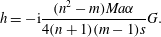 $$\begin{eqnarray}h=-\text{i}{\displaystyle \frac{(n^{2}-m)Ma\unicode[STIX]{x1D6FC}}{4(n+1)(m-1)s}}G.\end{eqnarray}$$
(Hence, the surfactant shift from the interface is
 $-90^{\circ }$
in the
 $S$
(
 $m<1$
) and
 $Q$
(
 $m>n^{2}$
) sectors and
 $90^{\circ }$
in the
 $R$
(
 $1<m<n^{2}$
) sector.) Substituting this into the surfactant transport equation (3.28), the gravity term is of a higher order in
 $\unicode[STIX]{x1D6FC}$
, and hence the growth rate is found to be independent of
 $Bo$
, reproducing equation (4.5).
One way to find the velocity profile
 $u_{1}(z)$
for the surfactant branch is to apply the same procedure as was used in § 5.2 for the case of large
 $n$
and no gravity. Namely, we use expression (3.2) for normal modes along with the linearized pressure gradient (3.14) and the interfacial vorticity (3.15) to obtain the velocity amplitude in terms of
 $G$
and
 $h$
, and then substitute
 $G$
in terms of
 $h$
from (4.8). The result is
 $$\begin{eqnarray}\displaystyle u_{1}(z) & = & \displaystyle -\frac{(m-1)s}{m-n^{2}}h(z+1)(3z+1)\nonumber\\ \displaystyle & & \displaystyle +\,\frac{\text{i}\unicode[STIX]{x1D6FC}h}{m-n^{2}}\left\{\frac{(n-1)Ma}{2(m-1)n}[3m(n+1)(z^{2}-1)+(4m+3mn+n^{3})(z+1)]\right.\nonumber\\ \displaystyle & & \displaystyle -\left.\frac{n^{2}Bo}{6}(z+1)(3z+1)\right\}.\end{eqnarray}$$
(All the other velocities, for both branches and both layers, can be found similarly, and are listed in appendix A.) As was noted in CH, any flow of this type, with a complex-valued horizontal velocity amplitude as in (5.36), can be considered as a superposition of two flows, one of which is in phase or anti-phase with the interface and the other is
 $\pm 90^{\circ }$
out of phase with the interface. The in-phase (or anti-phase) and out-of-phase flows correspond, respectively, to the real and purely imaginary addends in the amplitude of the horizontal velocity. The real part of this velocity component generates the imaginary part of the vertical velocity, whose interfacial value divided by
 $h$
equals the imaginary part of the increment, which determines the wave velocity; while the imaginary part generates the real part of the vertical velocity, whose interfacial value divided by
 $h$
is the growth rate. Thus, the stability/instability is due solely to the out-of-phase flow. (From the alternative point of view based on the integral form of the mass conservation law, this is so because the fluid flux wave is
 $\pm 90^{\circ }$
out of phase with the thickness wave.) Note that, in difference with the robust branch, whose in-phase flow is due to the base shear only, the in-phase flow of (5.36), a surfactant mode, has a contribution from the surfactant. This is due to the fact that, for the surfactant branch, to the leading order
 $\unicode[STIX]{x1D6FC}^{-1}$
, the surfactant amplitude
 $G$
is purely imaginary, i.e.
 $\pm 90^{\circ }$
out of phase with
 $h$
, and so expressing
 $G$
in terms of
 $h$
converts the surfactant terms in the pressure, vorticity, velocity and the kinematic equations into the form of the base shear terms there. The wave velocity, which corresponds to the real part of (5.36), vanishes since
 $\int _{-1}^{0}(z+1)(3z+1)\,\text{d}z=0$
. (For the same reason, there is no term proportional to
 $Bo$
in the growth rate (4.5) determined by the out-of-phase flow, by integrating the imaginary part of
 $u_{1}$
(5.36).) Also, this integral being zero is interpreted as the annihilation of the flux of the in-phase flow.
From these considerations, it transpires that the robust modes can be regarded as a modification of the (single) mode of Charru & Hinch (Reference Charru and Hinch2000), in which the leading-order flow is the same in-phase, non-dissipative Yih wave, but the next-order, out-of-phase, dissipative correction is determined, instead of inertia, by the Marangoni tangential stress and/or the pressure difference generated by the gravitational normal stress. Thus, the robust mode corresponds to the Marangoni tangential stress being of higher order than that of the tangential viscous stresses of the liquid layers (whose thicknesses are comparable) at their interface. The robust branch is also characterized by the leading-order surfactant concentration being either in phase or totally,
 $180^{\circ }$
out of phase with the interface, while for the surfactant branch the leading-order surfactant concentration is
 $\pm 90^{\circ }$
out of phase with the interface. The surfactant mode can be recovered, in this more physical way, by starting with the only other possible assumption about the Marangoni tangential stress: that the latter is of the same order as the viscous stresses of the liquid layers, and thus participates in the leading-order interfacial balance of the tangential stresses (and not only in the correction order of the tangential stress condition, as in the robust mode).
In more detail, in this alternative way of finding the complete normal modes
 $[u_{j}(z),w_{j}(z),p_{j},h,G]\text{e}^{\text{i}\unicode[STIX]{x1D6FC}x+\unicode[STIX]{x1D6FE}t}$
, the corresponding algebra-differential eigenvalue problem is given by the normal-form version of (3.1), (3.3), (3.5), (3.7), (3.10), (3.11), the kinematic equation
 $\unicode[STIX]{x1D6FE}h=w(0)$
(obtained by the linearization of (5.21) and the amplitude form of the linearized surfactant evolution equation (2.9) (with the diffusion term discarded):
 $$\begin{eqnarray}\unicode[STIX]{x1D6FE}G=-\text{i}\unicode[STIX]{x1D6FC}(sh+u_{1}(0)).\end{eqnarray}$$
There are also the zero conditions for the both velocity components at the plates. The solutions of the eigenvalue problems corresponding to the two branches of normal modes are obtained using the appropriate assumptions about the tangential stresses and the flow fluxes in the two layers (as was mentioned above).
We deal with the surfactant branch first. From the momentum equations, we know that the horizontal velocities are quadratic functions of
 $z$
that can be written, without loss of generality, in the form satisfying the no-slip wall conditions, as
 $$\begin{eqnarray}u_{1}=(z+1)[A_{1}(z-1)+A_{0}]\quad \text{and}\quad u_{2}=(z-n)[B_{1}(z+n)+B_{0}],\end{eqnarray}$$
(cf. (3.2). The same considerations hold for the robust branch, and below we will use for this velocity the same form with four undetermined coefficients.) Integrating the incompressibility equation yields the vertical velocities given by (A 19):
 $$\begin{eqnarray}w_{1}(z)=-\text{i}\unicode[STIX]{x1D6FC}\int _{-1}^{z}u_{1}(\unicode[STIX]{x1D709})\,\text{d}\unicode[STIX]{x1D709}\quad \text{and}\quad w_{2}(z)=-\text{i}\unicode[STIX]{x1D6FC}\int _{n}^{z}u_{2}(\unicode[STIX]{x1D709})\,\text{d}\unicode[STIX]{x1D709}.\end{eqnarray}$$
For the surfactant branch, as discussed above, the Marangoni stresses act already in the leading order, and in such a way that, to the leading order (but not necessarily for the correction, as will be seen later), the fluxes vanish through each layer separately. This is equivalent to requiring
 $w_{1}(0)=w_{2}(0)=0$
(which, from the kinematic condition, implies that the leading-order
 $\unicode[STIX]{x1D6FC}^{1}$
increment is zero). Integrating (5.39) with the upper limit
 $z=0$
yields the following two relations for the coefficients:
 $$\begin{eqnarray}-\!{\textstyle \frac{2}{3}}A_{1}+{\textstyle \frac{1}{2}}A_{0}=0\quad \text{and}\quad {\textstyle \frac{2}{3}}n^{3}B_{1}+{\textstyle \frac{1}{2}}n^{2}B_{0}=0.\end{eqnarray}$$
This allows eliminating two of the constants and thus writing each velocity with just one undetermined coefficient:
 $u_{1}=A(z+1)(3z+1)sh$
and
 $u_{2}=B(z-n)(3z-n)sh$
, (where the factor
 $sh$
has been introduced for future convenience). The pressures are equal since the gravity effects are of a higher order; this requires
 $mB=A$
. Hence, we eliminate
 $A$
from the interfacial condition for the horizontal velocities, at
 $z=0$
:
 $n^{2}Bsh-mBsh=sh(m-1)/m$
. This implies the solution
 $$\begin{eqnarray}B=\frac{(m-1)}{m(n^{2}-m)},\quad A=\frac{(m-1)}{(n^{2}-m)}.\end{eqnarray}$$
With this, we obtain exactly the leading-order velocities (A 1) and (A 3). Next, the tangential stress condition (3.7), written in the amplitude form, gives a relation between
 $h$
and
 $G$
,
 $4sh(n+1)(m-1)/(m-n^{2})=\text{i}\unicode[STIX]{x1D6FC}MaG$
(thus reproducing the leading-order of (4.8)), which we use in the following amplitude form of the linearized surfactant evolution equation (2.9) (with the diffusion term discarded):
 $$\begin{eqnarray}\unicode[STIX]{x1D6FE}G=-\text{i}\unicode[STIX]{x1D6FC}(sh+u_{1}(0)),\end{eqnarray}$$
where
 $u_{1}(0)=-sh(m-1)/(m-n^{2})$
. Substituting the latter into the surfactant equation (5.42), followed by expressing
 $h$
in terms
 $G$
from the tangential stress condition, yields, after cancelling out
 $G$
, exactly the explicit expression (4.5) for the leading-order increment
 $\unicode[STIX]{x1D6FE}$
(which is real and thus the leading-order non-zero growth rate for the surfactant mode).
The (purely imaginary, out of phase with
 $h$
) corrections to these leading-order disturbances of the horizontal velocities are written in the same quadratic form (5.38), but with the four coefficients having the superscript ‘
 $c$
’ and, for anticipated convenience, a factor
 $\text{i}\unicode[STIX]{x1D6FC}h$
. However, in contrast to the leading order, each correction flux is not required to be zero; instead, the kinematic condition in order
 $\unicode[STIX]{x1D6FC}^{2}$
requires
 $w_{1}^{c}(0)=\unicode[STIX]{x1D6FE}=w_{2}^{c}(0)$
where
 $\unicode[STIX]{x1D6FE}$
is the leading-order growth rate given by (4.5). This yields the following two relations for the coefficients:
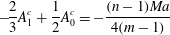 $$\begin{eqnarray}-\!\frac{2}{3}A_{1}^{c}+\frac{1}{2}A_{0}^{c}=-\frac{(n-1)Ma}{4(m-1)}\end{eqnarray}$$
and
 $$\begin{eqnarray}n^{3}B_{1}^{c}+\frac{1}{2}n^{2}B_{0}^{c}=-\frac{(n-1)Ma}{4(m-1)}.\end{eqnarray}$$
We use the latter equation to express
 $B_{0}^{c}$
in terms of
 $B_{1}^{c}$
and
 $Ma$
. From the normal stress condition, we obtain
 $A_{1}^{c}$
in terms of
 $B_{1}^{c}$
and
 $Bo$
. Then, using the continuity of the horizontal velocities at
 $z=0$
,
 $A_{0}^{c}$
is obtained in terms of
 $B_{1}^{c}$
,
 $Bo$
and
 $Ma$
. Substituting the latter expressions into (5.43) yields an equation for
 $B_{1}^{c}$
, whose solution is
 $$\begin{eqnarray}B_{1}^{c}=\frac{1}{2(m-n^{2})}\left(Ma\frac{3(n^{2}-1)}{(m-1)n}-Bo\right).\end{eqnarray}$$
Using this, all the other coefficients are written in terms of the system parameters, which reproduces the imaginary parts of the horizontal velocity eigenfunctions, equations (A 2) and (A 4) of appendix A. The tangential stress condition (3.7), in this order, leads to the relation
 $\text{i}\unicode[STIX]{x1D6FC}h(mB_{0}^{c}-A_{0}^{c})=\text{i}\unicode[STIX]{x1D6FC}MaG^{c}$
, from which we obtain the
 $G^{c}/h$
in terms of the parameters. It is exactly the second term of (4.8). Finally, the surfactant equation of the order
 $\unicode[STIX]{x1D6FC}^{2}$
is used to obtain the increment correction term. The latter is purely imaginary, of the form
 $\text{i}\unicode[STIX]{x1D6FC}^{3}J_{3}$
, where the
 $J_{3}$
is found in terms of the parameters to be the same as given by (4.6) (which leads to the leading non-zero term of the wave velocity proportional to
 $\unicode[STIX]{x1D6FC}^{2}$
). Thus, we have determined completely the eigenfunctions and eigenvalues of the surfactant branch.
We turn now to the robust branch. The leading-order disturbances
 $u_{j}$
take the same form as (5.38) but with a relabelling of the coefficients:
 $C$
in place of
 $A$
, and
 $D$
instead of
 $B$
. The relation following from the continuity of vertical velocities is
 $$\begin{eqnarray}-\!{\textstyle \frac{2}{3}}C_{1}+{\textstyle \frac{1}{2}}C_{0}={\textstyle \frac{2}{3}}n^{3}D_{1}+{\textstyle \frac{1}{2}}n^{2}D_{0}.\end{eqnarray}$$
Since the pressures are equal,
 $C_{1}=mD_{1}$
. The Marangoni term is absent in the tangential stress condition, so that
 $mDu_{2}-Du_{1}=0$
; hence,
 $C_{0}=mD_{0}$
. Then the horizontal velocity condition (3.10) yields
 $$\begin{eqnarray}n^{2}D_{1}+nD_{0}-m(D_{1}-D_{0})=-\frac{sh(m-1)}{m}.\end{eqnarray}$$
Also, equation (5.46) becomes a relation between
 $D_{1}$
and
 $D_{0}$
only, which can be written as
 $$\begin{eqnarray}D_{1}=\frac{3(m-n^{2})}{4(m+n^{3})}D_{0}.\end{eqnarray}$$
Substituting this into (5.47) yields the following expression for
 $D_{0}$
,
 $$\begin{eqnarray}D_{0}=-\frac{4(m-1)(m+n^{3})}{m\unicode[STIX]{x1D713}}sh.\end{eqnarray}$$
Using this, the other coefficients can be written in terms of the system parameters, and we thus obtain the leading-order horizontal velocities (A 5) and (A 7) given (as the real parts) in appendix A. (From the above derivation, it is clear that these horizontal velocities must coincide with those obtained by Yih (Reference Yih1967) and given as the leading-order eigenfunctions in Charru & Hinch (Reference Charru and Hinch2000), and with those obtained by Yiantsios & Higgins (Reference Yiantsios and Higgins1988) for the two-layer Poiseuille base flow when written in terms of the base shear parameter.) The kinematic condition
 $\unicode[STIX]{x1D6FE}h=w_{1}(0)$
yields the purely imaginary leading-order increment (5.33). Using the expressions in terms of the system parameters for
 $\unicode[STIX]{x1D6FE}$
and
 $u_{1}(0)$
in the surfactant equation (5.42) yields the robust branch relation for
 $G$
given by the leading order of (4.7), which will be used to find the corrections to the horizontal velocities. Namely, the tangential stress condition of the order
 $\unicode[STIX]{x1D6FC}^{1}$
, which now includes the Marangoni term
 $\text{i}\unicode[STIX]{x1D6FC}MaG$
, yields
 $$\begin{eqnarray}C_{0}^{c}=mD_{0}^{c}+\text{i}\frac{\unicode[STIX]{x1D6FC}hMa\unicode[STIX]{x1D711}}{2(m-1)n^{2}}.\end{eqnarray}$$
The normal stress condition yields
 $$\begin{eqnarray}C_{1}^{c}=mD_{1}^{c}+\text{i}\frac{\unicode[STIX]{x1D6FC}hBo}{2}.\end{eqnarray}$$
We use these relations to eliminate
 $C_{0}^{c}$
and
 $C_{1}^{c}$
in the continuity conditions for the vertical and horizontal velocity corrections of the order
 $\unicode[STIX]{x1D6FC}^{1}$
given correspondingly by (5.46) (in which all the unknowns should be endowed with the superscript ‘
 $c$
’) and the equation (cf. (5.47))
 $$\begin{eqnarray}n^{2}D_{1}^{c}+nD_{0}^{c}-(C_{1}^{c}-C_{0}^{c})=0.\end{eqnarray}$$
Solving this system of two equations for the unknowns
 $D_{0}^{c}$
and
 $D_{1}^{c}$
leads to the expressions for the (higher-order correction) imaginary parts of horizontal velocities for the robust branch given in appendix A. Finally, using the order
 $\unicode[STIX]{x1D6FC}^{2}$
kinematic condition
 $\unicode[STIX]{x1D6FE}^{c}h=w_{1}^{c}(0)$
yields the growth rate (4.3). The correction to the leading order
 $G/h$
can be found from the surfactant equation taken in the order
 $\unicode[STIX]{x1D6FC}^{2}$
.
Returning to the surfactant branch, note that the requirement we have used, that each vertical velocity is zero at the interface, can be relaxed. If we just impose equality of these velocities, along with requiring that the surfactant Marangoni term is not negligible in the leading-order tangential stress condition, then it turns out that these velocities must automatically vanish. Thus, the surfactant mode is recovered from the sole assumption that the surfactant Marangoni tangential stress is present in the leading-order balance, while the robust mode is characterized, to the contrary, by the Marangoni tangential stress being neglected in the leading order and first appearing in the next-order correction.
Finally, for
 $s\neq 0$
, consider the special case of
 $m=1$
, the
 $R-S$
boundary. (Note that then
 $\unicode[STIX]{x1D713}=(n+1)^{4}$
and
 $\unicode[STIX]{x1D711}=(n+1)^{3}$
.) The leading-order disturbances
 $u_{j}$
are given in standard form by (5.38), but with the coefficients labelled, say,
 $F_{k}$
and
 $G_{k}$
instead of
 $A_{k}$
and
 $B_{k}$
, respectively. These four coefficients are determined from the velocity and stress conditions at the interface. The horizontal velocity relation is homogeneous since the right-hand side (see (5.47)) vanishes for
 $m=1$
. To have non-trivial results, the Marangoni forcing term must be present in the tangential stress relation. As a result,
 $$\begin{eqnarray}u_{1}=-\text{i}\unicode[STIX]{x1D6FC}MaG\frac{n}{(n+1)^{3}}(z+1)[3(z-1)+(n^{2}-n+4)]\end{eqnarray}$$
and
 $$\begin{eqnarray}u_{2}=\text{i}\unicode[STIX]{x1D6FC}MaG\frac{1}{(n+1)^{3}}(z-n)[-3n(z+n)+(4n^{2}-n+1)].\end{eqnarray}$$
Hence we find
 $w_{1}(0)$
, and thus the kinematic condition in the leading order yields
 $$\begin{eqnarray}\unicode[STIX]{x1D6FE}h=-\unicode[STIX]{x1D6FC}^{2}MaG\frac{n^{2}(n-1)}{2(n+1)^{3}}.\end{eqnarray}$$
The surfactant conservation equation is found in the leading order
 $\unicode[STIX]{x1D6FC}^{1}$
to be
 $$\begin{eqnarray}\unicode[STIX]{x1D6FE}G=-\text{i}\unicode[STIX]{x1D6FC}sh.\end{eqnarray}$$
Multiplying these two equations,
 $$\begin{eqnarray}\unicode[STIX]{x1D6FE}^{2}=\text{i}\unicode[STIX]{x1D6FC}^{3}sMa\frac{n^{2}(n-1)}{2(n+1)^{3}},\end{eqnarray}$$
while dividing them yields
 $$\begin{eqnarray}\left(\frac{G}{h}\right)^{2}=2\text{i}\unicode[STIX]{x1D6FC}^{-1}\frac{s(n+1)^{3}}{Man^{2}(n-1)}.\end{eqnarray}$$
We see that there are two solutions with
 $\unicode[STIX]{x1D6FE}\propto \unicode[STIX]{x1D6FC}^{3/2}$
and
 $G\propto \unicode[STIX]{x1D6FC}^{-1/2}$
. Thus, the leading order of the kinematic condition (5.55) is
 $\unicode[STIX]{x1D6FC}^{3/2}$
. It is clear that for the growing mode with
 $\text{Arg}(\unicode[STIX]{x1D6FE})=\unicode[STIX]{x03C0}/4$
we have
 $\text{Arg}(G)=-3\unicode[STIX]{x03C0}/4$
and for the decaying mode, with
 $\text{Arg}\unicode[STIX]{x1D6FE}=-3\unicode[STIX]{x03C0}/4$
, we have
 $\text{Arg}(G)=\unicode[STIX]{x03C0}/4$
. We can rewrite the velocities in terms of
 $h$
(see (A 9) and (A 10) in appendix A). The effect of gravity comes in the next-order correction. The normal stress relation is
 $G_{1}^{c}-F_{1}^{c}=-\text{i}\unicode[STIX]{x1D6FC}Boh/2$
and the tangential stress relation is
 $G_{0}^{c}-F_{0}^{c}=\text{i}\unicode[STIX]{x1D6FC}MaG^{c}$
(where the superscript indicates a correction). Correspondingly, we find the coefficients, and thus the velocity corrections, in terms of
 $h$
and the surfactant correction
 $G^{c}$
. Then, the kinematic condition of order
 $\unicode[STIX]{x1D6FC}^{2}$
yields
 $$\begin{eqnarray}\unicode[STIX]{x1D6FE}^{c}h=-\unicode[STIX]{x1D6FC}^{2}Boh\frac{n^{3}}{3(n+1)^{3}}-\unicode[STIX]{x1D6FC}^{2}MaG^{c}\frac{n^{2}(n-1)}{2(n+1)^{3}},\end{eqnarray}$$
and the surfactant equation of order
 $\unicode[STIX]{x1D6FC}^{3/2}$
is
 $\unicode[STIX]{x1D6FE}^{c}G+\unicode[STIX]{x1D6FE}G^{c}=0$
. It follows that
 $$\begin{eqnarray}\unicode[STIX]{x1D6FE}^{c}=-\unicode[STIX]{x1D6FC}^{2}Bo\frac{n^{3}}{6(n+1)^{3}}\end{eqnarray}$$
and
 $$\begin{eqnarray}\frac{G^{c}}{h}=-\frac{Bon}{3Ma(n-1)}.\end{eqnarray}$$
With this, the velocity corrections are written in terms of
 $h$
, and are given in appendix A. We note that the requirement that the gravity term is negligible in the kinematic condition is satisfied when
 $$\begin{eqnarray}\frac{\unicode[STIX]{x1D6FC}^{1/2}Bos^{1/2}}{Ma^{1/2}(n+1)^{3/2}(n-1)^{1/2}}\ll 1,\end{eqnarray}$$
which is the case, e.g. even if
 $Bo\gg 1$
, but at the same time
 $n$
is sufficiently large.
Clearly when in addition to
 $m=1$
, also
 $n=1$
, equation (5.57) does not yield a non-zero leading-order result. We can obtain the leading-order growth rates by using the quadratic equation (3.31) and specifying
 $m=n=1$
in the coefficients
 $c_{1}$
and
 $c_{0}$
. Then it is straightforward to obtain from the solution (3.34) that
 $\unicode[STIX]{x1D6FE}_{R}=-Bo\unicode[STIX]{x1D6FC}^{2}/24$
for the robust branch and
 $\unicode[STIX]{x1D6FE}_{R}=-Ma\unicode[STIX]{x1D6FC}^{2}/8$
for the surfactant branch.
The consideration for the special case
 $s=0$
, which implies that both the base flow and the leading-order disturbance flow are absent, proceeds in the same manner as before, starting with the same quadratic ansatz (5.38) for the correction-order horizontal velocity (which in this case is actually the leading non-zero-order flow), but has certain differences between the cases of
 $Bo=0$
and
 $Bo\neq 0$
. In all these cases, whether
 $Bo=0$
or
 $Bo\neq 0$
, the surfactant mode or the robust one, the four coefficients of the two horizontal velocity expressions for the fluid layers are found in terms of
 $G$
and
 $h$
by solving the system of four linear non-homogeneous equations, which consists of the two interfacial velocity conditions, the normal stress condition and the tangential stress condition. Substituting these velocity expressions into the kinematic equation (3.29) and the surfactant equation (5.37), which simplifies to
 $\unicode[STIX]{x1D6FE}G=-\text{i}\unicode[STIX]{x1D6FC}u_{1}(0)$
, we obtain the same two equations for the eigenvalue
 $\unicode[STIX]{x1D6FE}$
and eigenfunction
 $G/h$
as in § 4.1, whose solution reproduces the eigenvalues and
 $G/h$
found there. Then the velocities are written in term of
 $h$
only as
 $G$
is eliminated from their expressions by using the appropriate ratios
 $G/h$
. These expressions for the velocities in terms of
 $h$
are given in appendix A. (We note that the special cases
 $m=1$
,
 $s\neq 0$
and
 $s=0$
,
 $Bo\neq 0$
are more complicated than the other cases in that we arrive at a quadratic equation for
 $\unicode[STIX]{x1D6FE}$
(or for
 $G/h$
) rather than a linear one. For the former case, it is the incomplete quadratic equation (5.57) for the leading-order
 $\unicode[STIX]{x1D6FE}$
(while the equation for the correction of the increment
 $\unicode[STIX]{x1D6FE}^{c}$
is linear again). For the case
 $s=0$
,
 $Bo\neq 0$
, the equation for
 $\unicode[STIX]{x1D6FE}$
(which coincides with
 $\unicode[STIX]{x1D6FE}^{c}$
) is a full quadratic equation. The equations for the four undetermined coefficients of
 $u_{j}$
are the same as those for the velocity corrections of the robust branch with
 $s\neq 0$
, equations (5.50)–(5.52) and (5.46), and therefore the corresponding velocity expressions written in terms of
 $G$
and
 $h$
are the same. However, they differ when written in terms of
 $h$
only, because the corresponding eigenfunctions
 $G/h$
are different.)
It is worth noting that in the conditions of the flows considered by Charru & Hinch (Reference Charru and Hinch2000), which included the effects of inertia but assumed constant surface tension, the advection of the leading, in-phase, vorticity by the base flow (clearly, an inertial term), acts as a source for the out-of-phase corrections to the vorticity and the horizontal velocity, and therefore to the in-phase vertical velocity, whose interfacial value is identical to the growth rate. Thus, the leading-order vorticity is solely responsible for the dissipative effects of the growth or damping of the infinitesimal disturbances. In contrast, for our (and W) case of inertialess flow, but with surfactants and/or gravity, it is clear that vorticity plays no such dynamical role at all. Instead, the out-of-phase horizontal velocities (solely responsible for resolving the stability/instability question) are produced by the Marangoni forces due to the interfacial surfactant and/or gravity. Although it is possible to formulate the criterion of stability/instability in terms of the intervals for the phase (i.e. argument) of the complex-valued interfacial vertical velocity, it is clearly more natural, and simpler, to use for this purpose the real part of
 $w_{1}(0)$
since (see (3.29)) the latter divided by
 $h$
is identically equal to the growth rate. This vertical velocity is closely related to the out-of-phase horizontal velocity; as was mentioned before, the spanwise integral of the horizontal velocity is proportional to the interfacial value of the vertical velocity.
6 Nonlinear stages of instability
6.1 Small-amplitude saturation in the
$R$
and
$Q$
sectors with linearly unstable robust modes


Regimes in which the amplitudes of the deviations of the interface thickness and the surfactant concentration remain small are described by the weakly nonlinear equations (3.22) and (3.23). As was mentioned above, by changing
 $x$
to a new variable
 $x\rightarrow x+Vt$
where
 $V$
is the coefficient of
 $\unicode[STIX]{x1D702}_{x}$
in (3.22), we eliminate the
 $\unicode[STIX]{x1D702}_{x}$
in that equation. However, performing this change of variable, an additional term
 $-V\unicode[STIX]{x1D6E4}_{x}$
appears in the surfactant equation (6.2) below:
 $$\begin{eqnarray}\unicode[STIX]{x1D702}_{t}+sN_{1}\unicode[STIX]{x1D702}\unicode[STIX]{x1D702}_{x}-\frac{n^{3}(m+n)Bo}{3\unicode[STIX]{x1D713}}\unicode[STIX]{x1D702}_{xx}+\frac{n^{3}(m+n)}{3\unicode[STIX]{x1D713}}\unicode[STIX]{x1D702}_{xxxx}-\frac{n^{2}(n^{2}-m)Ma}{2\unicode[STIX]{x1D713}}\unicode[STIX]{x1D6E4}_{xx}=0\end{eqnarray}$$
and
 $$\begin{eqnarray}\displaystyle & & \displaystyle \unicode[STIX]{x1D6E4}_{t}+\frac{2(m-1)n^{2}(n+1)s}{\unicode[STIX]{x1D713}}\unicode[STIX]{x1D6E4}_{x}-\frac{n(m+n^{3})Ma}{\unicode[STIX]{x1D713}}\unicode[STIX]{x1D6E4}_{xx}+\frac{(n+1)\unicode[STIX]{x1D719}s}{\unicode[STIX]{x1D713}}\unicode[STIX]{x1D702}_{x}\nonumber\\ \displaystyle & & \displaystyle \quad -\,\frac{n^{2}(n^{2}-m)Bo}{2\unicode[STIX]{x1D713}}\unicode[STIX]{x1D702}_{xx}+\frac{n^{2}(n^{2}-m)}{2\unicode[STIX]{x1D713}}\unicode[STIX]{x1D702}_{xxxx}=0.\end{eqnarray}$$
Note that the transport equation is now linear to this leading order; we have neglected the nonlinear term
 $sN_{2}\unicode[STIX]{x1D702}\unicode[STIX]{x1D702}_{x}$
by comparison with the retained term proportional to
 $\unicode[STIX]{x1D702}_{x}$
. Some examples of such weakly nonlinear regimes follow.
If
 $m=n^{2}$
(the border between the
 $R$
and
 $Q$
sectors), the surfactant term in the kinematic equation vanishes, so it decouples (also, in the transport equation, two terms vanish). Note that
 $\unicode[STIX]{x1D719}=4n^{2}(n+1)$
,
 $\unicode[STIX]{x1D713}=4n^{3}(n+1)^{2}$
and
 $N_{1}=1/n$
. If, in addition,
 $n$
is large (note that then
 $\unicode[STIX]{x1D711}\sim 4n^{3}$
and
 $\unicode[STIX]{x1D713}\sim 4n^{5}$
), the weakly nonlinear system (6.1)–(6.2) simplifies to
 $$\begin{eqnarray}\unicode[STIX]{x1D702}_{t}+\frac{s}{n}\unicode[STIX]{x1D702}\unicode[STIX]{x1D702}_{x}-\frac{Bo}{12}\unicode[STIX]{x1D702}_{xx}+\frac{1}{12}\unicode[STIX]{x1D702}_{xxxx}=0\end{eqnarray}$$
and
 $$\begin{eqnarray}\unicode[STIX]{x1D6E4}_{t}+\frac{s}{2}\unicode[STIX]{x1D6E4}_{x}-\frac{Ma}{4n}\unicode[STIX]{x1D6E4}_{xx}+\frac{s}{n}\unicode[STIX]{x1D702}_{x}=0.\end{eqnarray}$$
The first equation here is a KS equation for
 $\unicode[STIX]{x1D702}$
(provided the Bond number is negative). It gives a saturated chaotic state with the characteristic length scale, say,
 $L$
, the time scale
 $T$
, and the amplitude of undulations
 $N$
, which can be estimated (in terms of the Bond number, the thickness ratio and the shear parameter) from the pairwise balance of the four terms as
 $L\sim (-Bo)^{-1/2}$
,
 $N\sim n/(12L^{3}s)$
and
 $T\sim 12L^{4}$
. (For example, choosing
 $Bo=-10^{-2}$
,
 $n=100$
, and
 $s=1$
, we get
 $L\sim 10$
,
 $N\sim 10^{-2}$
,
 $T\sim 10^{5}$
.) The transport equation has the form of a diffusion equation for the surfactant, with the
 $\unicode[STIX]{x1D702}_{x}$
term acting as a source. The ratio of the third to the second terms of (6.4) is of order
 $Ma/(snL)$
and since
 $n$
and
 $L$
are large, assuming
 $Ma/s=O(1)$
or less, the second-derivative term in (6.4) is neglected. Thus (6.4) simplifies to the form
 $$\begin{eqnarray}\unicode[STIX]{x1D6E4}_{t}+\frac{s}{2}\unicode[STIX]{x1D6E4}_{x}=-\frac{s}{n}\unicode[STIX]{x1D702}_{x},\end{eqnarray}$$
(where
 $s=1$
for this example). Note that the dominant balance is between the two terms with the first order
 $x$
derivatives. Hence we see that
 $$\begin{eqnarray}\unicode[STIX]{x1D6E4}\approx -\frac{2}{n}\unicode[STIX]{x1D702}.\end{eqnarray}$$
This means that
 $\unicode[STIX]{x1D6E4}$
and
 $\unicode[STIX]{x1D702}$
are in anti-phase. The right-hand side of (6.5) is a known function, a solution of the Kuramoto–Sivashinsky equation (6.1). It is well known and also it can be easily checked that the solution of the equation of the form
 $$\begin{eqnarray}u_{t}+au_{x}=f(t,x),\end{eqnarray}$$
with the initial condition
 $u(0,x)=u_{0}(x)$
is
 $$\begin{eqnarray}u(t,x)=u_{0}(x-at)+\int _{0}^{t}f(\unicode[STIX]{x1D70F},x-at+a\unicode[STIX]{x1D70F})\,\text{d}\unicode[STIX]{x1D70F},\end{eqnarray}$$
where, in our case
 $u(t,x)=\unicode[STIX]{x1D6E4}(t,x)$
,
 $a=s/2$
and
 $f(t,x)=-s/n\unicode[STIX]{x1D702}_{x}(t,x)$
. We change the variable
 $\unicode[STIX]{x1D70F}$
to
 $y$
where
 $y=x-at+a\unicode[STIX]{x1D70F}$
so that
 $\unicode[STIX]{x1D70F}(y)=\frac{y-x}{a}+t$
. Then
 $$\begin{eqnarray}\unicode[STIX]{x1D702}_{x}(t,x)=\unicode[STIX]{x1D702}_{y}\left(\frac{y-x}{a}+t,y\right),\end{eqnarray}$$
where the partial derivative is with the first variable being fixed at the value
 $y-x/a+t$
. As a result, the integral in (6.8) takes the form
 $$\begin{eqnarray}-\frac{s}{n}\int _{x-at}^{x}\frac{\unicode[STIX]{x2202}\unicode[STIX]{x1D702}}{\unicode[STIX]{x2202}y}\left(\frac{y-x}{a}+t,y\right)\frac{\text{d}y}{a}.\end{eqnarray}$$
Note that the partial derivative under the integral is related – and briefly will be seen to be approximately equal – to the ordinary derivative as
 $$\begin{eqnarray}\frac{\text{d}\unicode[STIX]{x1D702}}{\text{d}y}=\frac{\unicode[STIX]{x2202}\unicode[STIX]{x1D702}}{\unicode[STIX]{x2202}\unicode[STIX]{x1D70F}}(\unicode[STIX]{x1D70F}(y),y)\frac{\text{d}\unicode[STIX]{x1D70F}}{\text{d}y}+\frac{\unicode[STIX]{x2202}\unicode[STIX]{x1D702}}{\unicode[STIX]{x2202}y}(\unicode[STIX]{x1D70F},y).\end{eqnarray}$$
Here, the partial derivatives of the Kuramoto–Sivashinsky solution have the following estimates:
 $$\begin{eqnarray}\frac{\unicode[STIX]{x2202}\unicode[STIX]{x1D702}}{\unicode[STIX]{x2202}y}\sim \frac{N}{L},\quad \frac{\unicode[STIX]{x2202}\unicode[STIX]{x1D702}}{\unicode[STIX]{x2202}\unicode[STIX]{x1D70F}}\sim \frac{N}{T}=\frac{N}{12L^{4}}.\end{eqnarray}$$
So the first term in (6.11) can be neglected. Thus the integral in question is approximately
 $$\begin{eqnarray}-\frac{s}{n}\int _{x-at}^{x}\frac{\text{d}\unicode[STIX]{x1D702}}{\text{d}y}(\unicode[STIX]{x1D70F}(y),y)\frac{\text{d}y}{a}=-\frac{s}{an}(\unicode[STIX]{x1D702}(t,x)-\unicode[STIX]{x1D702}(0,x-at)).\end{eqnarray}$$
Therefore the solution is
 $$\begin{eqnarray}\unicode[STIX]{x1D6E4}(t,x)=-\frac{2}{n}\unicode[STIX]{x1D702}(t,x)+\left(\unicode[STIX]{x1D6E4}(0,x-at)-\frac{2}{n}\unicode[STIX]{x1D702}(0,x-at)\right).\end{eqnarray}$$
Hence, when the initial conditions can be neglected as compared to the saturated solutions, we return to (6.6).
With no constraints on
 $m$
and
 $n$
(so that
 $m$
is not necessarily equal to
 $n^{2}$
and
 $n$
is not necessarily large), we solved the strongly nonlinear system of equations, (3.20) and (3.21) (except for the figure 6(a) obtained with the weakly nonlinear equations), numerically on the interval
 $-\unicode[STIX]{x1D6EC}/2\leqslant x\leqslant \unicode[STIX]{x1D6EC}/2$
with periodic boundary conditions using the method of lines, where the spatial derivatives were approximated using fourth-order finite differences. A variable time stepping scheme was used from the software package SUNDIALS (Hindmarsh et al.
Reference Hindmarsh, Brown, Grant, Lee, Serban, Shumaker and Woodward2005). The length of the computation domain,
 $\unicode[STIX]{x1D6EC}$
, was chosen to be large enough so that the choice of initial conditions did not significantly influence the large-time solutions of the system of equations.
Figure 6(a) shows the time evolution of
 $\unicode[STIX]{x1D702}_{max}=\max _{-\unicode[STIX]{x1D6EC}/2\leqslant x\leqslant \unicode[STIX]{x1D6EC}/2}(\unicode[STIX]{x1D702}(t,x))$
and
 $50\unicode[STIX]{x1D6E4}_{max}=50\max _{-\unicode[STIX]{x1D6EC}/2\leqslant x\leqslant \unicode[STIX]{x1D6EC}/2}(\unicode[STIX]{x1D6E4}(t,x))$
for the following set of parameters:
 $\unicode[STIX]{x1D6EC}=200\unicode[STIX]{x03C0}$
,
 $m=n^{2}=100^{2}$
,
 $s=1$
and
 $Bo=-0.01$
. It bears out that eventually there is small-amplitude saturation of the instability and that in this ultimate regime the solution to (6.3) and (6.4) satisfies the proportionality property, equation (6.6). Figure 6(b) also shows that the large-time prediction, equation (6.6), is corroborated, this time for the spatial profiles obtained in the numerical simulation of the strongly nonlinear equations. (This also provides an additional testimony to the veracity of the weakly nonlinear numerical solutions.) The inset in panel (a) of this figure zooms in on a part of the ultimate evolution of
 $\unicode[STIX]{x1D702}_{max}$
resolving its fluctuations and revealing their characteristic time scale.
(a) Time dependence of the maximum values of
 $\unicode[STIX]{x1D702}$
and
 $\unicode[STIX]{x1D6E4}$
over the spatial domain
 $-\unicode[STIX]{x1D6EC}/2\leqslant x\leqslant \unicode[STIX]{x1D6EC}/2$
, with
 $m=n^{2}=100^{2}$
,
 $s=1$
,
 $Ma=1$
,
 $Bo=-0.01$
and
 $\unicode[STIX]{x1D6EC}=200\unicode[STIX]{x03C0}$
, obtained by solving the coupled equations (6.3) and (6.4) for
 $0<t<10^{8}$
. The factor
 $-50$
multiplying the surfactant concentration
 $\unicode[STIX]{x1D6E4}$
corresponds to (6.6). The (linear scales) inset zooms in on
 $\unicode[STIX]{x1D702}_{max}$
for a later part of the numerical run,
 $8\times 10^{7}<t<10^{8}$
. (b) Snapshot of small-amplitude spatial profiles typical of the ultimate, post-saturation stage of evolution. It shows
 $\unicode[STIX]{x1D702}$
and scaled
 $\unicode[STIX]{x1D6E4}$
at
 $t=2\times 10^{8}$
for the evolution pertaining to panel (a).
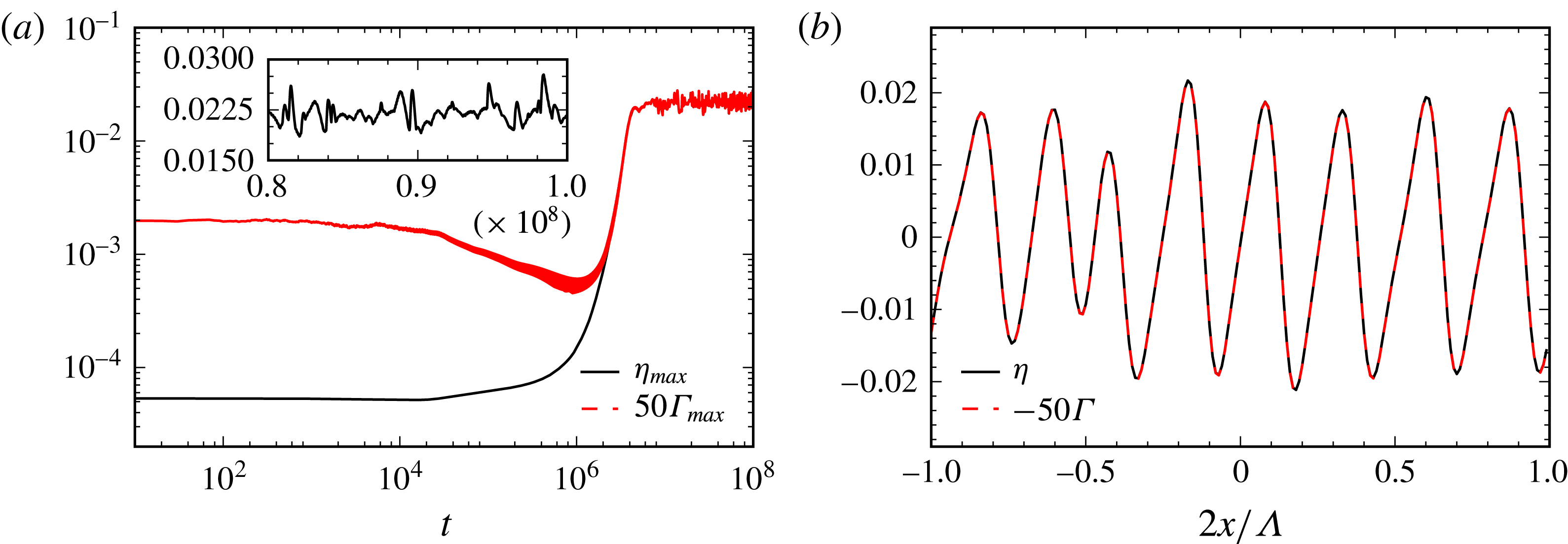
Such small-amplitude saturation solutions are found even with zero Bond number in the
 $R$
sector. The Bond number terms disappear from (6.1) and (6.2). In the latter, if the Marangoni number is of order one or less, for the long waves, the term with the second derivative of
 $\unicode[STIX]{x1D6E4}$
is much smaller than the term with the first derivative of
 $\unicode[STIX]{x1D6E4}$
, and the dominant balance is between the
 $\unicode[STIX]{x1D6E4}_{x}$
and the
 $\unicode[STIX]{x1D702}_{x}$
terms in equation (6.2) provided that the time scale is sufficiently large. This, similar to (6.6), implies the relation
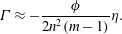 $$\begin{eqnarray}\unicode[STIX]{x1D6E4}\approx -\frac{\unicode[STIX]{x1D719}}{2n^{2}(m-1)}\unicode[STIX]{x1D702}.\end{eqnarray}$$
In the
 $R$
and
 $Q$
sectors this clearly implies that
 $\unicode[STIX]{x1D6E4}$
and
 $\unicode[STIX]{x1D702}$
are in anti-phase. (Note that the same relation is found for the normal modes of the linear theory given by (3.30). Also, in the limit of
 $m=n^{2}$
and
 $n\rightarrow \infty$
we recover the relation (6.6).) Substituting (6.15) into the kinematic equation (6.1) we obtain the Kuramoto–Sivashinsky equation
 $$\begin{eqnarray}\unicode[STIX]{x1D702}_{t}+\frac{n^{3}(m+n)}{3\unicode[STIX]{x1D713}}\unicode[STIX]{x1D702}_{xxxx}+\frac{\unicode[STIX]{x1D719}(n^{2}-m)Ma}{4\unicode[STIX]{x1D713}(m-1)}\unicode[STIX]{x1D702}_{xx}+sN_{1}\unicode[STIX]{x1D702}\unicode[STIX]{x1D702}_{x}=0.\end{eqnarray}$$
The characteristic scales (assuming that all other parameters except for
 $Ma$
are of order one including
 $m-1$
) become
 $L\sim Ma^{-1/2}$
,
 $N\sim Ma/L\sim Ma^{3/2}$
and
 $T\sim L^{4}\sim Ma^{-2}$
. Hence for
 $Ma\ll 1$
, the length scale is large, the time scale is even much larger, the amplitudes are small, and the previously assumed dominant balance in the surfactant equation is justified. With these scales, neglecting the term with
 $Bo$
in (6.1) in comparison with the fourth-derivative term is consistent if
 $Bo\ll L^{-2}$
, that is
 $Bo\ll Ma$
. (Neglecting the term with
 $Bo$
in (6.2) as compared to the term with
 $\unicode[STIX]{x1D702}_{x}$
leads to a weaker requirement,
 $|Bo|\ll (n+1)\unicode[STIX]{x1D719}sL/(n^{2}(m-n^{2}))$
.) By considerations similar to those which led to (6.14), we obtain a correction to (6.15) due to the initial conditions,
 $$\begin{eqnarray}\unicode[STIX]{x1D6E4}(t,x)=-\frac{\unicode[STIX]{x1D719}}{2n^{2}(m-1)}\unicode[STIX]{x1D702}(t,x)+\left(\unicode[STIX]{x1D6E4}(0,x-at)-\frac{\unicode[STIX]{x1D719}}{2n^{2}(m-1)}\unicode[STIX]{x1D702}(0,x-at)\right),\end{eqnarray}$$
where
 $a=2(m-1)n^{2}(n+1)s/\unicode[STIX]{x1D713}$
. For example, for
 $m=n=2$
, the relation (6.14) gives
 $\unicode[STIX]{x1D6E4}=-{\textstyle \frac{17}{4}}\unicode[STIX]{x1D702}$
for the large-time, permanent, saturated state. Thus we have two chaotic functions,
 $\unicode[STIX]{x1D702}$
and
 $\unicode[STIX]{x1D6E4}$
, which differ by just a constant factor. As an illustration, a numerical simulation (of the strongly nonlinear system) yields the time dependencies of
 $\unicode[STIX]{x1D702}_{max}$
and
 $\unicode[STIX]{x1D6E4}_{max}$
, figure 7(a), which show the saturation of instability, and the spatial profiles, figure 7(b), which are all in excellent agreement with the predictions. The present result of small-amplitude saturation is in marked contrast with our earlier findings (see Frenkel & Halpern Reference Frenkel and Halpern2006) that for the semi-infinite system, also with no gravity, no small-amplitude saturation is possible (which was also confirmed in the numerical simulations of Bassom et al.
Reference Bassom, Blyth and Papageorgiou2010; Kalogirou & Papageorgiou Reference Kalogirou and Papageorgiou2016).
(a) The maximum values of
 $\unicode[STIX]{x1D702}$
and
 $\unicode[STIX]{x1D6E4}$
as functions of time in the
 $R$
sector. Here
 $n=m=2$
,
 $s=1$
,
 $Ma=0.01$
,
 $Bo=0$
and
 $\unicode[STIX]{x1D6EC}=100\unicode[STIX]{x03C0}$
. The (linear scales) inset zooms in on
 $\unicode[STIX]{x1D702}_{max}$
for a later part of the run,
 $9\times 10^{7}<t<10^{8}$
. (b) Spatial profiles of
 $\unicode[STIX]{x1D702}$
and
 $\unicode[STIX]{x1D6E4}$
at the end time,
 $t=10^{8}$
, of the evolution pertaining to panel (a).
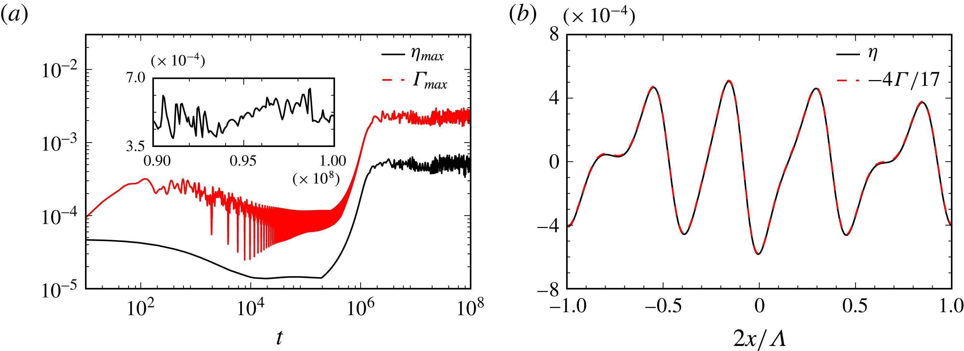
The above results have been obtained for the
 $R$
sector where the robust mode is unstable and the surfactant one is stable. To the contrary, in the
 $S$
sector, where the surfactant mode is unstable and the robust mode is stable for zero Bond number, there appears to be no small-amplitude saturation. Moreover, as is discussed in the next section, even the long-wave assumption may get violated after some time so that no long-wave solutions exist at large time.
In the
 $Q$
sector, for finite
 $m$
and
 $n$
, small negative
 $Bo$
, and assuming that
 $Ma$
is so small that the terms containing it can be discarded, we obtain again the decoupled Kuramoto–Sivashinsky equation, leading to
 $L\sim (-Bo)^{-1/2}$
,
 $N\sim n^{3}(m+n)/(3\unicode[STIX]{x1D713}L^{3}s)$
and
 $T\sim 3\unicode[STIX]{x1D713}L^{4}n^{-3}/(m+n)$
. We can see that the relation (6.15) holds here as well as in the
 $R$
sector. Such solutions belonging to the
 $Q$
sector are illustrated in figure 8. Note that
 $\unicode[STIX]{x1D6E4}\approx -55/32\unicode[STIX]{x1D702}$
, exactly as (6.15) predicts for
 $n=2$
and
 $m=5$
.
(a) Time dependence of the maximum values of
 $\unicode[STIX]{x1D702}$
and
 $\unicode[STIX]{x1D6E4}$
in the
 $Q$
sector. The parameter values are
 $n=2$
,
 $m=5$
,
 $s=1$
,
 $Ma=0.001$
,
 $Bo=-0.01$
and
 $\unicode[STIX]{x1D6EC}=200\unicode[STIX]{x03C0}$
. The (linear scales) inset zooms in on
 $\unicode[STIX]{x1D702}_{max}$
for a later part of the run,
 $8\times 10^{7}<t<10^{8}$
. (b) Spatial profiles of
 $\unicode[STIX]{x1D702}$
and
 $\unicode[STIX]{x1D6E4}$
at the end time,
 $t=10^{8}$
, of the evolution pertaining to (a).
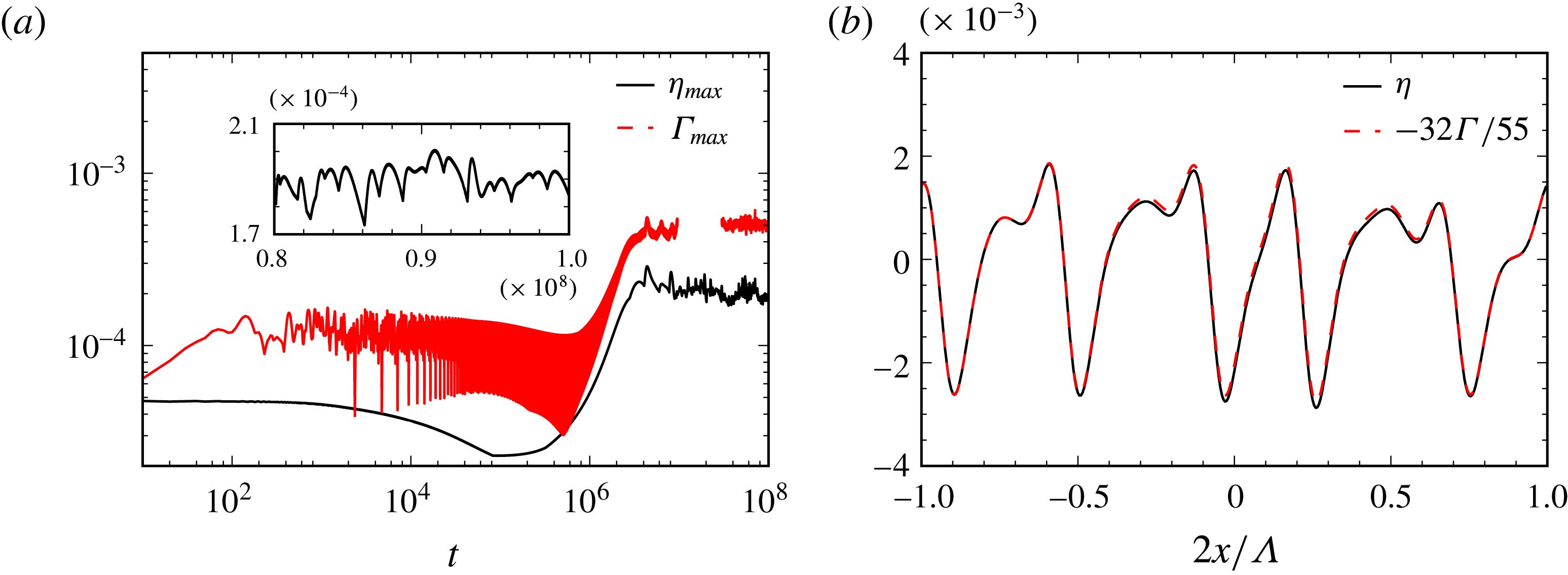
As we know in the
 $S$
sector the robust modes are unstable provided that the Bond number is negative and below the threshold given by (4.14). They still saturate with small amplitude like in the
 $R$
and
 $Q$
sectors. The difference is that
 $\unicode[STIX]{x1D6E4}$
and
 $\unicode[STIX]{x1D702}$
are in phase as opposed to anti-phase. For example, in the cases where the Marangoni number is essentially zero, we have the Kuramoto–Sivashinsky equation (6.1) with a destabilizing gravity term. This leads to small-amplitude saturation of the Rayleigh–Taylor instability. Similar saturation was found e.g. in Babchin et al. (Reference Babchin, Frenkel, Levich and Sivashinsky1983) but for
 $n=\infty$
. (Note, however, that the saturation of the Rayleigh–Taylor instability in the finite channels has not been demonstrated before the present study.) The surfactant in this case plays no dynamical role, and is just advected passively by the flow.
6.2 Nonlinear saturation in the
$S$
sector with linearly unstable surfactant modes

In the previous subsection we established that unstable robust modes saturate with the amplitudes of both
 $\unicode[STIX]{x1D702}$
and
 $\unicode[STIX]{x1D6E4}$
being small. To the contrary, in the
 $S$
sector, there appears to be no small-amplitude saturation of the linearly unstable surfactant mode. (Recall that the surfactant modes are linearly stable in the
 $R$
and
 $Q$
sectors.) However, it is possible that the saturated
 $\unicode[STIX]{x1D702}$
amplitude is still small while the saturated
 $\unicode[STIX]{x1D6E4}$
is not small. For such regimes, as was noted above, the linear transport equation (6.2) acquires a nonlinear term and thus takes the form
 $$\begin{eqnarray}\displaystyle & & \displaystyle \unicode[STIX]{x1D6E4}_{t}+\frac{(n+1)\unicode[STIX]{x1D719}}{\unicode[STIX]{x1D713}}s[\unicode[STIX]{x1D702}(1+\unicode[STIX]{x1D6E4})]_{x}+\frac{2(m-1)n^{2}(n+1)s}{\unicode[STIX]{x1D713}}\unicode[STIX]{x1D6E4}_{x}-\frac{n(m+n^{3})Ma}{\unicode[STIX]{x1D713}}[\unicode[STIX]{x1D6E4}_{x}(1+\unicode[STIX]{x1D6E4})]_{x}\nonumber\\ \displaystyle & & \displaystyle \quad -\,\frac{n^{2}(n^{2}-m)Bo}{2\unicode[STIX]{x1D713}}\unicode[STIX]{x1D702}_{xx}+\frac{n^{2}(n^{2}-m)}{2\unicode[STIX]{x1D713}}\unicode[STIX]{x1D702}_{xxxx}=0.\end{eqnarray}$$
Note that a nonlinear term containing Marangoni number has been included, as it may be comparable with the
 $s$
term, since the extra differentiation in the former can be balanced by the smallness of
 $\unicode[STIX]{x1D702}$
in the latter.
Moreover, even the long-wave assumption may get violated after some time so that no long-wave solutions exist at large time. As an example, the run corresponding to figure 9(a) starts with a very long-wave sinusoidal initial condition, but later, as shown in figure 9(b), a short-wave disturbance appears on a limited part of the profiles. As time goes on, the amplitude and the extent of the disturbance grow (see figure 9
c), and on the post-saturation stage (see figure 10), we have small amplitude
 $\unicode[STIX]{x1D702}$
but
 $\unicode[STIX]{x1D6E4}$
of order one, and the characteristic length of the pulses is not large. Then, even the lubrication-approximation assumptions are not satisfied. This non-applicability of the lubrication approximation seems to be a general feature for the
 $S$
sector. For example, if we take the Bond number sufficiently negative so that there are unstable robust modes along with the unstable surfactant ones, we get results similar to the ones shown in figure 11. We note that for these ‘deeply robust’ regimes the number of
 $\unicode[STIX]{x1D6E4}$
pulses appears to be different from that of
 $\unicode[STIX]{x1D702}$
pulses. This contrasts with the purely surfactant mode regimes, and the robust surfactant regimes with a smaller negative value of the Bond number. (We also note that the amplitude of fluctuations of
 $\unicode[STIX]{x1D702}_{max}$
and
 $\unicode[STIX]{x1D6E4}_{max}$
in the post-saturation state may change with the number of pulses on the computation interval. This occurs due to coalescences of pulses and the emergence of new pulses, similar to such phenomena observed for a different strongly nonlinear equation in Kerchman & Frenkel (Reference Kerchman and Frenkel1994).)
(a) The maximum values of
 $\unicode[STIX]{x1D702}$
and
 $\unicode[STIX]{x1D6E4}$
as functions of time in the
 $S$
sector, with
 $n=2$
,
 $m=1/2$
,
 $s=1$
,
 $Ma=10^{-2}$
,
 $Bo=0$
and
 $\unicode[STIX]{x1D6EC}=20\unicode[STIX]{x03C0}$
. (b)
 $\unicode[STIX]{x1D702}$
and (c)
 $\unicode[STIX]{x1D6E4}$
profiles near the moment when small-scale disturbances appear if large scale but small-amplitude initial conditions are used. Note that only the right half of the spatial domain is shown, where the small scales first appear.
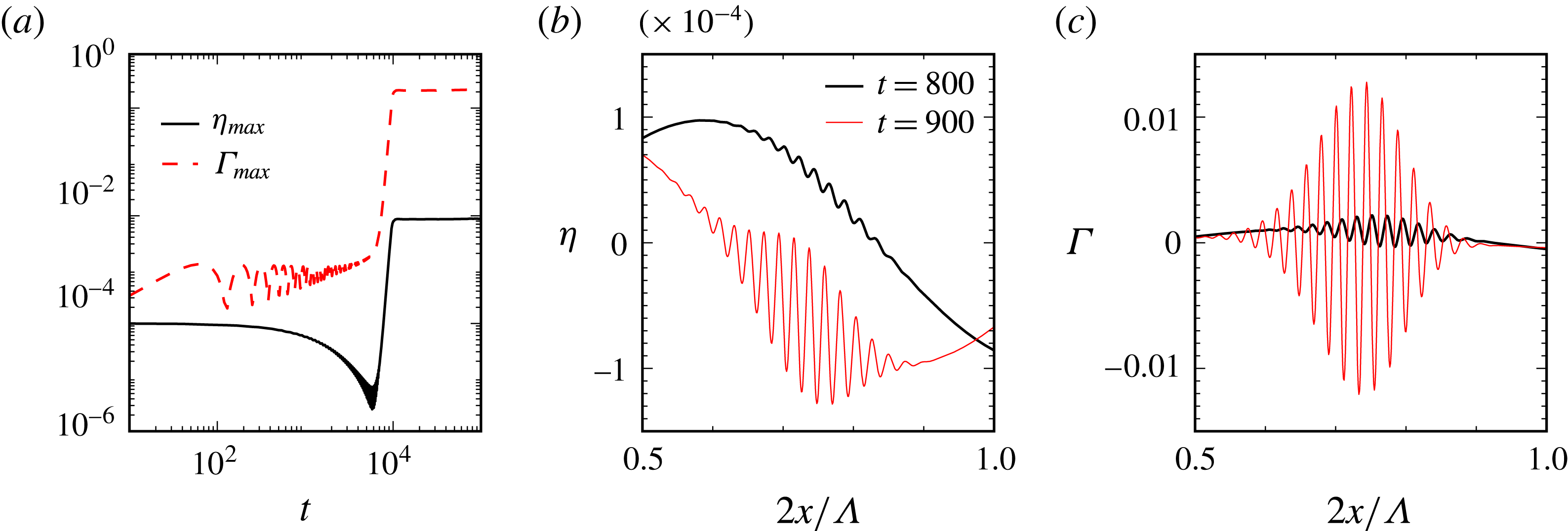
Small amplitude
 $\unicode[STIX]{x1D702}$
and large amplitude
 $\unicode[STIX]{x1D6E4}$
profiles at the end time,
 $t=10^{5}$
, of the evolution corresponding to figure 9(a).
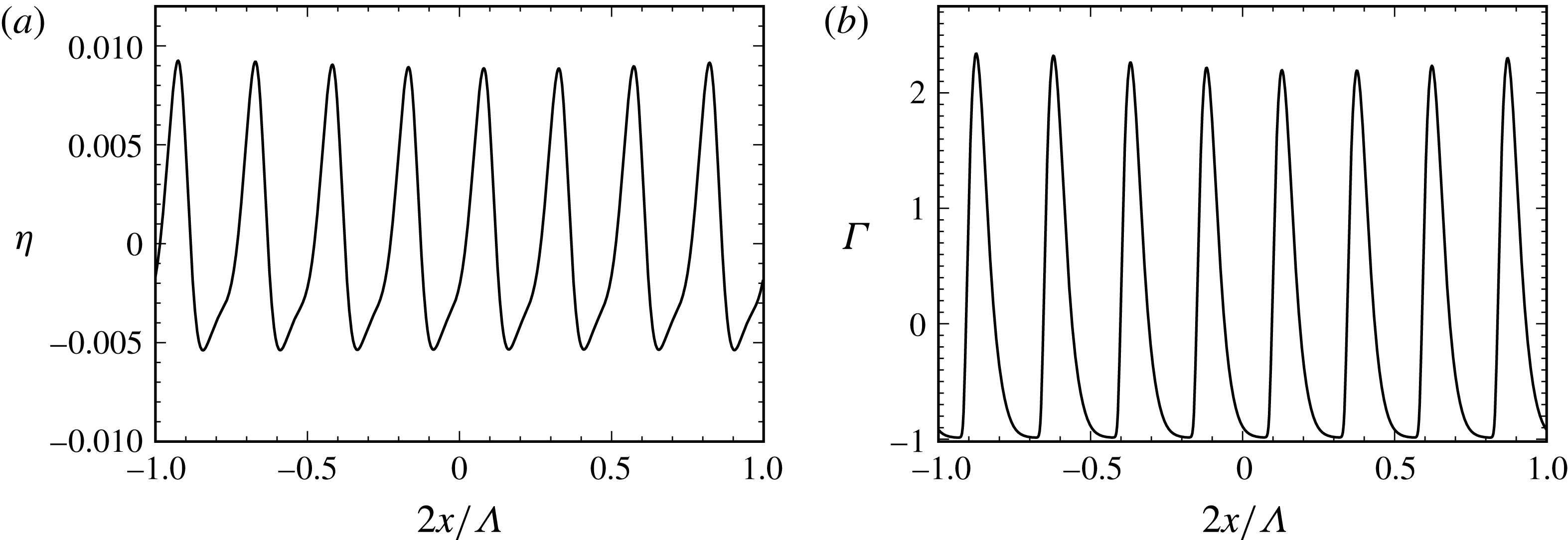
(a) Evolution of the maximum amplitude of
 $\unicode[STIX]{x1D702}$
and
 $\unicode[STIX]{x1D6E4}$
for the same parameter values as in the preceding two figures (thus in the
 $S$
sector), with the exception that
 $Bo=-0.5$
here. (b) Small amplitude
 $\unicode[STIX]{x1D702}$
and large amplitude
 $\unicode[STIX]{x1D6E4}$
at the end time,
 $t=10^{5}$
.
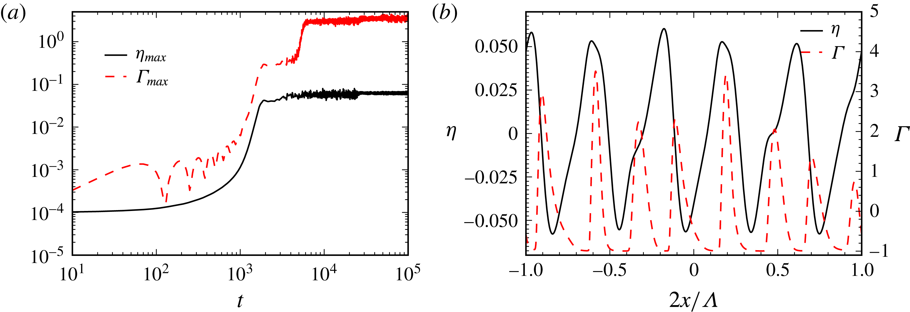
7 Summary and discussion
This study concerned the linear and nonlinear stages of evolution of initially small disturbances of the horizontal two-fluid Couette flow (with top-to-bottom aspect ratio
 $n$
and viscosity ratio
 $m$
) in the presence of surfactants and gravity, and with negligible inertia (figure 1). For any flow with
 $n<1$
, it is described as one with
 $n>1$
in a new coordinate system obtained by reversing the (spanwise)
 $z$
-axis direction. Therefore, without loss of generality, we consider the flows with
 $n\geqslant 1$
. The lubrication approximation yields two coupled strongly nonlinear evolution equations for the interface thickness and the insoluble surfactant concentration. These equations take a weakly nonlinear form when the amplitudes of disturbances are small, but finite. The onset of instability is investigated by linearizing (for the infinitesimal disturbances) these evolution equations and applying, as usual, the normal-mode analysis.
The dispersion relation for the increment (a complex eigenvalue which determines the real growth rate and the phase velocity) of the linear instability is found to be a quadratic equation whose coefficients depend on the interfacial shear rate, the aspect and viscosity ratios, the Marangoni number and the Bond number. As introduced in HF for the case of no gravity, the subdivision of the
 $n\geqslant 1$
part of the
 $(n,m)$
-plane into the three sectors – called here the
 $Q$
sector, in which
 $m>n^{2}>1$
; the
 $R$
sector, characterized by
 $1<m<n^{2}$
; and the
 $S$
sector,
 $m<1$
(figure 2) – turns out to be useful even in the presence of gravity.
The growth rate dependence on the wavenumber, being the real part of the solution to the quadratic equation, has two single-valued continuous branches, called the robust branch and the surfactant one. Correspondingly, for each wavenumber, there is a single robust normal mode that exists even when
 $Ma=0$
and
 $s=0$
, and a single surfactant normal mode that vanishes when
 $Ma\downarrow 0$
, and we speak of the two branches (sets) of modes. The expressions for the growth rates for the base flows with a non-zero shear rate
 $s$
differ from those for a stagnant base two-layer system.
For
 $s\neq 0$
, the growth rate for the robust branch (see (4.3)) is the sum of two terms, which are both independent of
 $s$
: a Marangoni term (which equals the growth rate due to the surfactant in the absence of gravity, first found in Frenkel & Halpern (Reference Frenkel and Halpern2002)), and a Bond term (which gives the well-known growth rate of the Rayleigh–Taylor instability of the flow with no surfactants). The Marangoni term is negative in the
 $S$
and
 $Q$
sectors and positive in the
 $R$
sector. The Bond term (with its negative sign included) clearly increases when the Bond number decreases. Therefore, the instability sets in when the Bond number is less than some threshold value denoted
 $Bo_{cL}$
. In the
 $Q$
and
 $S$
sectors, where the Marangoni term is negative, the surfactant acts on the robust modes in a stabilizing way, so
 $Bo_{cL}<0$
, while in the
 $R$
sector, the surfactant action has a destabilizing character and hence
 $Bo_{cL}>0$
. The ratio of the threshold Bond number to the Marangoni number, being independent of the base shear rate
 $s$
, varies with the two remaining variables, the aspect ratio
 $n$
and the viscosity ratio
 $m$
, only (figure 3).
In contrast to the robust modes, the growth rate for the surfactant branch with
 $s\neq 0$
(see (4.5)) has no purely Bond term; the leading term is purely Marangoni, not containing the Bond number at all; and the higher-order terms, if they have the Bond number as a factor, always contain some Marangoni number factor as well. These surfactant modes are stable in the
 $Q$
and
 $R$
sectors and unstable in the
 $S$
sector. Thus, in the
 $S$
sector, a finite band of the long-wave surfactant modes, somewhat surprisingly, are unstable even for arbitrarily large Bond number (albeit the band width is expected to decrease as gravity grows stronger). Thus, no amount of gravity, however strong, can completely stabilize the surfactant instability in the
 $S$
sector.
On the other hand, in the
 $Q$
sector, the surfactant can stabilize the Rayleigh–Taylor instability. Only the robust branch needs to be stabilized since the surfactant one is stable independent of the Bond number (see 4.5). For example, the flow with
 $n=2$
,
 $m=5$
and
 $Bo=-0.015$
is Rayleigh–Taylor unstable in the absence of surfactant. But in the presence of surfactant, such that, say,
 $Ma=0.1$
, the flow is stable according to (4.3). This value of the Bond number corresponds to
 $(\unicode[STIX]{x1D70C}_{2}-\unicode[STIX]{x1D70C}_{1})gd_{1}^{2}=0.015\unicode[STIX]{x1D70E}_{0}$
in view of (3.6), that is, for
 $\unicode[STIX]{x1D70E}_{0}=10$
(in cgs units),
 $(\unicode[STIX]{x1D70C}_{2}-\unicode[STIX]{x1D70C}_{1})gd_{1}^{2}=0.15$
. For the Earth’s gravity,
 $g\approx 10^{3}$
, and
 $\unicode[STIX]{x1D70C}_{2}-\unicode[STIX]{x1D70C}_{1}\sim O(1)$
, this means the thickness
 $d_{1}\sim 10^{-2}~\text{cm}$
, a rather thin film. But, under the conditions of microgravity, with (say)
 $g\sim 10^{-1}$
, the bottom layer is much thicker,
 $d_{1}\sim 1~\text{cm}$
. (Even with the Earth’s gravity, the film thickness is
 $d_{1}\sim 10^{-1}~\text{cm}$
if the densities are almost equal,
 $\unicode[STIX]{x1D70C}_{2}-\unicode[STIX]{x1D70C}_{1}\sim 10^{-2}$
.) It is remarkable that the interfacial surfactant can completely suppress the Rayleigh–Taylor instability under quite realistic physical conditions.
The lubrication approximation is sufficient for finding the results, including increments, at the leading order and also in the next-order correction. For the robust mode, the leading order of the increment determines the wave velocity which turns out to be independent of the wavenumber
 $\unicode[STIX]{x1D6FC}$
and hence can be eliminated by using the co-moving reverence frame. To find the first truly non-zero term of the wave velocity, scaling as
 $\unicode[STIX]{x1D6FC}^{2}$
, one needs the first post-lubrication corrections to the governing equations (as found in appendix B of Frenkel & Halpern Reference Frenkel and Halpern2016), whereas the lubrication-theory increment correction gives the leading-order growth rate.
For the case of equal viscosities,
 $m=1$
, i.e. on the boundary between the
 $R$
and
 $S$
sectors, the gravitational effects are absent at the leading order, and so, as was found in Frenkel & Halpern (Reference Frenkel and Halpern2002), both growth rates scale as
 $\unicode[STIX]{x1D6FC}^{3/2}$
(5.57). The correction to them, proportional to
 $-\unicode[STIX]{x1D6FC}^{2}Bo$
, is the same for both modes (5.60).
For the case with no base flow, i.e. with
 $s=0$
, both modes are stable if the Bond number is positive, but one of the modes is unstable if the Bond number is negative. This is essentially the Rayleigh–Taylor instability of a stagnant system modified by the surfactant.
The eigenfunction amplitudes, including those of the surfactant concentration
 $G$
(where the arbitrary interface deviation amplitude
 $h$
is taken to be real and positive), the velocities and pressures, are determined as well. This can be done using the eigenvectors of the system for
 $G$
and
 $h$
. However, we have used also a different way, linearizing the primitive governing equations (rather than the two evolution equations derived from them) and using the method of undetermined coefficients, which has advantages in uncovering the physical mechanisms of instability for the two modes.
We suggested that in the inertialess settings, the vorticity lacks the dynamic significance which was shown by Charru & Hinch (Reference Charru and Hinch2000) for a surfactantless case of the Yih instability, whose very existence depends on inertia. Thus, in contrast to the case of Yih instability, vorticity does not appear to be a suitable agent for the mechanism of the surfactant instability. Wei (Reference Wei2005) showed that under certain conditions, without gravitational effects, there is a correlation of stability of normal modes with
 $\unicode[STIX]{x1D703}_{\unicode[STIX]{x1D714}}$
, the phase shift between the interfacial vorticity and the interfacial displacement. Namely,
 $\unicode[STIX]{x1D703}_{\unicode[STIX]{x1D714}}$
being in the interval
 $(0,\unicode[STIX]{x03C0})$
corresponds to instability while
 $\unicode[STIX]{x1D703}_{\unicode[STIX]{x1D714}}$
within the interval
 $(-\unicode[STIX]{x03C0},0)$
corresponds to stability. However, we showed that, under the same conditions, except for the Bond number being non-zero, this correspondence does not necessarily hold. For example, figure 4 shows that the growth rate changes from negative to positive as the Marangoni number grows, but the vorticity-interface phase shift remains in the same interval
 $(0,\unicode[STIX]{x03C0})$
all along, thus for both the stable and unstable flows. This is related to the lack of any significant role of vorticity for instability in the absence of inertial effects, with or without gravitational effects.
To uncover the mechanisms of instability for the two modes, we considered the case of large thickness ratio and used the mass conservation laws in their integral forms (similar to Charru & Hinch Reference Charru and Hinch2000). The growth/decay mechanism for the robust branch is as follows: the leading-order disturbance flow is the same as in Yih (Reference Yih1967) and leads to the same, purely imaginary, increment. This flow is found from physical considerations as in Charru & Hinch (Reference Charru and Hinch2000), using the fact that the thick-layer disturbances uncouple in the case of the large aspect ratio. The surfactant transport is determined by the base velocity at the perturbed interface. As a result, the surfactant wave of the normal mode must propagate either in anti-phase, for
 $m>1$
, or in phase, for
 $m<1$
, with the interface. The Marangoni tangential stress exerted by the surfactant drives a correction flow in the thin layer whose horizontal velocity is
 $-90^{\circ }$
out-of-phase with the surfactant. (This holds for all elevations, since the vertical profile of this velocity is linear, and thus it has the same sign at all elevations.) Thus, this velocity is either
 $90^{\circ }$
, for
 $m>1$
, or
 $-90^{\circ }$
, for
 $m<1$
, out of phase with the interface. For
 $m>1$
, this leads to a net outflow for the half-period part of the thin layer with the thickness minimum at the interval midpoint, which means instability for the normal mode; and for
 $m<1$
, the velocity is reversed, which yields stability.
The surfactant branch corresponds to the Marangoni stresses playing a role already at the leading order of disturbances (in contrast to their correction role for the robust branch). The leading-order flow disturbance in the thick layer is still the same as that for the robust mode. We find that the Marangoni stress must cancel the viscous tangential stress of the thick layer at the interface. As a result, the surfactant phase shift with respect to the interface is
 $90^{\circ }$
for
 $m>1$
and
 $-90^{\circ }$
for
 $m<1$
. On the other hand, the surfactant flux, the product of the base concentration and the thin-layer base velocity at the perturbed interface, is always in phase with the interface. Hence, the surfactant flux is out of phase with the surfactant wave,
 $90^{\circ }$
for
 $m>1$
and
 $-90^{\circ }$
for
 $m<1$
. Thus, considering the half-period interval of the wave with the maximum positive net influx through its end points, the surfactant concentration is minimum at the midpoint for
 $m>1$
, but the magnitude of this minimum gradually decreases, which means stability. In contrast, for
 $m<1$
the surfactant concentration is maximum at the midpoint, which grows because of the positive net influx of the surfactant, and this corresponds to instability.
With no gravity, small-amplitude nonlinear saturation of the surfactant instability is possible (figure 7), in contrast to the semi-infinite case studied by Frenkel & Halpern (Reference Frenkel and Halpern2006). For non-zero Bond number, the small-amplitude saturation in the
 $Q$
sector is seen in figure 8(a). It also occurs along the border between the
 $R$
and
 $Q$
sectors, where
 $m=n^{2}$
, for
 $Bo<0$
(figure 6
a).
For certain ranges of
 $(m,n)$
, in the
 $R$
and
 $Q$
sectors, the interface is governed by a decoupled Kuramoto–Sivashinsky equation, whose solution provides a source term for the linear convection–diffusion equation of the surfactant. When diffusion is negligible, the surfactant equation has an analytic solution. As a result, the surfactant wave is as chaotic as the interface; however, the ratio of the two waves is constant at sufficiently large times such that the saturated state has been reached (figures 6
b, 7
b and 8
b). These analytical predictions are confirmed by the full numerical solution of the nonlinear evolution equations.
In contrast, we have never seen the small-amplitude saturation in the
 $S$
sector,
 $m<1$
. Instead, numerical results show that the instability saturates with only the interface disturbances being small amplitude but the surfactant ones large (figures 9 and 11). However, the final characteristic length scale of these solutions is not as large as is required by the lubrication approximation (figures 10
b and 11
b). To the best of our knowledge, the only other simulations for the case of finite aspect ratio, even with zero gravity, were performed in Blyth & Pozrikidis (Reference Blyth and Pozrikidis2004b
). They were limited to the
 $S$
sector and small computational intervals. The saturation that they observed was not small amplitude, and we checked that if extended to sufficiently large intervals, the evolution leads to a characteristic length scale being small, and thus not consistent with the lubrication approximation. The question whether such partly weakly and partly strongly nonlinear saturated regimes are real may be decided by a future non-lubrication theory. Also, the inertial effects could be included, for example, similar to Frenkel & Halpern (Reference Frenkel and Halpern2005). The three-dimensional disturbances could be considered similar to Frenkel & Halpern (Reference Frenkel and Halpern2000).
Appendix A. Eigenfunctions: velocities and pressure
Provided
 $s\neq 0$
the velocities are as follows. For the surfactant branch, the real part of the (bottom layer) horizontal velocity component
 $u_{1}$
, to its leading order
 $\unicode[STIX]{x1D6FC}^{0}$
, is
 $$\begin{eqnarray}\text{Re}(u_{1})=-hs\frac{(m-1)}{(m-n^{2})}(z+1)(3z+1);\end{eqnarray}$$
the imaginary part of
 $u_{1}$
, to its leading order
 $\unicode[STIX]{x1D6FC}^{1}$
, is
 $$\begin{eqnarray}\displaystyle \text{Im}(u_{1}) & = & \displaystyle \unicode[STIX]{x1D6FC}h\frac{1}{(m-n^{2})}(z+1)\left\{Ma\frac{(n-1)}{2(m-1)n}[3m(n+1)(z-1)+4m+3mn+n^{3}]\right.\nonumber\\ \displaystyle & & \displaystyle -\left.Bo\frac{n^{2}}{6}(3z+1)\right\}.\end{eqnarray}$$
The real part of the (top layer) velocity component
 $u_{2}$
, to its leading order
 $\unicode[STIX]{x1D6FC}^{0}$
, is
 $$\begin{eqnarray}\text{Re}(u_{2})=-hs\frac{(m-1)}{m(m-n^{2})}(z-n)(3z-n);\end{eqnarray}$$
the imaginary part of
 $u_{2}$
, to its leading order
 $\unicode[STIX]{x1D6FC}^{1}$
, is
 $$\begin{eqnarray}\displaystyle \text{Im}(u_{2}) & = & \displaystyle -\unicode[STIX]{x1D6FC}h\frac{1}{(m-n^{2})}(z-n)\!\left\{\!Ma\frac{(n-1)}{2(m-1)n^{2}}[-3(z+n)n(n+1)+(m+3n^{2}+4n^{3})]\right.\nonumber\\ \displaystyle & & \displaystyle \left.+\,\frac{Bo}{6}(3z-n)\right\}.\end{eqnarray}$$
(Note that
 $h=$
for
 $m=n^{2}$
. For this case, the velocities can be expressed in terms of
 $G$
rather than
 $h$
, in the same way as (A 17) and (A 18) below.)
For the robust branch, the real part of the (bottom-layer horizontal velocity component)
 $u_{1}$
, to its leading order
 $\unicode[STIX]{x1D6FC}^{0}$
, is
 $$\begin{eqnarray}\text{Re}(u_{1})=-hs\frac{(m-1)}{\unicode[STIX]{x1D713}}(z+1)[3(m-n^{2})(z-1)+4(m+n^{3})];\end{eqnarray}$$
the imaginary part of
 $u_{1}$
, to its leading order
 $\unicode[STIX]{x1D6FC}^{1}$
, is
 $$\begin{eqnarray}\displaystyle \text{Im}(u_{1}) & = & \displaystyle \unicode[STIX]{x1D6FC}h\frac{1}{2\unicode[STIX]{x1D713}}(z+1)\left\{Ma\frac{\unicode[STIX]{x1D711}}{(m-1)n}[3m(n+1)(z-1)+(4m+3nm+n^{3})]\right.\nonumber\\ \displaystyle & & \displaystyle \left.+\,Bon^{2}[(3m+4nm+n^{2})(z-1)+4m(n+1)]\right\}.\end{eqnarray}$$
The real part of
 $u_{2}$
, to its leading order
 $\unicode[STIX]{x1D6FC}^{0}$
, is
 $$\begin{eqnarray}\text{Re}(u_{2})=-hs\frac{(m-1)}{m\unicode[STIX]{x1D713}}(z-n)[3(m-n^{2})(z+n)+4(m+n^{3})];\end{eqnarray}$$
the imaginary part of
 $u_{2}$
its leading order
 $\unicode[STIX]{x1D6FC}^{1}$
, is
 $$\begin{eqnarray}\displaystyle \text{Im}(u_{2}) & = & \displaystyle \unicode[STIX]{x1D6FC}h\frac{1}{2\unicode[STIX]{x1D713}}(z-n)\left\{Ma\frac{\unicode[STIX]{x1D711}}{(m-1)n^{2}}[3n(n+1)(z+n)-(m+3n^{2}+4n^{3})]\right.\nonumber\\ \displaystyle & & \displaystyle +\,\left.Bo[-(m+4n+3n^{2})(z+n)+4(n+1)n^{2}]\right\}.\end{eqnarray}$$
For the special case
 $m=1$
, the leading-order velocities are
 $$\begin{eqnarray}\displaystyle & \displaystyle u_{1}=\pm \unicode[STIX]{x1D6FC}^{1/2}(1-\text{i})h\left(2Mas\frac{n^{2}}{(n+1)^{3}(n-1)}\right)^{1/2}(z+1)[3(z-1)+(n^{2}-n+4)],\qquad & \displaystyle\end{eqnarray}$$
 $$\begin{eqnarray}\displaystyle & \displaystyle u_{2}=\mp \unicode[STIX]{x1D6FC}^{1/2}(1-\text{i})h\left(2Mas\frac{1}{(n+1)^{3}(n-1)}\right)^{1/2}(z-n)[-3n(z+n)+(4n^{2}-n+1)], & \displaystyle \nonumber\\ \displaystyle & & \displaystyle\end{eqnarray}$$
with the upper/lower signs for the growing/decaying modes, respectively. The next-order corrections are
 $$\begin{eqnarray}\displaystyle & \displaystyle u_{1}^{c}=\unicode[STIX]{x1D6FC}\text{i}hBo\frac{n^{2}}{6(n+1)^{3}(n-1)}(z+1)[3(z-1)(n^{2}+2n-1)+2(n^{2}+5n-2)],\qquad & \displaystyle\end{eqnarray}$$
 $$\begin{eqnarray}\displaystyle & \displaystyle u_{2}^{c}=\unicode[STIX]{x1D6FC}\text{i}hBo\frac{1}{6(n+1)^{3}(n-1)}(z-n)[3(z+n)(-n^{2}+2n+1)+2n(2n^{2}-5n-1)]. & \displaystyle \nonumber\\ \displaystyle & & \displaystyle\end{eqnarray}$$
(Note that the corrections for the growing mode are the same as for the decaying one.)
Considering the special case
 $s=0$
and
 $Bo=0$
(that implies that the leading-order disturbances vanish, along with the base flow), the horizontal velocities are as follows. For the surfactant branch, the bottom-layer horizontal velocity is
 $$\begin{eqnarray}u_{1}=\text{i}2h\frac{(m+n^{3})}{n(m-n^{2})\unicode[STIX]{x1D713}}(z+1)[3mn(n+1)(z-1)+4m+3mn+n^{3}]\end{eqnarray}$$
while for the top layer, it is
 $$\begin{eqnarray}u_{2}=-\text{i}2h\frac{(m+n^{3})}{n(m-n^{2})\unicode[STIX]{x1D713}}(z-n)[-3n(n+1)(z+n)+m+3n^{2}+4n^{3}].\end{eqnarray}$$
For the robust branch, the horizontal velocity in the bottom layer is
 $$\begin{eqnarray}u_{1}=-\text{i}\frac{2h(m+n)n^{2}\unicode[STIX]{x1D6FC}^{2}}{3(m-n^{2})\unicode[STIX]{x1D713}}(z+1)[3(n+1)(z-1)+4m+3mn+n^{3}]\end{eqnarray}$$
and for the top layer, it is
 $$\begin{eqnarray}u_{2}=\text{i}\frac{2h(m+n)n\unicode[STIX]{x1D6FC}^{2}}{3(m-n^{2})\unicode[STIX]{x1D713}}(z-n)[-3n(n+1)(z+n)+m+3n^{2}+4n^{3}].\end{eqnarray}$$
For the special case
 $s=0$
and
 $Bo\neq 0$
, the horizontal velocities in terms of
 $h$
and
 $G$
are
 $$\begin{eqnarray}\displaystyle u_{1} & = & \displaystyle \text{i}\unicode[STIX]{x1D6FC}\frac{1}{2\unicode[STIX]{x1D713}}(z+1)\{-2MaGn[3m(n+1)(z-1)+(4m+3nm+n^{3})]\nonumber\\ \displaystyle & & \displaystyle +\,Bohn^{2}[(3m+4nm+n^{2})(z-1)+4m(n+1)]\}\end{eqnarray}$$
and
 $$\begin{eqnarray}\displaystyle u_{2} & = & \displaystyle \text{i}\unicode[STIX]{x1D6FC}\frac{1}{2\unicode[STIX]{x1D713}}(z-n)\{-2MaGn[3n(n+1)(z+n)-(m+3n^{2}+4n^{3})]\nonumber\\ \displaystyle & & \displaystyle +\,Boh[-(m+4n+3n^{2})(z+n)+4(n+1)n^{2}]\}.\end{eqnarray}$$
These velocities can be written in terms of
 $h$
only by using the expression for
 $G$
in terms of
 $h$
from (4.13), in which the two different values of
 $\unicode[STIX]{x1D6FE}$
given by (3.34) correspond to the two different normal modes for the case
 $s=0$
and
 $Bo\neq 0$
.
Using these horizontal velocities, the vertical velocities for the two branches are obtained by integrating equation (3.3):
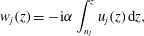 $$\begin{eqnarray}w_{j}(z)=-\text{i}\unicode[STIX]{x1D6FC}\int _{n_{j}}^{z}u_{j}(z)\,\text{d}z,\end{eqnarray}$$
(where
 $n_{1}=-1$
and
 $n_{2}=n$
, defined above for (3.2)). The pressures of the two branches can be readily obtained using (3.1), which yields
 $$\begin{eqnarray}\text{i}\unicode[STIX]{x1D6FC}p_{j}=m_{j}D^{2}u_{j}.\end{eqnarray}$$