1 Introduction
Swirling flows can frequently be observed in nature and occur in a wide variety of fluid devices for engineering applications. In the atmosphere, vigorous phenomena of meteorological relevance are associated with the accelerated swirling motion of large masses of air, tornadoes being a notable example (Rotunno Reference Rotunno2013). In gas turbine combustors, swirling jets generate reverse flow regions near the nozzle exit to stabilize the flame (Lilley Reference Lilley1977; Candel et al. Reference Candel, Durox, Schuller, Bourgouin and Moeck2014). Moreover, turbulent mixers, agricultural spraying machines, whirlpools and cyclone separators work on the principle of swirling jets increasing the spreading rate with rapid mixing of the jet fluid with its surroundings.
A swirling jet is obtained by imparting azimuthal momentum to an axial jet flow using a swirl generator, such as vanes (Harvey Reference Harvey1962), axial–tangential fluid entry (Chigier & Chervinsky Reference Chigier and Chervinsky1967), rotating inlet tubes (Billant, Chomaz & Huerre Reference Billant, Chomaz and Huerre1998; Örlü & Alfredsson Reference Örlü and Alfredsson2008) or rotating perforated plates (Rose Reference Rose1962). A comprehensive review of swirl flows is given in a monograph by Gupta, Lilley & Syred (Reference Gupta, Lilley and Syred1984), where the swirling motion is demonstrated to affect both the mean flow field properties and the large-scale organization of the unsteady fluctuations. Furthermore, in the case of inert jets, the swirl imparted to the flow strongly enhances the jet spreading rate, mass entrainment rate, and momentum growth rate.
Swirling jets experience an adverse pressure gradient along the jet axis due to jet broadening and the conservation of momentum. Opposed to axisymmetric jets without swirl, it can be shown (Childs Reference Childs2010) that in the presence of swirl the radial equilibrium equation also requires a minimum of pressure on the jet axis since a radial pressure gradient is associated with the tangential velocity.
The swirling regime is determined by the amount of swirl (viz tangential momentum) imparted to the flow compared to the axial momentum. The ratio of axial flux of angular momentum to the product of the axial flux of axial momentum times the radius of the nozzle (
 $D/2$
) is referred to as the swirl number
 $S$
and is the most commonly adopted expression quantifying the degree of swirl. A practical approximation consists in expressing the swirl number in terms of the ensemble average of the axial and azimuthal velocity components
 $u$
and
 $u_{\unicode[STIX]{x1D717}}$
only (Toh, Honnery & Soria Reference Toh, Honnery and Soria2010):
 $$\begin{eqnarray}\displaystyle S=\frac{2\displaystyle \int _{0}^{\infty }\bar{u}\bar{u}_{\unicode[STIX]{x1D717}}r^{2}\,\text{d}r}{D\displaystyle \int _{0}^{\infty }(\bar{u}^{2}-\bar{u}_{\unicode[STIX]{x1D717}}^{2}/2)r\,\text{d}r}, & & \displaystyle\end{eqnarray}$$
where the overbar refers to ensemble-averaged quantities.
Jet mean spreading rate, entrainment and centreline velocity decay are all enhanced as the swirl number increases (see e.g. Park & Shin Reference Park and Shin1993). Two distinct regimes are noted: low swirl (
 $S<0.5$
) and high swirl (
 $S>0.6$
). In the latter case, the stronger adverse axial pressure gradient affects the near-field development of the jet along radial and axial directions, in turn leading to a flow recirculation zone close to the nozzle exit. This phenomenon is associated with the vortex breakdown mechanism (Lucca-Negro & O’Doherty Reference Lucca-Negro and O’Doherty2001), which was first observed on delta wing vortices by (Lambourne & Bryer Reference Lambourne and Bryer1962), and could be represented as giving the impression that the fluid has to comply with the surface of an imaginary body of revolution placed at the vortex (i.e. the jet) axis (Harvey Reference Harvey1962).
The unsteady flow organization of swirling jets develops under the effect of a shear layer composed of both azimuthal (as in an axisymmetric jet without swirl) and axial components (driven by the azimuthal component of the jet exit velocity). The azimuthal component of the shear layer introduces shear-induced instabilities of Kelvin–Helmholtz type (Kelvin Reference Kelvin1871). Due to the imparted swirl, the axial component can result in an unstable radial stratification of the angular momentum, which leads to centrifugal instability (Rayleigh Reference Rayleigh1917) when the circulation decreases outwards (Rayleigh’s inviscid criterion is a necessary and sufficient condition for instability of inviscid rotating flows). Chanaud (Reference Chanaud1965) first observed such three-dimensional oscillations in the jet structure. Syred & Beér (Reference Syred and Beér1974) hypothesized that the flow field may not be axisymmetric and that after vortex breakdown, the flow region near the jet axis becomes unstable undergoing a precessing motion around the jet axis. The quantitative analysis obtained with laser Doppler anemometry (LDA) by Yazdabadi, Griffiths & Syred (Reference Yazdabadi, Griffiths and Syred1994) on a high swirl cyclone dust separator confirmed the above hypothesis, concluding that the reverse flow region displaces the central vortex core leading to the precessing vortex core (PVC, Syred Reference Syred2006). The reverse flow region was hypothesized to interact with the PVC for its precession around the jet axis. The LDA and particle image velocimetry (PIV) experiments by Martinelli, Olivani & Coghe (Reference Martinelli, Olivani and Coghe2007) demonstrated the relation between the amplitude of the periodic PVC fluctuations and the Reynolds and swirl number, whereas the characteristic size of the precession was found to be independent of the Reynolds number.
Yazdabadi et al. (Reference Yazdabadi, Griffiths and Syred1994) analysed the presence of helical vortices produced in the outer shear layer, which serves as an entrainment mechanism for the external flow. The flow visualizations by Panda & McLaughlin (Reference Panda and McLaughlin1994) indicated that the roll-up of the azimuthal shear layer around the jet occurs through weak and irregular structures compared to a non-swirling jet. As a result, the growth of unstable waves is smaller. The above led to the formation of the hypothesis that jet swirling delays or even suppresses the phenomenon of vortex pairing. Liang & Maxworthy (Reference Liang and Maxworthy2005) investigated further the behaviour of vortical features in swirling jets at
 $Re=1000$
with flow visualization and planar PIV. Four regimes of swirl number were defined: non-swirling jets (
 $S=0$
), weakly swirling jets (
 $S<0.6$
), strongly swirling jets before vortex breakdown (
 $0.6<S<0.88$
) and strongly swirling jets with stable vortex breakdown (
 $S>0.8$
). The experiments showed that Kelvin–Helmholtz instabilities in the azimuthal shear layer dominate non-swirling and weakly swirling jets with helical vortices evolving along the shear layer. In contrast, the strongly swirling jets (
 $S>0.6$
) exhibit levels of axial vorticity comparable with the azimuthal component, leading to stronger helical waves as the dominant vortex structure before vortex breakdown. The above results were found to be in agreement with the previous study of Billant et al. (Reference Billant, Chomaz and Huerre1998) who observed a hysteretic behaviour related to the stability of the vortex breakdown.
A three-dimensional concept of the vortex organization was obtained from phase-averaged measurements by Cala et al. (Reference Cala, Fernandes, Heitor and Shtork2006) who visualized with the
 $\unicode[STIX]{x1D706}_{2}$
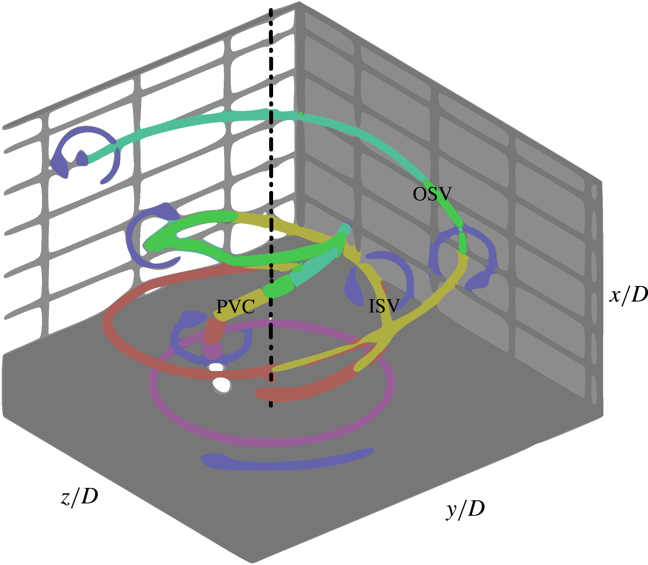
criterion (Jeong & Hussain Reference Jeong and Hussain1995) three precessing spiral vortex structures in a model burner: the PVC, an inner secondary vortex (ISV) and the outer secondary vortex (OSV) (figure 1). In the above study, the PVC is the primary and most powerful structure (characterized by the greatest negative
 $\unicode[STIX]{x1D706}_{2}$
values) as it is associated with the dominant vorticity generated by the swirler; the inner secondary vortex and the outer secondary vortex are considered as secondary since they develop from the instability of the shear layer bounding the high momentum region. The jet breakdown zone is where a pair of co-rotating co-winding helical vortices, the PVC and the inner secondary vortex, meet. Several other works (Oberleithner et al.
Reference Oberleithner, Sieber, Nayeri, Paschereit, Petz, Hege and Wygnanski2011; Markovich et al.
Reference Markovich, Abdurakipov, Chikishev, Dulin and Hanjalić2014) have reconstructed the three-dimensional oscillatory flow pattern from uncorrelated two-dimensional PIV snapshots using proper orthogonal decomposition (POD, Holmes et al.
Reference Holmes, Lumley, Berkooz and Rowley2012) and showed that the flow field is characterized by a single global mode having a dominant frequency corresponding to that of the vortex core precession.
Vortex lines identified from
 $\unicode[STIX]{x1D740}_{2}$
criterion applied on volumetric data of phase-averaged LDA measurements. Illustration adapted from Cala et al. (Reference Cala, Fernandes, Heitor and Shtork2006).

Considering the relevance of swirling jets issued from swirl–vane generators (i.e. a multichannel swirling jet) due to their mechanical simplicity compared to other swirl devices, relatively few works are available in the literature and mostly deal with combustion and heat transfer applications (see e.g. Lilley Reference Lilley1977, or Ianiro & Cardone Reference Ianiro and Cardone2012). The flow field issued from the swirl vanes affects the azimuthal uniformity at the jet exit and introduces an unsteady three-dimensional flow pattern that requires extensive visualization efforts to be understood.
The modelling of swirl flows has been described as ‘a perpetual challenge’ by Jakirlic, Hanjalic & Tropea (Reference Jakirlic, Hanjalic and Tropea2002). More recently Grundmann et al. (Reference Grundmann, Wassermann, Lorenz, Jung and Tropea2012) approached the problem of swirling flows for the case of a swirl tube with a three-dimensional survey of the time-averaged velocity field using magnetic resonance velocimetry (Elkins et al. Reference Elkins, Markl, Pelc and Eaton2003). The complexity of the flow led to the conclusions that more detailed investigations on the topic are needed, especially in relation to the dynamical behaviour of the flow. A further challenge of vane-imparted swirling jets is that the unsteady three-dimensional features exhibited by the non-axisymmetric flow field cannot be fully described with planar measurements. Recent studies have reported that flow events, such as vortex pairing and the vortex core breakdown, do not pertain to a specific plane of symmetry (Ceglia et al. Reference Ceglia, Discetti, Ianiro, Michaelis, Astarita and Cardone2014). Hence, comprehensive studies elucidating the three-dimensional vortex dynamics would require the instantaneous measurement of the velocity and vorticity field in a domain that encompasses the whole jet and the vortex lines, which is possible by tomographic PIV (Elsinga et al. Reference Elsinga, Scarano, Wieneke and van Oudheusden2006).
The measurement of the dynamical behaviour of the swirling jets is relevant to the study of flow stability in relation to combustion and thermo-acoustics (Candel et al. Reference Candel, Durox, Schuller, Bourgouin and Moeck2014). Capturing the frequencies and the global modes dominating the large-scale unsteady behaviour requires measurements at a rate sufficient to resolve the temporal evolution of the flow along with its global organization. The use of high-repetition-rate systems enables time-resolved tomographic PIV (TR-Tomo PIV), which has been used to describe jets without swirl at moderate Reynolds number (Violato & Scarano Reference Violato and Scarano2011; Violato et al. Reference Violato, Ianiro, Cardone and Scarano2012). Moreover the complex unsteady flow organization requires an approach that delivers the swirling jet behaviour in its essence by reducing its number of degrees of freedom. Low-order flow reconstructions have often been attained by means of decomposition into orthogonal modes using POD (see e.g. Oberleithner et al. Reference Oberleithner, Sieber, Nayeri, Paschereit, Petz, Hege and Wygnanski2011), yielding a simplified representation of the dominant flow features. For time-resolved sequences, the synthesis of dynamically significant modes has been demonstrated through the concept of dynamical mode decomposition (DMD, Schmid Reference Schmid2010). The latter allows a linear stability analysis of the flow and modes are sorted on the basis of their growth rate as opposed to POD where the energy content is considered. The suitability of the technique to inspect three-dimensional time-resolved experimental data of a transitional jet has been assessed in the study of Schmid, Violato & Scarano (Reference Schmid, Violato and Scarano2012).
The present work aims at capturing the instantaneous three-dimensional organization and dynamical evolution of swirling jets produced by swirl vanes. The emphasis is put on the instantaneous vortex topology and the relation between the outer shear layer dynamics (Kelvin–Helmholtz vortices, their pairing and global dynamics), and the inner region where the precessing vortex core becomes prominent at higher values of the swirl number. The effect of the jet swirl is investigated conducting several experiments that span the range of swirl number from 0 to 0.8.
Time-resolved tomographic PIV allows us to measure the instantaneous velocity field in a three-dimensional domain from which the full velocity gradient tensor components can be computed. This enables detection of the vortical structures by vortex criteria such as the
 $Q$
-criterion (Hunt, Wray & Moin Reference Hunt, Wray and Moin1988; Jeong & Hussain Reference Jeong and Hussain1995). Furthermore, access to the dynamical evolution of the swirling jet is granted by the time resolution of the measurements, based upon high-speed illumination and imaging hardware for the tomographic PIV system. The approach, adopted to reconstruct the most relevant global modes, follows the sparsity-promoting DMD algorithm (Jovanović, Schmid & Nichols Reference Jovanović, Schmid and Nichols2014) which allows us to select, amongst DMD modes, those which contribute more to the flow field, achieving a trade-off between the quality of the DMD based low-order reconstruction and the number of modes used to approximate the flow fields. The approach returns the spatial pattern of the considered mode along with the associated oscillation main frequency.
In the following sections, the experimental set-up and the measurement procedure are described (§ 2), followed by the discussion of time-averaged flow field properties (§ 3). Further, the analysis of the unsteady flow behaviour and the instantaneous vortex topology is presented (§ 4). Given the three-dimensional complexity of the flow field, the interpretation of the fluid dynamical aspects is supported by three-dimensional visualizations and supplemental digital material with time-resolved animations. Furthermore, the interaction between the vortical structures resulting from the outer shear layers and the central vortex core is discussed by means of a low-order reconstruction of the flow field based on the most relevant dynamical modes (§ 5). This discussion elucidates the relation between shear layer instabilities, vortex core precession and its breakdown for the conditions considered in the present work.
2 Experimental set-up and data reduction
2.1 Experimental set-up
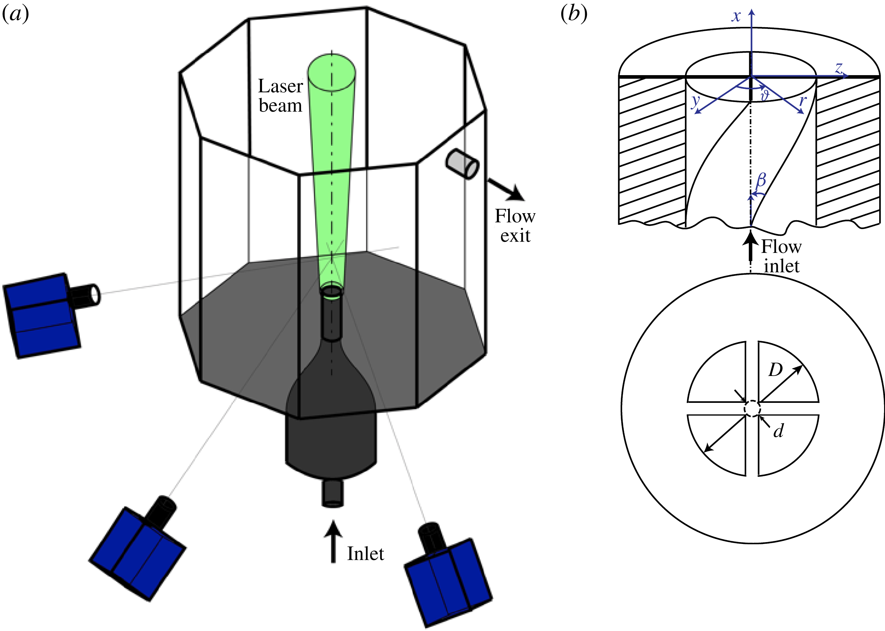
The experiments are performed in the Jet Tomographic Facility at the Aerodynamics Laboratories of TU Delft, an octagonal water tank (600 mm inner diameter and 800 mm height) made of polymethyl methacrylate allowing full optical access for illumination and tomographic imaging. The experimental arrangement follows that described in Violato et al. (Reference Violato, Ianiro, Cardone and Scarano2012). The swirling jet is realized with a nozzle of diameter
 $D=19.7~\text{mm}$
emerging from the bottom wall of the facility (figure 2
a).
Schematic arrangement of the experimental apparatus and set-up: (a) jet tomography facility, with jet nozzle on the bottom and schematic of the tomographic PIV system; (b) detail of swirling nozzle geometry.

Neutrally buoyant polyamide particles with median diameter of
 $56~\unicode[STIX]{x03BC}\text{m}$
(VESTOSINT®2157) are employed as seeding particles. The water circulates in closed circuit to maintain a constant seeding density equal to approximately
 $0.3~\text{particles}~\text{mm}^{-3}$
. The flow rate is controlled through a pump and a valve and monitored by a rotameter (the uncertainty in flow rate measurements is approximately 3 %). The water supply provides a range of stable exit flow rates corresponding to Reynolds numbers
 $Re=4{\dot{m}}/(\unicode[STIX]{x03C0}\unicode[STIX]{x1D707}D)$
between 500 and 15 000. The experiments are performed at
 $Re=1000$
with a bulk axial exit velocity
 $U=0.05~\text{m}~\text{s}^{-1}$
.
The swirling insert consists of a short pipe with a length of approximately 140 mm (
 $7D$
) (figure 2
b) where four vanes impart the swirl to the flow. Immediately after the vanes, the nozzle ends with a sharp exit as a truncated pipe. The vanes are introduced using a cross-helical insert. In this case, the swirl number is related to the swirl vane angle
 $\unicode[STIX]{x1D6FD}$
, the vane pack hub diameter
 $d$
(equal to 1 mm) and the jet nozzle diameter
 $D$
. The definition of the swirl number
 $S$
according to Gupta et al. (Reference Gupta, Lilley and Syred1984) reads as
 $$\begin{eqnarray}\displaystyle S=\frac{2}{3}\left[\frac{1-(d/D)^{3}}{1-(d/D)^{2}}\right]\tan \unicode[STIX]{x1D6FD}. & & \displaystyle\end{eqnarray}$$
The swirl angle of the helical inserts is varied yielding values of
 $S$
spanning the range from 0 to 0.8 in increments of 0.2. The case of a non-swirling jet (
 $S=0$
) is taken for reference since the flow passes through the vanes with no added swirling motion. The weak swirling jet conditions of Liang & Maxworthy (Reference Liang and Maxworthy2005) are represented by the cases
 $S=0.2$
and 0.4, whereas the strong swirling jet conditions are achieved at
 $S=0.6$
and 0.8.
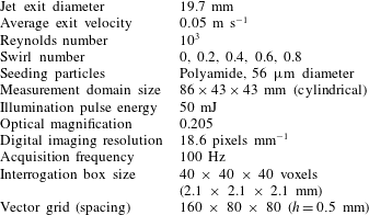
The tomographic PIV set-up is sketched in figure 2(a) and the experimental parameters are summarized in table 1. The illumination for tomographic PIV measurements is provided by a solid-state diode-pumped Quantronix Darwin-Duo Nd-YLF laser (two lasers with an intensity of 25 mJ when operated at 1000 Hz). The laser beam with exit diameter of 6 mm is expanded with a diverging lens to a diameter of 8 cm and then focused with a converging lens towards the nozzle exit, in order to have a quasi-cylindrical illumination volume with a diameter of approximately 50 mm at the top of the measurement domain and 45 mm at the nozzle exit.
Summary of experimental parameters.

The light scattered by the
 $56~\unicode[STIX]{x03BC}\text{m}$
polyamide particles is recorded by a tomographic system composed of three LaVision Imager Pro HS CMOS cameras (2016 pixels
 $\times$
2016 pixels,
 $11~\unicode[STIX]{x03BC}\text{m}$
pixel size) subtending a planar angle of
 $90^{\circ }$
. Nikon objectives of 105 mm focal length are set with a relative aperture
 $f/\#=22$
to allow focused imaging of the illuminated particles over the illuminated domain. For the chosen illumination and imaging configuration the maximum particle image density (approximately 0.04 particles/pixel) is attained on the line of sight intersecting the jet axis and decreases towards the edges of the illumination.
The field of view has a digital resolution of
 $18.6~\text{pixels}~\text{mm}^{-1}$
(pixel image size
 $53.75~\unicode[STIX]{x03BC}\text{m}$
). The jet exit diameter corresponds to 365 pixels. The measurement domain extends for 98 mm along the axial direction and 50 mm in the radial one. Sequences of 200 images of tracer particles are recorded at 100 Hz, providing imaged particle displacements of approximately 10 pixels at the jet exit. The latter conditions enable time-resolved measurements and advanced data analysis based on sequences.
2.2 Tomographic PIV measurement system and procedure
The initial volumetric calibration function obtained with a double-layered dot pattern is corrected by the volume self-calibration technique (Wieneke Reference Wieneke2008) to minimize registration errors. The accuracy of the reconstructed object is improved by reducing background intensity with image pre-processing (sliding minimum subtraction over a neighbourhood kernel of 31
 $\times$
31 pixels). The volumetric light intensity is reconstructed with an advanced technique that combines the multiplicative algebraic reconstruction technique (MART, Herman & Lent Reference Herman and Lent1976) algorithm with the motion tracking enhancement (MTE, Novara, Batenburg & Scarano Reference Novara, Batenburg and Scarano2010) within a sequence-marching approach (SMTE, Lynch & Scarano Reference Lynch and Scarano2015). A unity pixel-to-voxel ratio is applied resulting in a measurement volume of approximately
 $86\times 43\times 43~\text{mm}^{3}$
being discretized with
 $1600\times 800\times 800~\text{ voxels}$
.
The three-dimensional particle motion analysis is performed with the fluid trajectory correlation approach (FTC, Lynch & Scarano Reference Lynch and Scarano2013). A short sequence of 5 objects is used to reproduce the particles pattern motion, which is modelled with a second-order polynomial fit. The interrogation volume size is 40
 $\times$
40
 $\times$
40 voxels (
 $2.1\times 2.1\times 2.1~\text{mm}^{3}$
). The overlap between adjacent interrogation boxes of 75 % leads to a vector pitch of approximately 0.5 mm (
 $0.025D$
). The use of the 200 available snapshots for the present reconstruction and correlation analysis results in a total of 192 available velocity snapshots.
The evaluation of measurement uncertainty is made here on the basis of error estimation coming from imaging, tomographic reconstruction and three-dimensional cross-correlation. Additional uncertainties on the statistical flow properties are due to the finite size of the considered data ensemble.
Tomographic reconstruction of the three-dimensional particle distribution strongly relies upon the precision of the system calibration (Elsinga et al. Reference Elsinga, Scarano, Wieneke and van Oudheusden2006). In the present case, a geometrical calibration yields residual displacements among cameras of the order of 0.3 pixels. The use of the volume self-calibration procedure (Wieneke Reference Wieneke2008) reduces the above disparity to a negligible level 0.03 pixels (corresponding to approximately 1 % of the particle image diameter).
The accuracy of tomographic PIV reconstruction is to date the object of investigation (Lynch & Scarano Reference Lynch and Scarano2014). The effect of ghost particles may lead to a systematic underestimation of the measured particle displacement gradient (Elsinga et al.
Reference Elsinga, Westerweel, Scarano and Novara2011). The intensity of ghost particles is estimated comparing the reconstructed intensity inside the illuminated region and that outside the region of illumination, which defines the reconstruction signal-to-noise ratio
 $\text{SNR}_{R}$
(Lynch & Scarano Reference Lynch and Scarano2014). A value of
 $\text{SNR}_{R}<2$
indicates that the spatial cross-correlation signal is affected significantly by ghost particles, in turn modulating the velocity gradient. In the present case
 $\text{SNR}_{R}>3$
and velocity gradient modulation is expected solely due to the effect of the finite size of the interrogation window. An estimation of uncertainty associated with random errors is made invoking the mass conservation principle. The latter can be used to ascertain the consistency of the measured velocity field as also proposed by Zhang, Tao & Katz (Reference Zhang, Tao and Katz1997). Although the velocity divergence is not commonly considered a property of fluid dynamic interest when dealing with incompressible vortex-dominated flows, its simple formulation makes it a suitable quantity to estimate the measurement errors on the spatial derivatives of the flow (Scarano Reference Scarano2012; Kähler et al.
Reference Kähler, Astarita, Vlachos, Sakakibara, Hain, Discetti, La Foy and Cierpka2016). For incompressible flows the velocity divergence must be zero everywhere and the value of its standard deviation provides a data based estimate for the uncertainty associated with the measurement of the velocity gradient tensor components. In the present measurements, the divergence standard deviation attains typical levels of
 $0.01~\text{voxels}^{-1}$
. Once divided by the typical values observed for the vorticity in the jet shear layer (
 $0.2~\text{voxels}^{-1}$
), the relative uncertainty of the vorticity field is estimated to be of the order of 5 %.
Some local exceptions where the velocity divergence standard deviation is larger than the above indicated value are detected at the edges of the domain, where the tomographic reconstruction is typically poorer, and in the immediate vicinity of the nozzle exit, where the rate of shear is highest. In these regions, the velocity gradient measurement uncertainty can attain 10 %, although these regions are barely considered for the fluid dynamic analysis of the swirling jet. Following the uncertainty analysis of Moffat (Reference Moffat1988) the expected level of uncertainty for the evaluation of the
 $Q$
-criterion is similar to that mentioned for the vorticity. The latter does not affect the process of vortex detection because the chosen values of
 $Q$
are taken at approximately 50 % of the maximum exhibited in the flow domain.
Finally, the uncertainty of the statistical flow properties is evaluated due to the limited number of samples used for the averaging process. Considering that the velocity fluctuations in the jet reach approximately 10 % of the bulk velocity, the uncertainty of the mean velocity from 200 snapshots (correlation coefficient among every two snapshots is 0.5) is estimated to be approximately 2 %. The main limitation to the statistical convergence of the DMD analysis arises from the limited number of shedding and pairing events captured within the experiments. Considering that approximately 10 shedding periods are covered, corresponding to 5 simple pairing and approximately 3 composite pairing periods, the Fourier spectral resolution varies between 10 and 30 % of the characteristic frequencies of these events. The latter makes the mode coefficients analysis somehow qualitative, yet they emerge as local maxima of the DMD eigenvalues.
2.3 Modal decomposition
The dynamic mode decomposition (Schmid Reference Schmid2010; Tu et al. Reference Tu, Rowley, Luchtenburg, Brunton and Kutz2014) extracts dynamic information (the dynamic modes) from a sequence of uniformly sampled flow measurements: these modes are representative of the flow structures which most contribute to the dynamical evolution of the flow along the measured sequence. For the sake of completeness, the main definitions and operations of the DMD procedure are summarized as follows.
A sequence of snapshots is collected in a data matrix whose columns represent the individual data samples. Here a sequence matrix of
 $N+1$
snapshots equally spaced
 $\unicode[STIX]{x0394}t$
in time
 $\{\unicode[STIX]{x1D74D}_{0},\unicode[STIX]{x1D74D}_{1},\ldots ,\unicode[STIX]{x1D74D}_{N}\}$
is considered. From this sequence, two sub-sequences with a unit shift can be obtained:
 $$\begin{eqnarray}\displaystyle \left.\begin{array}{@{}c@{}}\unicode[STIX]{x1D733}_{0}=\{\unicode[STIX]{x1D74D}_{0},\unicode[STIX]{x1D74D}_{1},\ldots ,\unicode[STIX]{x1D74D}_{N-1}\}\\ \unicode[STIX]{x1D733}_{1}=\{\unicode[STIX]{x1D74D}_{1},\unicode[STIX]{x1D74D}_{2},\ldots ,\unicode[STIX]{x1D74D}_{N}\}\end{array}\right\} & & \displaystyle\end{eqnarray}$$
If the system under observation is time-discrete, linear and time-invariant, for
 $t=\{0,1,\ldots ,N\}$
, the evolution of a single snapshot to an adjacent snapshot in time is given by a linear operation
 $\unicode[STIX]{x1D74D}_{t+1}=\unicode[STIX]{x1D63C}\unicode[STIX]{x1D74D}_{t}$
. Due to time-invariance, the latter applies to all snapshots, i.e.
 $\unicode[STIX]{x1D733}_{1}=\unicode[STIX]{x1D63C}\unicode[STIX]{x1D733}_{0}$
. The dynamic mode decomposition is a procedure that yields a low-order representation of the matrix
 $\unicode[STIX]{x1D63C}$
and produces modes which are a tangential linear approximation of the actual nonlinear system matrix.
The modal representation of the DMD algorithm developed by Schmid (Reference Schmid2010) provides a representation
 $\unicode[STIX]{x1D641}$
of the matrix
 $\unicode[STIX]{x1D63C}$
in the basis spanned by the singular vectors of
 $\unicode[STIX]{x1D733}_{0}$
.
The economy-size singular value decomposition of
 $\unicode[STIX]{x1D733}_{0}$
is given by
 $$\begin{eqnarray}\displaystyle \unicode[STIX]{x1D733}_{0}=\unicode[STIX]{x1D650}\unicode[STIX]{x1D72E}\unicode[STIX]{x1D651}^{\ast }, & & \displaystyle\end{eqnarray}$$
where
 $\unicode[STIX]{x1D72E}$
is a diagonal matrix containing the singular values of
 $\unicode[STIX]{x1D733}_{0}$
and the columns of the matrices
 $\unicode[STIX]{x1D650}$
and
 $\unicode[STIX]{x1D651}$
are referred to as the left singular vectors and right singular vectors of
 $\unicode[STIX]{x1D733}_{0}$
, respectively.
The matrix
 $\unicode[STIX]{x1D63C}$
is defined as
 $$\begin{eqnarray}\displaystyle \unicode[STIX]{x1D63C}\approx \unicode[STIX]{x1D650}\unicode[STIX]{x1D641}\unicode[STIX]{x1D650}^{\ast }. & & \displaystyle\end{eqnarray}$$
The matrix
 $\unicode[STIX]{x1D641}$
is determined from the matrices of snapshots
 $\unicode[STIX]{x1D733}_{0}$
and
 $\unicode[STIX]{x1D733}_{1}$
by minimizing the Frobenius norm of the difference between
 $\unicode[STIX]{x1D733}_{1}$
and
 $\unicode[STIX]{x1D63C}\unicode[STIX]{x1D733}_{0}$
defined as in (2.3) and (2.4), i.e.
 $$\begin{eqnarray}\displaystyle \unicode[STIX]{x1D641}_{DMD}=\unicode[STIX]{x1D650}^{\ast }\unicode[STIX]{x1D733}_{1}\unicode[STIX]{x1D651}\unicode[STIX]{x1D72E}^{-1}. & & \displaystyle\end{eqnarray}$$
The modal structures are extracted from the matrix
 $\unicode[STIX]{x1D641}_{DMD}$
by multiplying
 $\unicode[STIX]{x1D650}$
times the matrix containing the right eigenvectors
 $\unicode[STIX]{x1D654}_{DMD}$
of
 $\unicode[STIX]{x1D641}_{DMD}$
:
 $$\begin{eqnarray}\displaystyle \unicode[STIX]{x1D731}=\unicode[STIX]{x1D650}\unicode[STIX]{x1D654}_{DMD}. & & \displaystyle\end{eqnarray}$$
The snapshot sequence can now be written as
 $$\begin{eqnarray}\displaystyle \unicode[STIX]{x1D733}(t)=\mathop{\sum }_{n=1}^{N-1}\unicode[STIX]{x1D6FC}_{n}\unicode[STIX]{x1D753}_{n}\unicode[STIX]{x1D707}_{n}^{t}, & & \displaystyle\end{eqnarray}$$
where
 $\unicode[STIX]{x1D707}_{n}$
is the
 $n$
th complex eigenvalue of
 $\unicode[STIX]{x1D641}_{DMD}$
and
 $\unicode[STIX]{x1D6FC}_{n}$
is the ‘amplitude’ of the
 $n$
th DMD mode. The eigenvalue
 $\unicode[STIX]{x1D707}_{n}$
contains information about the underlying temporal frequencies and growth/decay rates of the
 $n$
th DMD mode: the real and the imaginary parts of
 $\unicode[STIX]{x1D706}_{n}=\log (\unicode[STIX]{x1D707}_{n})/\unicode[STIX]{x0394}t$
represent the damping/growth rate and the frequency of the mode, respectively. The frequency of the dynamic modes is reported in the following in the form of the Strouhal number
 $St=\text{Im}(\unicode[STIX]{x1D706}_{n})D/2\unicode[STIX]{x03C0}U$
.
The computation of the values of the coefficients
 $\unicode[STIX]{x1D6FC}_{n}$
is described by Jovanović et al. (Reference Jovanović, Schmid and Nichols2014), who also show that the choice of the most significant modes for a low-order reconstruction is non-trivial. This is due to the possibility that the largest amplitude fluctuations originate from strongly damped eigenvalues. The above authors have proposed therefore a method to promote sparsity (i.e. to have several values of
 $\unicode[STIX]{x1D6FC}_{n}=0$
) by selecting only the most significant modes. The resulting method is used herein to extract the most relevant modes of the vortex dynamics under investigation.
3 Time-averaged flow field
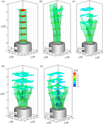
A summary of the time-averaged flow field for varying swirling strength is illustrated in figure 3: the jets are visualized with isosurfaces of streamwise velocity
 $\bar{u}/U=0.5$
, highlighting approximately the mean shear layer and
 $\bar{u}/U=-0.1$
, which gives an indication of the reverse flow region. Cross-sections describing the axial velocity contours are selected at several stations between
 $x/D=0.1$
and
 $x/D=4$
.
Time-averaged velocity distribution of the jets with varying swirl numbers. Isosurfaces at
 $\overline{u}/U$
equal to 0.5 and
 $-0.1$
. Cross-stream slices with contours of
 $\overline{u}/U$
.

As opposed to the works where the swirl is imparted by a rotating tube at the exit (Billant et al. Reference Billant, Chomaz and Huerre1998; Örlü & Alfredsson Reference Örlü and Alfredsson2008), in this work the four vanes generate a non-homogeneous velocity distribution along the azimuthal direction from the very exit of the jet. The resulting flow features a jet divided into four sectors separated by the wakes produced by the boundary layer developed along the vane walls. After the exit, the internal wake develops with a rapid homogenization of momentum inside the jet. On the external boundary, the jets interact with the surrounding quiescent fluid through a shear layer that follows approximately a four-lobed contour.
At
 $S=0$
(figure 3
a) the axial velocity exhibits four maxima in the centre of each of the four sectors and the velocity profile is close to a parabolic distribution; each of the four jets behaves as a laminar jet issuing from a pipe and they are separated by the thin wake of the insert. The separation between the four jets vanishes after approximately four diameters from the exit.
As the swirl is introduced (figure 3
b–e), the location of the maximum axial velocity is displaced outwards and the velocity distribution departs from the parabolic shape with the maximum of velocity moving downstream with respect to the swirl motion in the
 $y$
–
 $z$
plane.
The development of the inner wakes and of the outer shear layers is also influenced by the swirl number. With no swirl (figure 3
a) the multichannel jet exhibits a very slow broadening due to the absence of shear layer instabilities, as discussed later. In contrast, the experiments return already from
 $S=0.2$
a significant spatial separation between the adjacent jet sectors. Moreover, the noticeable increase in their cross-section anticipates the presence of large-scale instabilities occurring in the lobed shear layer. Park & Shin (Reference Park and Shin1993) reported that the effect of swirl on the spreading angle of the jet is quite noticeable and that the swirl has a substantial influence on the entrainment rate. The swirling motion (figure 3
b–e) is found to enhance the broadening of the jet evolving downstream; at the same time, the outer shear layer comes into contact with the inner wakes and in the
 $y$
–
 $z$
cross-section the swirling jets have a shape resembling a Japanese shuriken (see also figure 10). At a distance of
 $1.5D$
from the exit, the jet width (identified with the isosurface of
 $\bar{u}/U=0.5$
) increases with increasing swirl number. At the same time the maximum axial velocity is significantly lower due to momentum conservation. When the swirl number is sufficiently high (
 $S>0.6$
, figure 3
d–e), a recirculation zone develops on the jet axis as visualized by the isosurfaces of
 $\bar{u}/U=-0.1$
in blue. This is found at
 $x/D\approx 1.2$
in the case with
 $S=0.6$
; the recirculation region moves closer to the nozzle exit, in the jet at
 $S=0.8$
.
3.1 A posteriori evaluation of swirling strength
It is interesting to note that, while the swirling nozzles are designed according to the equation for swirling jets with swirl vanes (2.1) as derived by Gupta et al. (Reference Gupta, Lilley and Syred1984), this value differs slightly from the actual swirl number measured from velocity data as in (1.1) (as done e.g. in Oberleithner et al. Reference Oberleithner, Sieber, Nayeri, Paschereit, Petz, Hege and Wygnanski2011).
According to the conservation of momentum in a submerged jet (Rajaratnam Reference Rajaratnam1976), the swirl number is independent of the axial location at which it is measured. The measured swirl number
 $S_{m}$
is thus evaluated downstream of the nozzle exit (at
 $x/D=0.5$
) in order to avoid errors due to laser reflections on the nozzle exit. Equation (2.1) is found to overestimate
 $S$
with an error decreasing with increasing swirl number since values of measured swirl number
 $S_{m}=\{0,0.13,0.31,0.54,0.76\}$
are measured for design swirl numbers
 $S$
equal to
 $\{0,0.2,0.4,0.6,0.8\}$
. This behaviour may be explained by the overshoot of axial velocity at a radial position significantly away
 $(0.35D)$
from the jet axis since in the denominator in (1.1) the square of the axial velocity is weighted with the radial distance.
Despite the above discrepancy, the jet with
 $S=0.6$
(corresponding to
 $S_{m}=0.54$
) retains the peculiarity of the vortex breakdown with central recirculation zone as expected for high swirl jets. Already Vanierschot & Van den Bulck (Reference Vanierschot and Van den Bulck2008) have shown that the centre of the insert may act as a bluff body, inducing a central recirculation even without swirl (as typically widespread in bluff body stabilized flames: see e.g. Shanbhogue, Husain & Lieuwen Reference Shanbhogue, Husain and Lieuwen2009). As it will be shown later, the presence of the central recirculation zone here appears to be promoted by the vortical features developed in the outer shear layer and penetrating through the central thin wake of the insert.
4 Instantaneous flow organization
The velocity field and the associated vortex topology follow the organization of the jets with four sectors. The flow features a principal shear layer dominated by azimuthal vorticity and an inner shear layer associated with the four sectors, with vorticity aligned along the radial direction. Varying the swirling strength, in agreement with the results by Liang & Maxworthy (Reference Liang and Maxworthy2005), three different regimes are identified and discussed: the case with no swirl, that with finite swirl but without vortex breakdown (
 $S=0.2$
and 0.4) and the regimes with vortex breakdown and reverse flow (
 $S=0.6$
and 0.8). The spatio-temporal evolution of the flow is further illustrated with animations for the cases at
 $S=0.2$
, 0.4 and 0.6 provided as supplementary material (movies 1, 2 and 3) available at https://doi.org/10.1017/jfm.2018.140.
4.1 Multichannel jet with no swirl
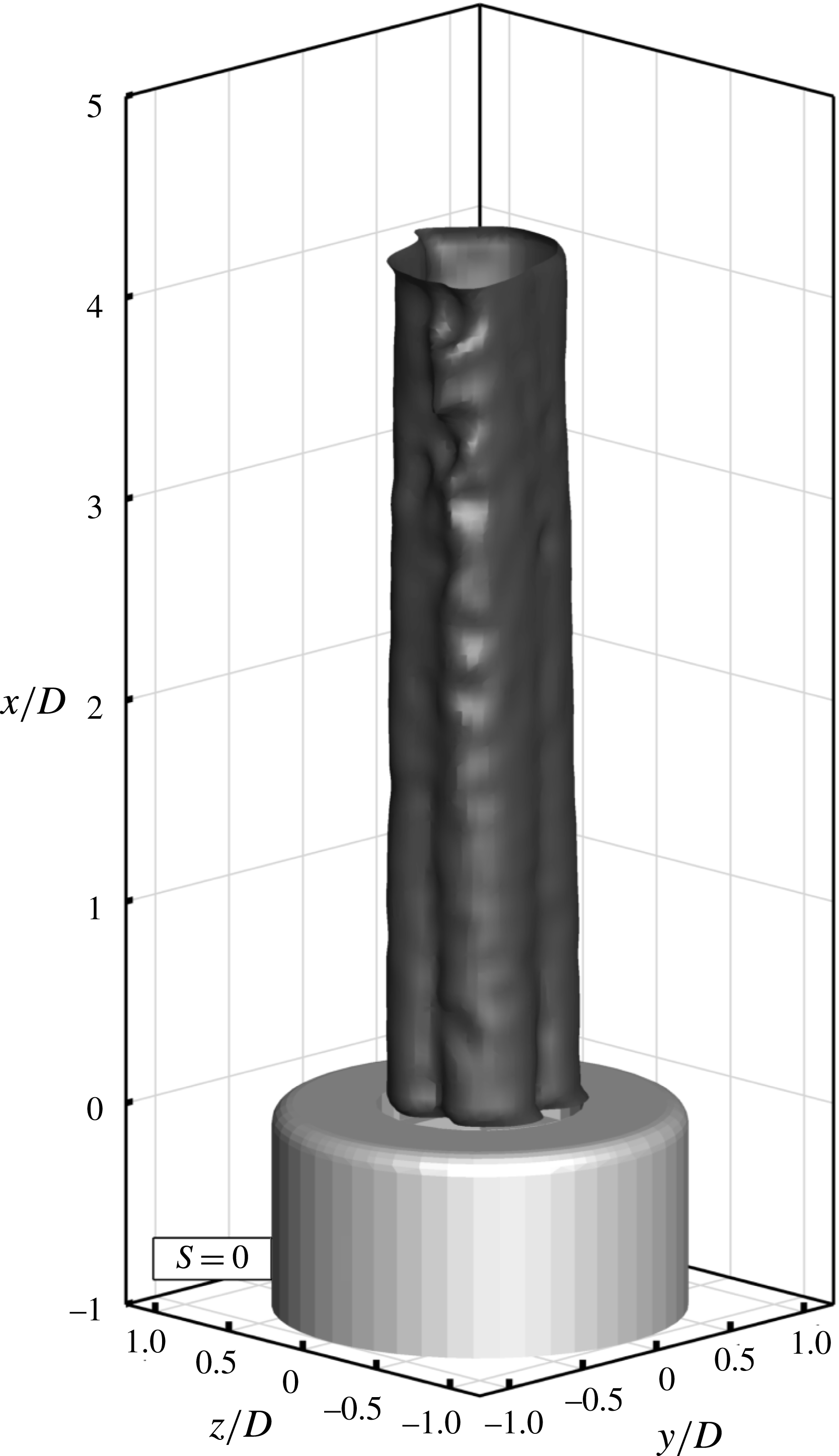
In the absence of swirl, interestingly, no growth of shear layer instabilities is observed. This is in contrast with results obtained for circular jets issued from a sharp-edged orifice at similar Reynolds number (e.g. Beavers & Wilson Reference Beavers and Wilson1970). From the observation of figure 4 it is clear that the jet has a very slow spreading rate, and the shear layer appears only weakly deformed at a distance of three diameters downstream of the nozzle. This indicates an apparent development in the laminar regime.
 $S=0$
, instantaneous flow field: isosurface of
 $u/U=0.7$
.

The absence of Kelvin–Helmholtz vortices is ascribed to the velocity profile at the jet exit, featuring a quasi-parabolic distribution corresponding to the moderate Reynolds number investigated. The shear rate of the jet issued by a sharp orifice studied by Beavers & Wilson (Reference Beavers and Wilson1970) is presumably higher due to the absence of a development length for the boundary layer prior to its detachment at the exit. The above authors reported an earlier formation of Kelvin–Helmholtz vortices. This could be justified by the shear layer being more prone to the onset of instabilities due to the higher shear level, but also because of the phenomenon of vena contracta (Torricelli Reference Torricelli1643) that also introduces streamline curvature at the exit. Furthermore, in the present experiments the interaction between the internal wake and the outer shear layer may act as an additional factor inhibiting formation and roll-up of ring vortices.
4.2 Swirling jets without vortex breakdown
At
 $S=0.2$
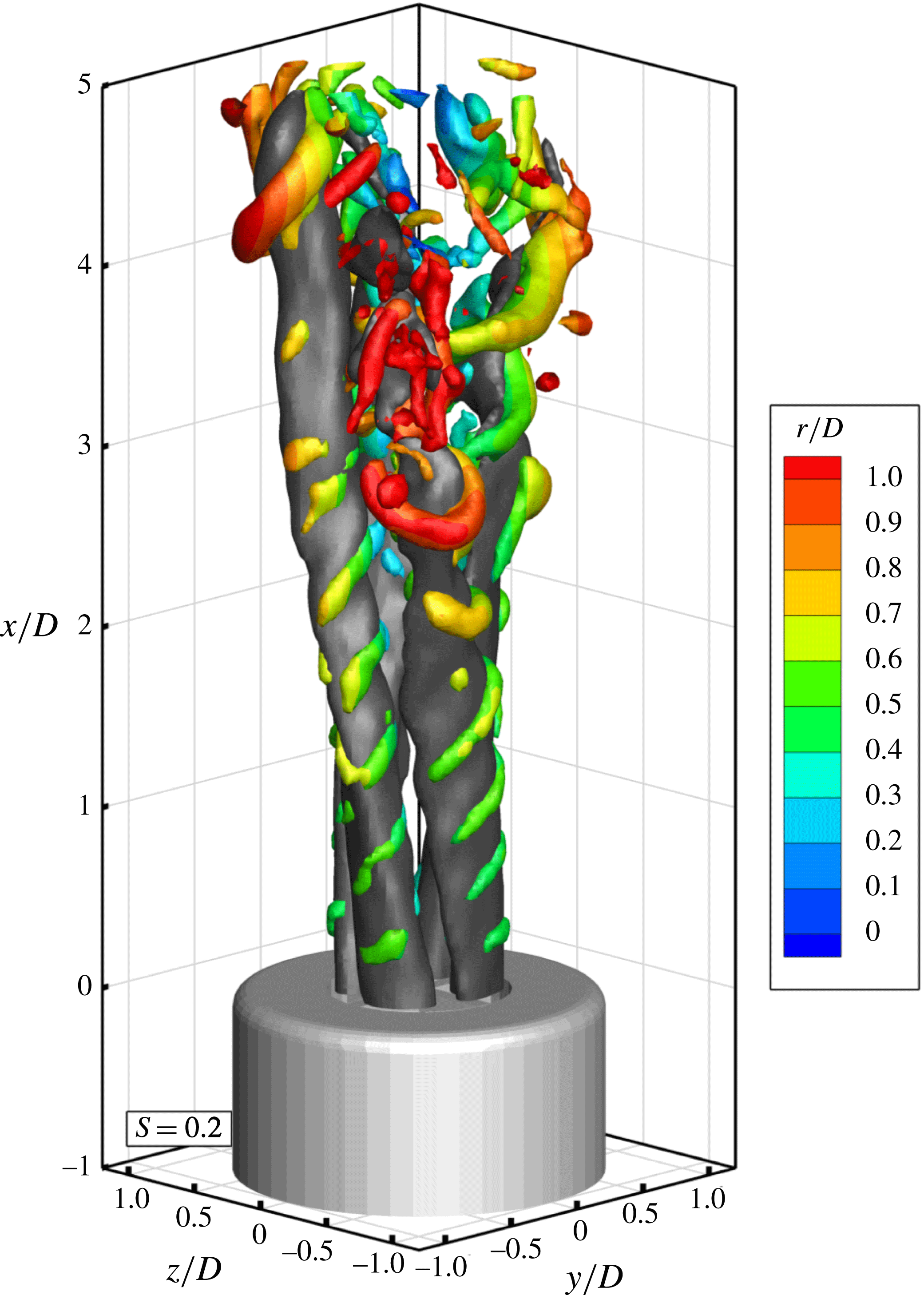
the main coherent structures have the shape of helices that surround the outer part of each jet section (figure 5 and movie 1), each sector having its own helix. The helix advances axially, rotating in the direction opposite to that of the swirl. The pitch of the helix is approximately
 $1.1D$
. However the spacing between two subsequent vortices is approximately
 $0.55D$
, which indicates a double helix arrangement of vortices that wraps each jet sector. Helical structures at a similar swirl number have been previously described for swirling jets issued by a circular nozzle by Liang & Maxworthy (Reference Liang and Maxworthy2005). As visualized in figure 5, the helical vortices take their inception directly after the nozzle exit near to the location of the maximum of axial velocity as illustrated in figure 5, and surround the external shear layer of the jet. In the first part of the jet, the helix is not visible in the interior region. As the jet evolves downstream, these vortical features seem to penetrate also towards the centre of the jet.
Instantaneous flow field at
 $S=0.2$
. Overall jet organization, axial velocity isosurface at
 $u/U=0.7$
in dark grey,
 $Q$
-criterion vortices visualization with isosurfaces of positive
 $Q$
colour-coded with radial distance from the jet axis.

Vortex pairing is observed to occur near
 $x/D=3$
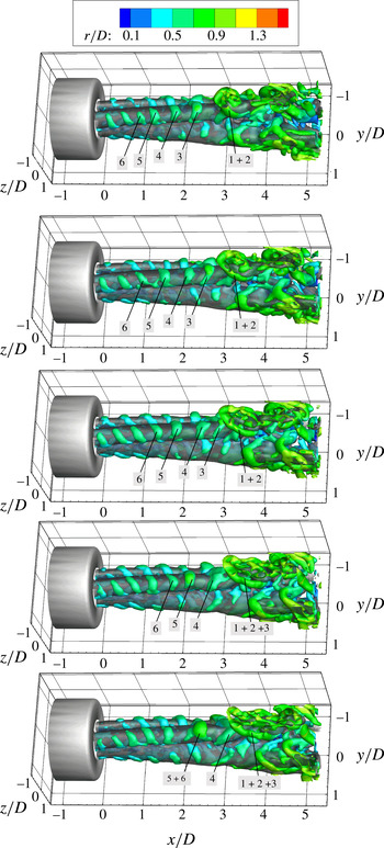
. The resulting structure emerging after pairing exhibits not only a stronger circulation but also an increased azimuthal coherence. As shown in movie 1, vortices pair simultaneously in the external and in the internal part of the jet shear layer through a non-regular process, often involving three vortices. An annotated image sequence is reported in figure 6; snapshots are separated by half convection time
 $D/U$
. The sequence illustrates vortices from the outer shear layer (
 $1+2$
), which undergo pairing, followed by another vortex (3) which is being accelerated towards the centre of the jet and later participates in the pairing process. The structure formed by vortices
 $1+2$
is stretched and elongated toward the outer part of the jet resulting in a significant decrease of its convection velocity while vortex 3 is accelerated. Further upstream, vortex 4 remains isolated, whereas vortices 5 and 6 pair interact similarly to 1 and 2. Before pairing, the following helical vortex undergoes pronounced tilting with the most exterior (interior) portion of the vortex being lifted upwards more rapidly than the interior (exterior) one. The subsequent paired vortices feature a horseshoe shape with the head region retarded (lifted) with respect to the legs. Further away from the exit, the topology of vortex filaments becomes more complex and irregular. Nevertheless, in movie 1 numerous horseshoe vortices can be observed with a periodic behaviour in the space between individual sectors.
Annotated image sequence with temporal separation equal to
 $0.5D/U$
. Axial velocity isosurfaces at
 $u/U=0.7$
in dark grey, isosurfaces of positive
 $Q$
colour-coded with radial distance from the jet axis.

Increasing the swirl number to
 $S=0.4$
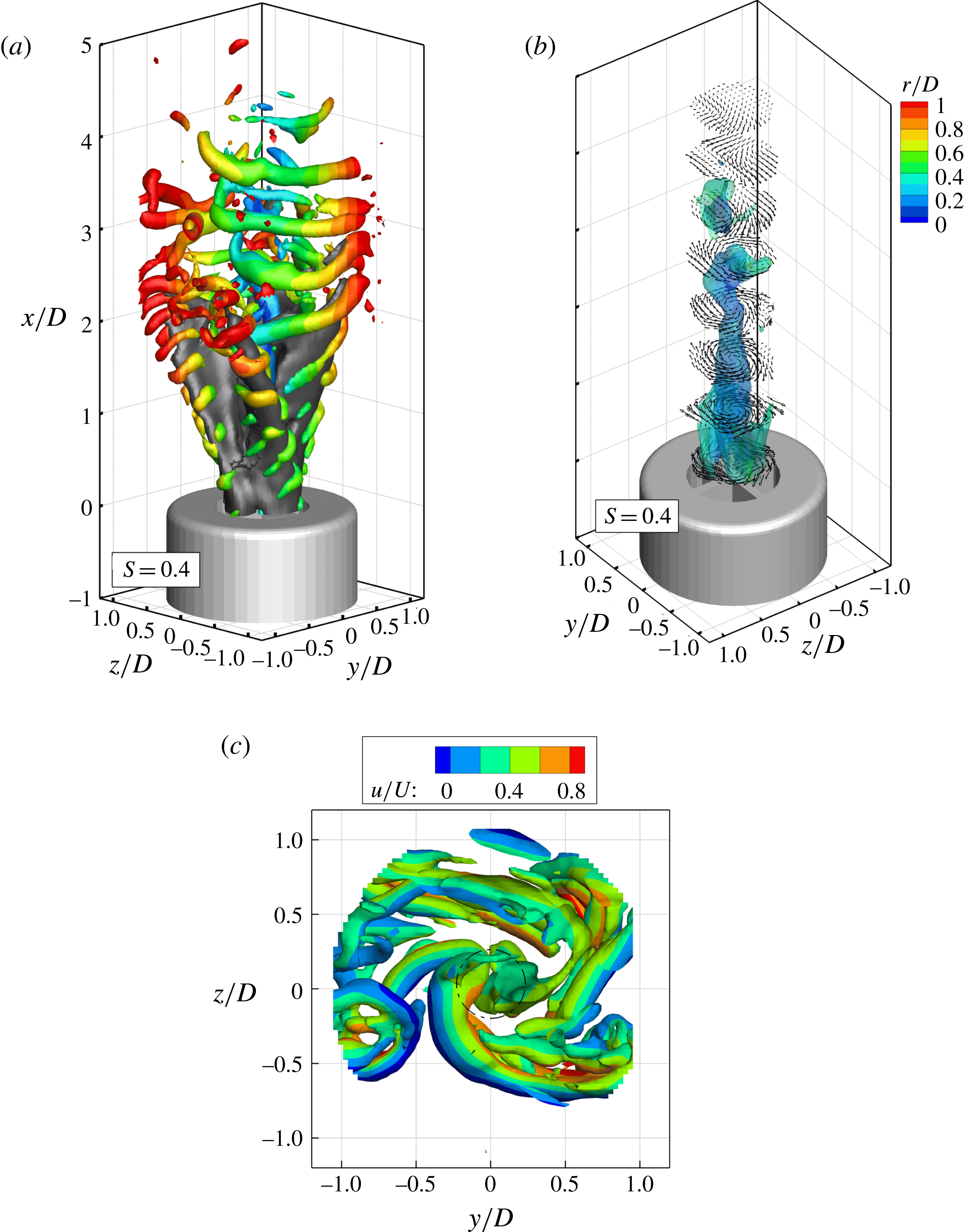
, the vortices formed at the outer edge of the jet sectors undergo earlier pairing approximately two diameters downstream of the nozzle exit. The process results in vigorous rib-like vortices (figure 7
a) which also interconnect among the adjacent sectors and assume a shuriken shape, as shown in figure 7(a,c). Differently from the case at
 $S=0.2$
, the vortex structures do not appear to break down in the higher region of the jet. Instead, the flow pattern becomes dominated by the periodic shedding of rib vortices.
Instantaneous flow organization at
 $S=0.4$
. (a) Axial velocity and vortex topology. Isosurfaces and colouring identical to figure 4. (b) View of vortex core at
 $r/D<0.5$
with isosurface of axial vorticity and vectors projected along the
 $y$
–
 $z$
plane. (c) Top view of instantaneous vortex organization at
 $S=0.4$
. Vortex core indicated by dashed circle.

The central vortex core exhibits a columnar structure for the first two diameters after the exit. The interaction with the shuriken vortices produces a helical shape of the columnar vortex in the upper region of the jet (figure 7 b), which is identified as the precessing vortex core (PVC). The latter phenomenon appears as a precursor to the vortex breakdown, as recently observed at a similar swirl number by Markovich et al. (Reference Markovich, Abdurakipov, Chikishev, Dulin and Hanjalić2014). While the vortex core appears to be too weak to induce reverse flow along the jet axis, a low-speed region is identified near to the axis of the jet in correspondence with the streamwise coordinate where the central vortex core assumes a helical shape. At approximately three diameters from the exit, the PVC loses coherence. Although this could be associated with the conservation of angular momentum with the increase of cross-section (negative vortex stretching), this sudden disappearance of the PVC is instead ascribed to the interaction with the vigorous rib vortices as illustrated in figure 7(c) and further detailed in the data animation (movie 2).
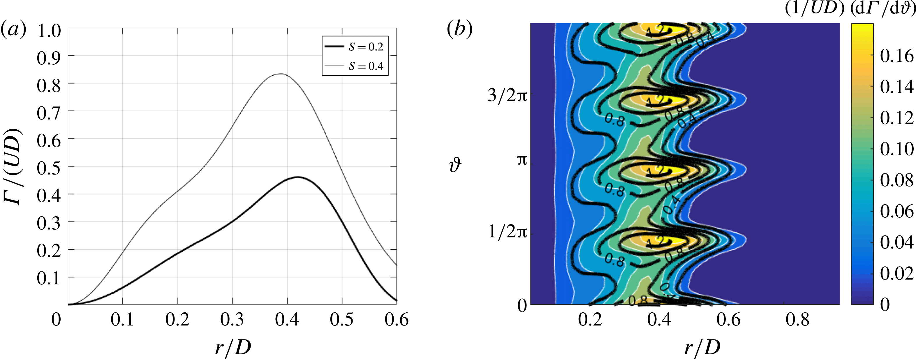
The formation and growth of the helical vortices in the jet shear layer have to be ascribed to the presence of swirl, which has a destabilizing effect on the axial shear layer, since when the azimuthal velocity decreases abruptly outside the core of the vortex, the drop in circulation is known to induce centrifugal and azimuthal Kelvin–Helmholtz instabilities (Gallaire & Chomaz Reference Gallaire and Chomaz2003). Varying the radial distance
 $r$
from the jet axis, the circulation
 $\unicode[STIX]{x1D6E4}$
over closed circles is evaluated on the time-averaged flow fields and reported in figure 8(a) for
 $S=0.2$
And
 $S=0.4$
. The maximum of circulation is found at approximately 0.4 diameters from the jet axis and the helical vortices surrounding the jet are expected to appear at this radial location, as found in previous works on swirling jets (e.g. Billant et al.
Reference Billant, Chomaz and Huerre1998 or Liang & Maxworthy Reference Liang and Maxworthy2005).
Circulation measured in the plane at
 $x/D=0.1$
(a) Mean circulation versus radial coordinate
 $r$
. (b) Colour contours of local circulation
 $\text{d}\unicode[STIX]{x1D6E4}/\text{d}\unicode[STIX]{x1D717}$
and contour lines (in black) of axial velocity in the
 $r$
–
 $\unicode[STIX]{x1D717}$
plane.

It is interesting to inspect the variation along the azimuthal coordinate
 $\unicode[STIX]{x1D717}$
of the local contribution to circulation
 $\text{d}\unicode[STIX]{x1D6E4}/\text{d}\unicode[STIX]{x1D717}=\bar{u}_{\unicode[STIX]{x1D717}}r$
; this gives a better insight than the simple circulation since it allows us to account for the effect of the non-homogeneous velocity distribution along the azimuthal direction. A contour plot of
 $\text{d}\unicode[STIX]{x1D6E4}/\text{d}\unicode[STIX]{x1D717}$
along with the axial velocity (contour lines) is reported in figure 8(b) for the case at
 $S=0.4$
. Both the maximum of axial velocity and that of
 $\text{d}\unicode[STIX]{x1D6E4}/\text{d}\unicode[STIX]{x1D717}$
are located at the same azimuthal location, while the maximum of
 $\text{d}\unicode[STIX]{x1D6E4}/\text{d}\unicode[STIX]{x1D717}$
is found at an outer radial position rather than the maximum of
 $\overline{u}$
. This justifies the formation of helical vortices, especially in the outer parts of the jets corresponding to the azimuthal coordinate of the axial velocity maximum, where both the drop of
 $\text{d}\unicode[STIX]{x1D6E4}/\text{d}\unicode[STIX]{x1D717}$
and the gradient of axial velocity across the shear layer are higher.
4.3 Swirling jets with vortex breakdown
A further increase of
 $S$
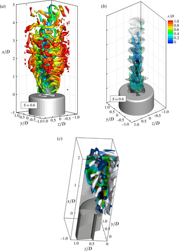
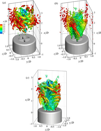
from 0.4 to 0.6 corresponds to a stronger broadening of the jet; as such, helical vortices (which are expected to be shed at a similar Strouhal number as for the other swirl cases, thus having a similar streamwise pitch around the jet inserts) appear as rib-like structures visible on the outer side of the jet sectors (figure 9
a), which connect to weaker vortices on the inner side of the jet. Further upwards, the vortices establish in the azimuthal direction. The rib vortices do not appear to undergo regular pairing, although the interaction occasionally leads to larger and more coherent vortices in the upper region of the jet formed at a distance from the nozzle exit shorter than in the case at
 $S=0.4$
.
Instantaneous flow organization at
 $S=0.6$
. (a) Axial velocity and vortex topology; isosurfaces and colouring identical to figure 4. (b) View of vortex core at
 $r/D<0.5$
with isosurface of axial vorticity and vectors projected along the
 $y$
–
 $z$
axis. The black surface indicates a region of reverse flow at
 $u=-0.1U$
. (c) Magnified view of the interaction between the vortex core and rib vortices, vortex visualization with
 $Q$
criterion colour coded with the sign of the azimuthal vorticity component and vector arrows at plane
 $y/D=-0.1$
.

A surrogate of vortex pairing is also observed at
 $S=0.6$
as a result of the interaction between the rib-like vortices emanating from the jets of each sector as visible in movie 3. The onset of larger vortices with extended azimuthal coherence is observed starting at approximately three diameters from the jet exit. It is possible to argue that, differently with respect to Panda & McLaughlin (Reference Panda and McLaughlin1994), the swirling motion does not suppress the pairing. Indeed, the pairing should be promoted by the swirling motion. The jet broadening due to the swirl, for the conservation of axial momentum, must result in the deceleration of the jet flow as it moves downstream. As a consequence, the preceding vortex is significantly slower than the following one. Based on this consideration the vortex pairing should occur at a further upstream location as the swirl number is increased. This result is in agreement with the work by Liang & Maxworthy (Reference Liang and Maxworthy2005) where the vortex pairing, even if not discussed in the text, is clearly visible for
 $S=1.03$
.
The central vortex core is illustrated in figure 9(b). As assessed in Leibovich (Reference Leibovich1984), an increase in the vane angle results in an increase of the vortex core diameter with respect to the case at
 $S=0.4$
. The vortex features an overall axial pattern and is later formed by a double helical structure. The columnar vortex core, at a distance of approximately 1.2 diameters from the nozzle (figure 9
a) breaks in a double helix (figure 9
b) in agreement with Sarpkaya (Reference Sarpkaya1971). This vortex core breakdown results in a quasi-axisymmetric bubble of recirculating fluid. These patterns could be argued to be due to the presence of the time-averaged recirculation region on the jet axis, visualized in figure 3. It is interesting to note that the vortex breakdown is triggered at an effective swirl number lower than the classical critical number of 0.6 (the measured value of the swirl number
 $S_{m}=0.54$
). The PVC appears to be dominated by helical vortex filaments fed by the vorticity of the vortices which develop in the outer shear layers of the jet and penetrate towards the jet centre (figure 9
c). Brown & Lopez (Reference Brown and Lopez1990) proposed a physical mechanism for vortex breakdown which relies on the production of a negative azimuthal component of vorticity. Later Kurosaka et al. (Reference Kurosaka, Cain, Srigrarom, Wimer, Dabiri, Johnson, Hatcher, Thompson, Kikuchi, Hirano, Yugé and Honda2006) stated that an even weaker condition is needed to promote the vortex breakdown, i.e. just a negative gradient of azimuthal vorticity. The production of azimuthal vorticity, in the case considered by Brown and Lopez (i.e. confined flow and swirling pipe flow), is due to the tilting of streamwise vorticity (
 $\unicode[STIX]{x1D714}_{x}$
) into negative tangential vorticity (
 $\unicode[STIX]{x1D714}_{\unicode[STIX]{x1D717}}$
); instead, in this experiment, as shown in figure 9(c), the azimuthal vorticity is generated in the outer shear layer (rib/shuriken vortices) and penetrates towards the centre of the jet (i.e. towards the vortex core) through the meanders of the jet cross-section. This mechanism is elucidated in figure 9(c), where the induced flow field of the rib vortex (after the pairing between Kelvin–Helmholtz vortices) convectively tilts the vortex core, promoting the vortex breakdown and the formation of the double precessing helix.
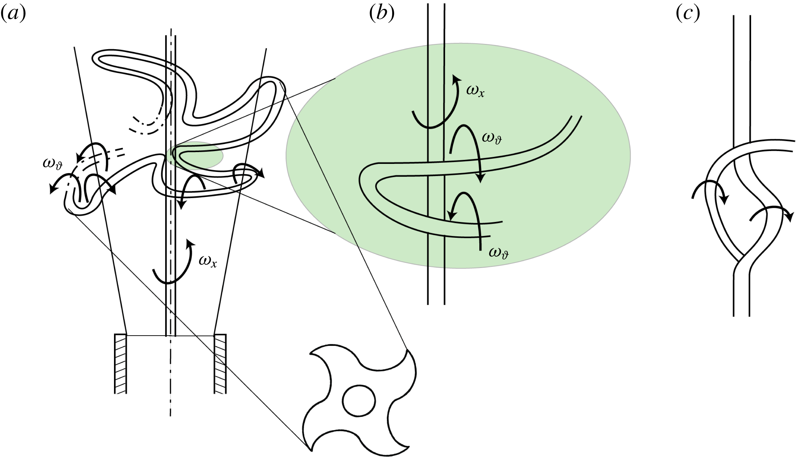
A simplified schematic description is delivered in figure 10 illustrating the outer helical vortex penetrating towards the inner region through the meanders of the vane insert (figure 10
a). The shuriken shape introduces a sign reversal of the azimuthal vorticity since the same vortex is tilted in the proximity of the central vortex core (figure 10
b). At this point the helical vortex interacts with the vortex core; this interaction is especially strong because the two vortices have similar size (Davidson Reference Davidson2015). Vortex tilting and stretching (which can be expressed as
 $\unicode[STIX]{x1D74E}\boldsymbol{\cdot }\unicode[STIX]{x1D735}\unicode[STIX]{x1D651}$
) produce a final result as in figure 10(c) in which the lower part of the helical azimuthal vortex is dissipated due to the strong strain rate in proximity to the central vortex core.
At
 $S=0.8$
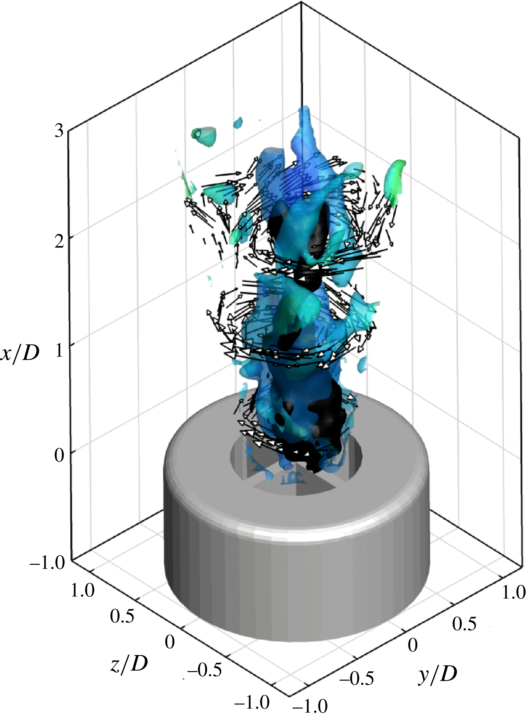
, due to the increase in the swirl number, the phenomenon of vortex breakdown is triggered immediately at the exit as shown in figure 11. Two helical vortices surround the recirculation region that loses axial symmetry. These vortices are located near to the jet axis and extend up to a distance of about 2.5 diameters downstream of the exit.
Schematic of the mutual interaction between azimuthal and axial vorticity leading to vortex breakdown.

 $S=0.8$
, instantaneous flow field: visualization of the spiral helices in translucent blue surrounding the recirculation region in black and velocity vectors in selected
 $x$
planes.

5 Representation by dynamic modes
5.1 Vortex formation and pairing at low swirl
The formation of vortex ring structures in the near region of circular jets is well known from several studies conducted over a wide range of Reynolds number (see e.g. Yule Reference Yule1978). In the present experiments on swirling jets, the shedding of rib-like helical vortices is observed to occur immediately at the nozzle exit as shown in figure 5. The dynamic mode decomposition analysis of the flow near the nozzle exit (
 $x/D<1.6$
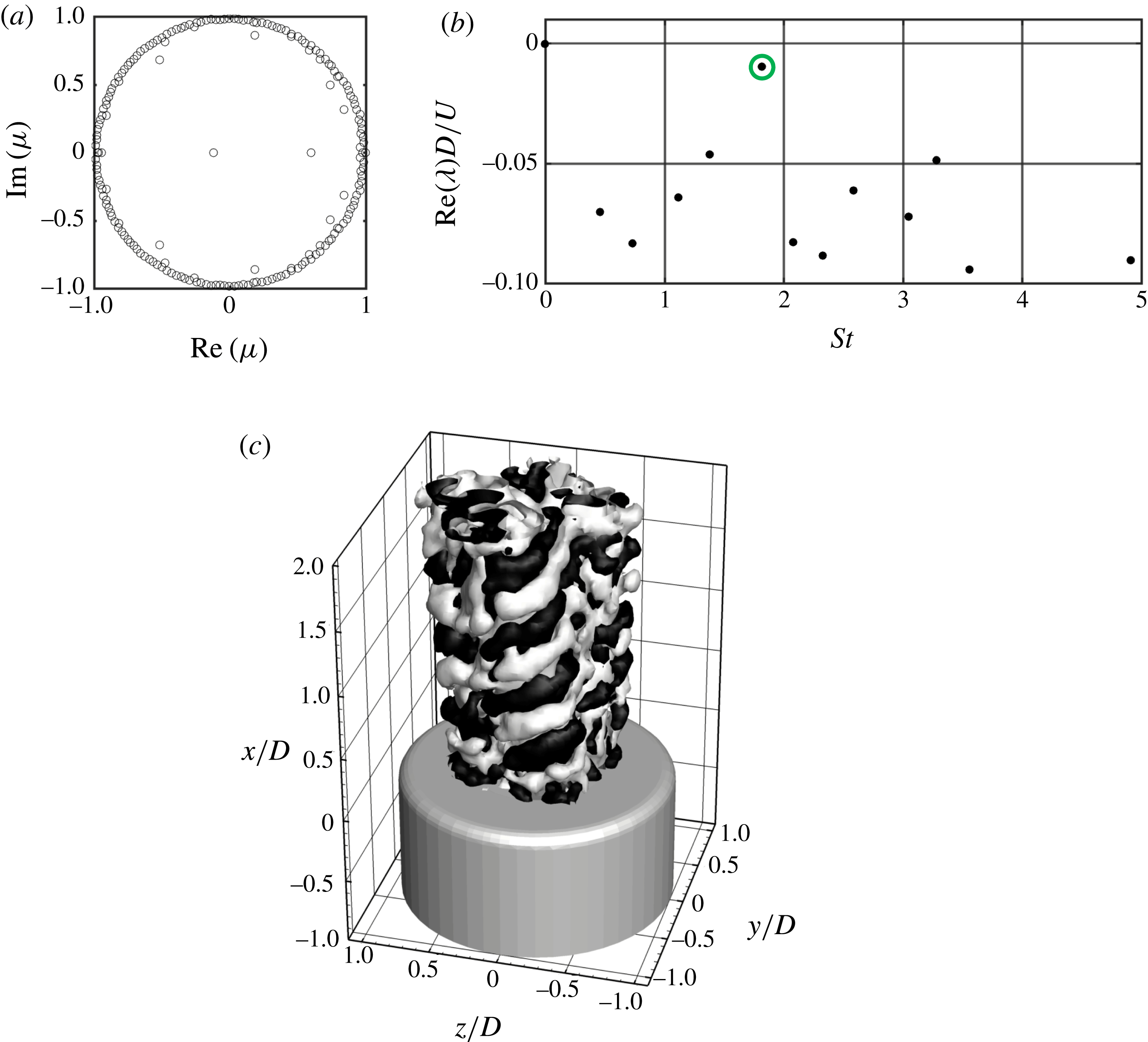
) yields the statistically relevant events in terms of eigenvalues and velocity fluctuations associated with the fastest growing modes. The clustering of the eigenvalues on the unit disk indicates the statistical convergence towards a linear representation of the saturated nonlinear process (Schmid et al.
Reference Schmid, Violato and Scarano2012) as shown in figure 12(a). The mode growth rate is represented versus the corresponding Strouhal number
 $St$
(figure 12
b). Modes with the least damping are considered dominant in that they are associated with the events that decay the least rapidly. The identification of such modes is improved using a sparsity maximization algorithm (Jovanović et al.
Reference Jovanović, Schmid and Nichols2014). In the near exit region, the dominant mode corresponds to
 $St=1.75$
(highlighted with a circle in figure 12) while the (non-dimensionalized) real part of
 $\unicode[STIX]{x1D706}$
is equal to
 $-0.01$
(see figure 12
b).
Dynamic mode decomposition in the near jet exit region at
 $S=0.2$
. (a) Polar plot of complex eigenvalues. (b) Normalized frequency spectrum of dynamic mode damping (the negative part of the spectrum is omitted for brevity). (c) Real part of mode amplitude for
 $St=1.75$
(check value), yielding the helical structure of the outer shear layer. Representation by isosurfaces of positive (white) and negative (black) velocity fluctuations.

The spatial distribution of this mode is visualized with isosurfaces of positive (white) and negative (black) axial velocity fluctuations (figure 12
c). This mode represents the shedding of vortices in the outer shear layer, which are tilted with respect to the
 $x$
–
 $z$
plane and are organized, forming helices; although not evident in figure 5. Figure 12(c) shows that the helical vortices, which develop around the four sectors, have a strong phase correlation as they appear statistically locked onto each other. The situation is observed unambiguously with a tilting view provided in movie 1. The vortex spacing is approximately
 $0.55D$
, with a behaviour similar to the ring vortices developing at the boundary of circular jets, which undergo pairing in the range between 2.5 and 3.5 diameters from their inception point.
The pairing mechanism of ring vortices in circular jets is well assessed (see e.g. Winant & Browand Reference Winant and Browand1974). The phenomenon is also known as leapfrogging (Riley & Stevens Reference Riley and Stevens1993), whereby the flow induced by the preceding vortex produces radial contraction and axial acceleration of the following vortex. The latter is attracted closer to the preceding vortex with the pair undergoing a precession motion. The pairing often leads to rapid growth of azimuthal instabilities involving vortex tilting and stretching followed by breakdown.
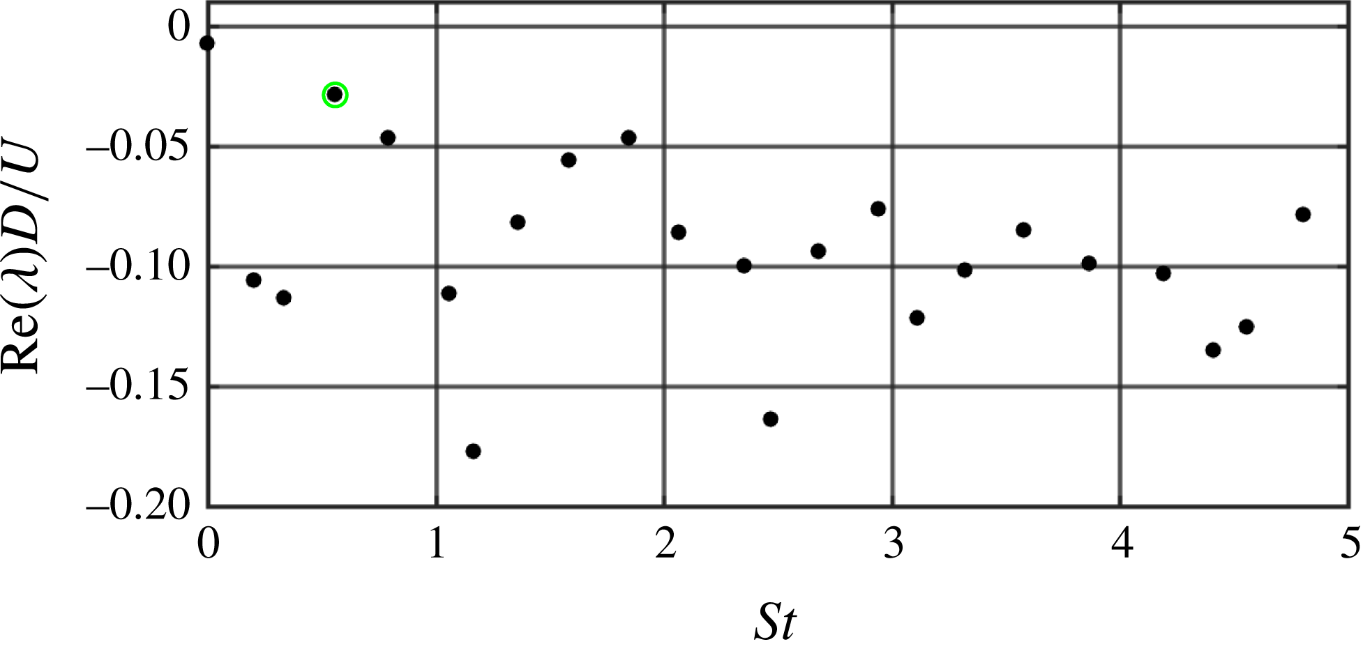
Dynamic mode spectrum in the downstream region of the jet (
 $S=0.2$
).

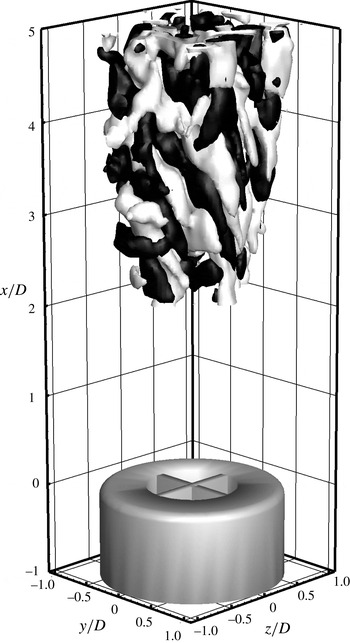
Modal representation of the vortex pairing phenomenon from the mode at
 $St=0.54$
.

In order to study the pairing phenomenon in the present configuration, the DMD analysis is performed in the downstream region of the jet starting at
 $x/D=2$
. In this region, as illustrated in figure 13, the most stable mode is at
 $St=0.54$
(highlighted with a circle in figure 13), near to 0.6, i.e. one third of the shedding frequency of the helical vortices. This supports the hypothesis that that pairing occurs in an irregular manner amongst three vortices simultaneously as can be observed in movie 1 and figure 6. The eigenvalues exhibit a greater damping than the Kelvin–Helmholtz instability (figure 12). This is consistent with the less regular behaviour observed in the instantaneous visualization. The distribution of energy over several values of the Strouhal number (0.4 and 0.8) is probably due to the pairing intermittency. However, the use of the sparsity-promoting DMD ensures that the most relevant modes are identified in this part of the flow field.
The real part of the mode corresponding to
 $St=0.54$
is visualized in figure 14 with isosurfaces of positive (in white) and negative (in black) velocity. From the representation of figure 14 the mode at
 $St=0.54$
appears to be representative of the pairing phenomenon, having black/white ribs with a period of approximately one diameter, i.e. double the period of the black/white ribs visualized in figure 12. However, the mode appears less coherent with respect to that reported in figure 12, which may be ascribed to the relatively short data sequence and the limited number of pairing events captured during the experiment.
The strength of the vortices is not azimuthally symmetric due to the azimuthal modulation and to the helical shape, which also introduce a streamwise component of the vorticity, moreover the jet broadening in the streamwise direction causes vortex stretching in the helix. The latter does not cause any more axial acceleration (deceleration) of the following (preceding) vortex. In the earlier work of Panda & McLaughlin (Reference Panda and McLaughlin1994) the pairing phenomenon was excluded in swirling jets because no evidence of it could be found from the velocity spectra measured with hot-wires on acoustically excited swirling jets. Panda and McLaughlin provided acoustic excitation to the jet in the Strouhal number range 0.75–1.5 and argued that upon interacting with the vortex breakdown, the shear layer along the jet periphery loses its organized structure and evolves towards random turbulence. In the current experiments, pairing is observed, but its behaviour is not as regular as that occurring in round jets (Violato & Scarano Reference Violato and Scarano2011) and neighbouring vortices undergo pairing with intermittency. The supplementary material (movie 1) illustrates the dynamical evolution of pairing vortices, alternately at the inner side or at the outer side of the jet. The pairing produces a lambda-shaped structure, also visualized in figures 5 and 6, at an axial distance of three diameters from the nozzle exit.
5.2 Vortex breakdown and precessing vortex core
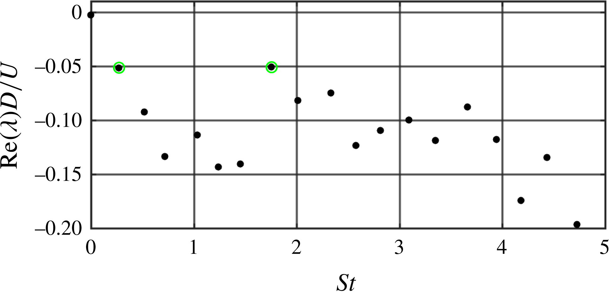
The presence of a precessing vortex core accompanied by the formation of a time-averaged reverse flow region on the jet axis is found at values of the swirl number exceeding 0.6. The data over the entire measurement domain at
 $S=0.6$
are used to extract the flow dynamic modes. The DMD spectrum is reported in figure 15: the modes which appear to be dominant are those at
 $St=0.27$
and 1.7 (highlighted with circles in figure 15). If the sparsity-promoting algorithm is applied, these two modes are found also to be those with higher amplitude.
Dynamic modes of the
 $S=0.6$
jet: dynamic mode spectrum.

Dynamic modes of the
 $S=0.6$
jet visualized with
 $Q$
criterion and (a) mode with
 $St=0.26$
, (b)
 $St=1.7$
. (c) LOR of a snapshot.

To ease the description of the phenomenon, the sparse DMD is used to provide a low-order reconstruction (LOR) of the flow field with the average field plus the contribution of the modes with
 $St=0.27$
and 1.7. The LOR and the modes are presented in figure 16. The LOR of the flow field is reported in figure 16(c) and correctly describes the flow field with the helical structures which develop in the external side of the jet and penetrate towards its centre where the strong features of the precessing vortex core and the recirculation bubble can be identified. The low-order reconstruction returns the main flow features of the jet, which further supports the choice of the DMD modes with
 $St=0.26$
and 1.7 as yielding the more representative flow structures of the flow field, despite their rather strong damping. The DMD modes at
 $St=0.26$
and 1.7 are visualized in figure 16(a,b) respectively with vortical features visualized using
 $Q$
isosurfaces coloured according to the radial distance (blue, close to the jet axis; red, towards the jet periphery). The helical vortices develop in the outer part of the jet and slowly penetrate towards its centre. At approximately 1.5 diameters from the nozzle larger vortical structures, oriented in the azimuthal direction with less pronounced helicity, appear and penetrate towards the jet centre and look like the typical structures produced in the pairing process. Both structures, when penetrating towards the jet centre, due to their pulsatile behaviour are responsible for axial gradients of azimuthal vorticity as already shown in figure 9(c), thus satisfying the Kurosaka et al. (Reference Kurosaka, Cain, Srigrarom, Wimer, Dabiri, Johnson, Hatcher, Thompson, Kikuchi, Hirano, Yugé and Honda2006) criterion for vortex breakdown. This finding confirms experimentally, for vane-generated swirling jets, the theory formulated by Brown & Lopez (Reference Brown and Lopez1990) and generalized by Kurosaka et al. (Reference Kurosaka, Cain, Srigrarom, Wimer, Dabiri, Johnson, Hatcher, Thompson, Kikuchi, Hirano, Yugé and Honda2006).
The interaction between the vortex core and the vortices developed in the shear layer has statistical evidence from figure 16. In fact surprisingly none of the two modes includes a helical vortex breakdown. The helical vortex breakdown therefore has to be ascribed to a composition of the central vortex core (in the time-averaged flow field) and the rib vortices which penetrate in the inner side of the jet. This composition contributes to achieving the breakdown and the formation of the double helix. As shown from vortex theorems in Majda & Bertozzi (Reference Majda and Bertozzi2002), two parallel vortices must then rotate about their common centre of mass at a fixed angular velocity; i.e. in this case, the two helical vortices must have a precessing motion around the recirculation region, thus justifying the vortex core precession after the breakdown.
Here, since the two helical vortices are due to the interaction between the central vortex core and rib-like vortices generated in the shear layer, the helix must follow their swirling convection with a mechanism similar to that of a corkscrew: the helix rotates while is convected downstream and the vortex core is in rotation on its axis (as shown in movie 3).
The mode with Strouhal number of 0.27 poses some questions about the reason of such a Strouhal number for the vortex core precession. Syred (Reference Syred2006) reports various Strouhal number data on PVC precession against the swirl number; these results show a dependence of
 $St$
on
 $S$
which is strongly affected by the nozzle geometry while the Reynolds number has little influence. The dependence of precession Strouhal number on the swirl number suggests that PVC is governed both by the axial shedding frequency and the fluid tangential velocity. According to the present results, the fluid tangential momentum triggers the development of the helical vortices in the jet shear layer, while the axial shedding is responsible for triggering the precession. As can be visualized in movie 3, also for
 $S=0.6$
the ‘pairing’ occurs amongst three vortices thus corresponding to a Strouhal number of approximately one third of the value for shedding. According to the illustrated mechanism of interaction between the shear layer vortices and the precessing vortex core, every pairing event corresponds to the passage of one of the two helices. Consequently, it is expected that the complete precession of the vortex core is characterized by a Strouhal number equal to approximately one sixth of the shedding Strouhal number.
6 Conclusions
This work presents a time-resolved tomographic PIV study of swirling jets issued from a nozzle with cross-helical vanes at swirl number
 $S$
ranging from 0 to 0.8 and
 $Re=1000$
.
From the observation of time-averaged flow fields it is shown that the vanes used to produce the swirl have a significant impact on the azimuthal modulation of momentum with the jet exhibiting four sectors separated by a thin wake produced by the boundary layer developed along the vane walls. Swirl causes increased jet cross-section broadening and entrainment. Further increase of the swirl number is accompanied by the appearance of a central recirculation zone due to vortex breakdown at
 $S=0.6$
. The measurement of the swirl number from the average flow field shows that equation (2.1) (Gupta et al.
Reference Gupta, Lilley and Syred1984) used to design swirl vanes is approximated; nevertheless, the error related to this formula decreases with increasing value of the swirl number down to 5 % at
 $S=0.8$
and can be considered correct enough for practical high swirl applications.
The instantaneous three-dimensional vorticity patterns show no instability development of the jet shear layer at
 $S=0$
. In contrast, the introduction of swirl enables the development of helical vortices in the jet shear layer according to Rayleigh’s stability criterion.
The helical vortices correspond to the main mode in the DMD analysis of the jet near field. The temporal inspection of the measured flow field shows the vortex pairing in the shear layer: this is not symmetric since the vortices undergo pairing alternatively in the inner and in the outer part of the shear layer. Pairing involves three vortices; as such it would be better referred to as trioing. This kind of vortex interaction is observed at all investigated values of the swirl number in contrast with previous results by Panda & McLaughlin (Reference Panda and McLaughlin1994). At higher swirl number the axial vorticity associated with the swirl velocity becomes comparable to the vorticity component due to the axial shear layer (
 $S=0.4$
) and vortex core tilting and precession occur. Further increasing the swirl number, the axial vorticity component becomes the most relevant feature of the flow field. The dynamical features at
 $S=0.6$
support the hypothesis that the precessing vortex core and the helical vortices have an interaction that enhances the breakdown and precession and suppresses the vortex pairing.
Finally, the vortex breakdown phenomenon appears to be caused by azimuthal vorticity due to helical vortices penetrating inwards through the vane’s wake. The relationship between vortex breakdown and azimuthal vorticity appears to agree with the theory by Kurosaka et al. (Reference Kurosaka, Cain, Srigrarom, Wimer, Dabiri, Johnson, Hatcher, Thompson, Kikuchi, Hirano, Yugé and Honda2006). This aspect has been confirmed by statistical evidence from the DMD analysis which, however, returns modes not corresponding to the central helix. The latter is the result of superimposing the central vortex core with the helical vortices in the inner shear layer.
Acknowledgements
The authors kindly acknowledge LaVision GmbH for PIV hardware support. The research described in this article has not been supported by the Innovation and Networks Executive Agency of the European Commission. The views expressed in this article have not been adopted or in any way approved by the European Commission and do not constitute a statement of the European Commission’s views.
Supplementary movies
Supplementary movies are available at https://doi.org/10.1017/jfm.2018.140.