



1 Introduction
It is well known that the dimension of the isometry group
 $\text {Iso}(M,g)$
of a three-dimensional pseudo-Riemannian manifold
 $(M,g)$
is at most six. If
 ${\mathrm {dim}(\text {Iso}(M,g))= 6}$
, then
 $(M,g)$
has constant curvature, and conversely. Moreover, there exist no three-dimensional pseudo-Riemannian manifolds whose isometry groups have dimension five. So, it is a natural problem to investigate three-dimensional pseudo-Riemannian manifolds
 $(M,g)$
such that
 $\mathrm {dim}(\text {Iso}(M,g))= 4$
. In these cases,
 $\text {Iso}(M,g)$
acts transitively, that is,
 $(M,g)$
is an homogeneous pseudo-Riemannian manifold.
The Riemannian case is well understood and has been extensively investigated. Three-dimensional Riemannian manifolds with four-dimensional isometry groups are known as Bianchi–Cartan–Vranceanu spaces (BCV spaces for short), because the three mathematicians contributed to their description under different perspectives. In fact, Bianchi [Reference Bianchi2, Reference Bianchi3] classified homogeneous Riemannian three-manifolds; however, Cartan [Reference Cartan11] described all four-dimensional isometry groups on Riemannian three-dimensional manifolds, introducing the following two-parameter family of Riemannian metrics (see also [Reference Vranceanu19]):
 $$ \begin{align} g^R_{\kappa,\tau}=\frac{dx^2+ dy^2}{(1+ ({\kappa}/{4})(x^2+ y^2))^2}+ \bigg(dz+\tau\frac{y\,dx-x\,dy}{(1+({\kappa}/{4})(x^2+ y^2))}\bigg)^2, \end{align} $$
where
 $(x, y, z)$
are the standard coordinates on
 ${\mathbb R}^3$
and
 ${1+ ({\kappa }/{4})(x^2+ y^2)}\neq 0$
. We set
 $\mathbb {M}^3(\kappa , \tau ) =({\mathbb R}^3, g^R_{\kappa ,\tau })$
and we recall that:
-
•
 $\mathbb {M}^3(0,0)={\mathbb R}^3$
is the Euclidean three-space;
-
•
$\mathbb {M}^3(0,\tau )$
is the Heisenberg three-space; -
•
$\mathbb {M}^3(\kappa , 0)$
is isometric to the Riemannian product
$\mathbb {M}^2(\kappa )\times {\mathbb R}$
; -
•
$\mathbb {M}^3(4\tau ^2,\tau )$
has a six-dimensional isometry group, namely, it has constant positive sectional curvature.



BCV spaces can be obtained by a fibration over a complete and simply connected surface
 $\mathbb {M}^2(\kappa )$
of constant curvature
 $\kappa \in {\mathbb R}$
, with geodesic fibres. Therefore, for each
 $\kappa $
, there is a one-parameter family
 $\mathbb {M}^3(\kappa , \tau )$
of these fibrations, parametrized by the bundle curvature
 $\tau \in {\mathbb R} - \{0\}$
.
Several authors studied the geometry of BCV spaces and many classes of their surfaces have been described. Just to mention a few examples, we may refer to [Reference Belkhelfa, Dillen and Inoguchi1] for the classification of parallel surfaces and [Reference Souam and Toubiana17] for the study of totally umbilical surfaces.
As observed in [Reference Daniel12], when
 $\tau \neq 0$
, the isometry group has two connected components, corresponding to the case where isometries preserve the orientations of both the fibres and the base of the fibration, and to the one where isometries reverse them. Consequently, we have the following possibilities:
-
• for
$\kappa>0$
,
$\text {Iso}(\mathbb {M}^3(\kappa , \tau ))=\text {Iso}(\mathbb {S}^3_{\varepsilon })$
, where
$\mathbb {S}^3_{\varepsilon }$
denote the Berger spheres; -
• for
$\kappa =0$
,
$\text {Iso}(\mathbb {M}^3(0, \tau ))=\text {Iso}(Nil_3)$
, where
$Nil_3$
is the three-dimensional Heisenberg group; -
• for
$\kappa <0$
,
$\text {Iso}(\mathbb {M}^3(\kappa , \tau ))=\text {Iso}(\widetilde {PSL_2({\mathbb R})})$
, where
$\widetilde {PSL_2({\mathbb R})}$
denotes the universal covering of the unitary tangent bundle to the hyperbolic plane equipped with its canonical metric.









In the Lorentzian case, several authors investigated relevant classes of surfaces in some particular cases corresponding to the above Riemannian ones: for example, Lorentzian Berger spheres [Reference Onnis, Passamani and Piu13] and the Heisenberg group equipped with some left-invariant Lorentzian metrics [Reference Calvaruso, Castrillón-Lopez and Pellegrino4, Reference Onnis and Piu14, Reference Turhan and Altay18]. To the best of our knowledge, a unified approach to a family of Lorentzian metrics similar to the Riemannian BCV has been considered only in the recent paper [Reference Yildirim20], where the author started with the above-mentioned fibration over a Riemannian surface
 $\mathbb {M}^2(\kappa )$
and obtained a family of homogeneous Lorentzian metrics of the form (1-1) by changing the sign before the term in the square brackets. However, this approach left out some relevant examples, namely, the ones obtained considering a Riemannian fibration on a Lorentzian source surface
 $\mathbb {M}_1^2(\kappa )$
. We refer to both these classes, that is, the one already considered in [Reference Yildirim20] and this new one, as Lorentzian Bianchi–Cartan–Vranceanu (LBCV) spaces for their evident similarity with their Riemannian analogues.
As it often occurs, the Lorentzian case is richer and subtler with respect to its Riemannian analogue. In fact, while BCV exhaust the description of Riemannian three-manifolds with four-dimensional isometry groups, there are further classes of homogeneous Lorentzian three-manifolds with such a property, as can be seen by comparing the classification of (nonisometric) homogeneous structures in the Riemannian [Reference Calviño-Louzao, Ferreiro-Subrido, Garcia-Rio and Vazquez-Lorenzo10] and the Lorentzian cases [Reference Calvaruso and Zaeim9]. This makes the study of the geometry of surfaces in homogeneous Lorentzian three-manifolds a larger programme, which we started in [Reference Calvaruso, Castrillón-Lopez and Pellegrino4, Reference Calvaruso and Pellegrino6], considering totally umbilical surfaces in the Lorentzian products and the Lorentzian metrics on
 $Nil_3$
, respectively. Moreover, parallel surfaces of all Lorentzian Lie groups were investigated in [Reference Calvaruso and Van der Veken8] (although without obtaining an explicit description for the immersions). The aim of this paper is to make substantial progress in this programme, first describing in full generality Lorentzian BCV spaces and their geometric properties, and then investigating several relevant classes of their surfaces.
The paper is organized in the following way. In Section 2, we describe Lorentzian Bianchi–Cartan–Vranceanu spaces and their geometry and recall some basic information concerning surfaces in Lorentzian ambient three-spaces. In Section 3, we study totally umbilical surfaces in Lorentzian Bianchi–Cartan–Vranceanu spaces. The main result of Section 3, namely, Theorem 3.3, shows that totally umbilical surfaces do not exist on these spaces (with the obvious exceptions when they are either direct products or of constant sectional curvature).
Parallel surfaces in Lorentzian Bianchi–Cartan–Vranceanu spaces are studied in Section 4, where Theorem 4.7 provides the complete classification and explicit description of these surfaces, which turn out to be cylinders over some suitable curves of the
 $xy$
-plane. Finally, in Section 5, we deal with constant mean curvature (CMC) and minimal surfaces in Lorentzian Bianchi–Cartan–Vranceanu spaces, characterizing them by some general equations and providing some explicit examples.
2 Preliminaries
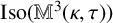
2.1 LBCV spaces
As we already mentioned in Section 1, we describe LBCV spaces by considering a fibration over some complete and simply connected surface, either Riemannian or Lorentzian, of constant curvature
 $\kappa \in {\mathbb R}$
, with geodesic fibres. Therefore, whenever we fix such a surface, there exists a one-parameter family
 $\mathbb {M}^3_1(\kappa , \tau )$
of these fibrations, parametrized by the bundle curvature
 $\tau \in {\mathbb R} -\{0\}$
. Clearly, to get a Lorentzian metric, if the surface is Riemannian, then the submersion has to be Lorentzian, and conversely.
We consider the standard coordinates
 $(x, y, z)$
on
 ${\mathbb R}^3$
. Then,
 $\mathbb {M}^3_1(\kappa , \tau )=({\mathbb R}^3, g_{\kappa ,\tau })$
, where the metrics
 $g_{\kappa ,\tau }$
are explicitly given by
 $$ \begin{align} g_{\kappa,\tau}=\frac{dx^2-\delta dy^2}{(1+ ({\kappa}/{4})(x^2-\delta y^2))^2}+\delta \bigg(dz+\tau\frac{y\,dx-x\,dy}{(1+ ({\kappa}/{4})(x^2-\delta y^2))}\bigg)^2,\quad \delta =\pm 1. \end{align} $$
The case
 $\delta =-1$
corresponds to the Lorentzian spaces already considered in [Reference Yildirim20]. To the best of our knowledge, the case
 $\delta =1$
has not been previously considered in the literature. It corresponds to the situation of a Riemannian submersion over a Lorentzian surface
 $\mathbb {M}_1^2 (\kappa )$
of constant curvature. It is relevant to observe that the above Equation (2-1) gives the opportunity to treat these two cases in a unified way.
Remark 2.1. We observe that:
-
•
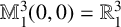
$\mathbb {M}^3_1(0,0)={\mathbb R}^3_1$
is the Minkowski three-space; -
•
$\mathbb {M}^3_1(0,\tau )$
is the Lorentzian Heisenberg three-space, equipped, depending on the sign of
$\delta $
, with its two families of nonflat left-invariant Lorentzian metrics [Reference Rahmani and Rahmani15]; -
•
$\mathbb {M}^3_1(\kappa , 0)$
is isometric to a Lorentzian product
$\mathcal {M}_\delta $
, where
$\mathcal {M}_{-1}=\mathbb {M}^2(\kappa )\times {\mathbb R}_1$
and
$\mathcal {M}_1=\mathbb {M}^2_1(\kappa )\times {\mathbb R}$
; -
•
$\mathbb {M}^3_1(-4\tau ^2, \tau )$
has constant negative sectional curvature.





As in the Riemannian case, when
 $\tau \neq 0$
, the isometry group is made up of two connected components (in both cases,
 $\delta =\pm 1$
). In particular, when
 $\delta =-1$
:
-
• for
$\kappa>0$
,
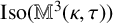
$\text {Iso}(\mathbb {M}^3(\kappa , \tau ))$
corresponds to the group of isometries of so-called Lorentzian Berger spheres (see [Reference Onnis, Passamani and Piu13]), that is, the three-dimensional spheres endowed with a one-parameter family of Lorentzian metrics, obtained by deforming the round metric on
$\mathbb {S}^3$
along the fibres of the Hopf fibration; -
• for
$\kappa <0$
,
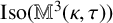
$\text {Iso}(\mathbb {M}^3(\kappa , \tau ))$
corresponds to the group of isometries of the Berger-like metrics on the anti-de Sitter space (as they appear in [Reference Calvaruso, Onnis, Pellegrino and Uccheddu5, Reference Calvaruso and Perrone7]).



However, to the best of our knowledge, the case when
 $\delta =1$
has not been previously described in this way in the literature. For
 $\delta =1$
, we have the following possibilities:
-
• for
$\kappa>0$
,
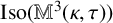
$\text {Iso}(\mathbb {M}^3(\kappa , \tau ))$
corresponds to the group of isometries of the three-dimensional sphere
$\mathbb {S}^3_1$
endowed with a deformation of its standard Lorentzian metric along the spacelike fibres of the Hopf fibration; -
• for
$\kappa <0$
,
$\text {Iso}(\mathbb {M}^3(\kappa , \tau ))$
corresponds to the group of isometries of
$SL(2, {\mathbb R})$
endowed with an analogous deformation of its standard Lorentzian metric along the spacelike direction of the fibres of the hyperbolic Hopf fibration.




From now on, we assume that
 $\mathbb {M}^3_1(\kappa , \tau )$
is not a Lorentzian product manifold
 $\mathcal {M}_\delta $
, that is,
 $\tau \neq 0$
. Starting from (2-1) and the coordinate vector fields
 ${\partial _{x}} ,{\partial _{y}} ,{\partial _{z}} $
, we then easily deduce an orthonormal basis for
 $\mathbb {M}^3_1(\kappa ,\tau )$
, namely,
 $$ \begin{align*} e_1= \Lambda {\partial_{x}}-\tau y {\partial_{z}}, \quad e_2= \Lambda {\partial_{y}}+\tau x {\partial_{z}},\quad e_3={\partial_{z}}, \end{align*} $$
where
 ${g_{\kappa , \tau }}(e_1, e_1)=1$
,
 $g_{\kappa , \tau }(e_3,e_3)=-g_{\kappa , \tau }(e_2,e_2)=\delta $
and
 $\Lambda := 1+ ({\kappa }/{4}) (x^2-\delta y^2)\neq 0$
. We have the following.
Proposition 2.2. Excluding the cases of constant sectional curvature,
 ${\mathbb {M}^3_1(\kappa ,\tau )}$
admits the following basis of complete Killing vector fields:
 $$ \begin{align*} \begin{array}{ll} X_1=\bigg(1+\delta\displaystyle\frac{\kappa y^2}{2\Lambda}\bigg) e_1+\displaystyle\frac{\kappa xy}{2\Lambda}e_2+\displaystyle\frac{2\tau y}{\Lambda}e_3, & \quad X_2=-\delta\displaystyle\frac{\kappa xy}{2\Lambda}e_1+ \bigg(1-\displaystyle\frac{\kappa x^2}{2\Lambda}\bigg)e_2-\displaystyle\frac{2\tau x}{\Lambda}e_3, \\[6pt] X_3=\delta\displaystyle\frac{y}{\Lambda}e_1+\displaystyle\frac{x}{\Lambda}e_2-\tau\displaystyle\frac{x^2-\delta y^2}{\Lambda}e_3, & \quad X_4=e_3 \end{array} \end{align*} $$
and so, the isometry group of
 $\mathbb {M}^3_1(\kappa , \tau )$
is four-dimensional.
The above result is obtained by a direct but long calculation, which we omit. However, it is straightforward to check that the above vector fields are complete Killing vector fields for the metric (2-1).
We now proceed to the description of the curvature of Lorentzian Bianchi–Cartan– Vranceanu spaces, which may be also useful for further investigations. Starting from (2-1), we prove the following.
Proposition 2.3. Consider an arbitrary Lorentzian Bianchi–Cartan–Vranceanu metric
 $g_{\kappa ,\tau }$
, as described by (2-1) in global coordinates
 $(x,y,z)=(x_1,x_2,x_3)$
. Then, with respect to the global basis
 $\{\partial _1=\partial _x, \partial _2=\partial _y, \partial _3=\partial _z \}$
of coordinate vector fields, we have the following.
-
(a) The Levi–Civita connection of
$g_{\kappa ,\tau }$
is explicitly determined by the following covariant derivatives
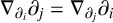
$\nabla _{{\partial _{i}}}{\partial _{j}}=\nabla _{{\partial _{j}}}{\partial _{i}}$
: (2-2)
$$ \begin{align} \begin{array}{l} \nabla_{{\partial_{1}}}{\partial_{1}}=-\displaystyle\frac{\kappa }{2\Lambda}x_1{\partial_{1}} +\displaystyle\frac{\kappa+4\tau^2}{2\Lambda} x_2{\partial_{2}}+\displaystyle\frac{\tau(\kappa+4\tau^2)}{2\Lambda^2} x_1x_2{\partial_{3}}, \\[5pt] \nabla_{{\partial_{1}}}{\partial_{2}}=\displaystyle\frac{\delta(\kappa+2\tau^2)}{2\Lambda} x_2{\partial_{1}} -\displaystyle\frac{\kappa+2\tau^2 }{2\Lambda}x_1{\partial_{2}}-\displaystyle\frac{\tau(\kappa+4\tau^2)}{4\Lambda^2} (x_1^2+\delta x_2^2){\partial_{3}}, \\[5pt] \nabla_{{\partial_{1}}}{\partial_{3}}= \tau {\partial_{2}}+\displaystyle\frac{\tau^2}{\Lambda} x_1 {\partial_{3}}, \\[5pt] \nabla_{{\partial_{2}}}{\partial_{2}}= -\displaystyle\frac{\delta(\kappa+2\tau^2) }{2\Lambda}x_1{\partial_{1}} +\displaystyle\frac{\delta\kappa }{2\Lambda} x_2 {\partial_{2}}+\displaystyle\frac{\delta\tau(\kappa+4\tau^2)}{2\Lambda^2} x_1x_2{\partial_{3}}, \\[5pt] \nabla_{{\partial_{2}}}{\partial_{3}}= \delta\tau {\partial_{1}}-\displaystyle\frac{\delta\tau^2}{\Lambda} x_2 {\partial_{3}}, \\[5pt] \nabla_{{\partial_{3}}}{\partial_{3}}= 0. \end{array} \end{align} $$
-
(b) Up to symmetries, the possibly nonvanishing components of the Riemann curvature tensor of the metric (2-1) with respect to
$\{\partial _i \}$
are given by (2-3)
$$ \begin{align} \begin{array}{lll} R_{1212}= \displaystyle\frac{\delta}{\Lambda^4} (\kappa+3\tau^2 +\tau^4(x_1^2-\delta x_2^2)), \quad & R_{1213}= \displaystyle\frac{\delta\tau^3}{\Lambda^3}x_1, \quad & R_{1223}= \displaystyle\frac{\tau^3}{\Lambda^3}x_2 , \\[5pt] R_{1313}= -\displaystyle\frac{\delta\tau^2}{\Lambda^2}, \quad & R_{2323}= \displaystyle\frac{\tau^2}{\Lambda^2}. \end{array} \end{align} $$
-
(c) The Ricci tensor
$\varrho $
of (2-1) is determined with respect to
$\{\partial _i\}$
by the following components
$\varrho _{ij} = \varrho (\partial _i , \partial _j)$
: (2-4)
$$ \begin{align} \begin{array}{lll} \varrho_{11}= \displaystyle\frac{\kappa+2\tau^2 -2\delta \tau^4 x_2^2}{\Lambda^2} , \quad & \varrho_{12}= \displaystyle\frac{2\delta \tau^4 x_1 x_2}{\Lambda^2} , \quad & \varrho_{13}= -\displaystyle\frac{2\delta \tau^3 x_2}{\Lambda} , \\[5pt] \varrho_{22}=- \displaystyle\frac{\delta(\kappa+2\tau^2 +2 \tau^4 x_1^2)}{\Lambda^2} , \quad & \varrho_{23}= \displaystyle\frac{2\delta \tau^3 x_1}{\Lambda} , \quad & \varrho_{33}= -2\delta \tau^2. \end{array} \end{align} $$
-
(d) The Ricci operator Q of (2-1) is described, in terms of the matrix of its components with respect to the basis
$\{\partial _i\}$
, by (2-5)
$$ \begin{align} Q=\left(\! \begin{array}{lll} \kappa+2\tau^2 \quad & 0 \quad & 0 \\[5pt] 0 \quad &\kappa+2\tau^2 \quad & 0 \\[5pt] - \displaystyle\frac{ \tau (\kappa+4\tau^2)x_2}{\Lambda} \quad & \displaystyle\frac{ \tau (\kappa+4\tau^2)x_1}{\Lambda} \quad & -2\tau^2 \end{array}\!\!\!\right). \end{align} $$






Proof. The equations in (2-2) are obtained by standard calculations, starting from the Lorentzian metric g described by (2-1) and applying the well-known Koszul formula. Next, from (2-2), a direct calculation yields
 $R(\partial _i,\partial _j)\partial _k$
for all indices
 $i,j,k$
, which, taking into account (2-1), determines the curvature components
 ${R_{ijkh}=g(R(\partial _i,\partial _j)\partial _k,\partial _h)}$
with respect to the basis
 $\{{\partial _{i}}\}$
of coordinate vector fields.
As it is well known, the Ricci tensor
 $\varrho $
is obtained by contraction of the curvature tensor, so that the Ricci components
 $\varrho _{ij}$
are deduced from (2-3) in a standard way. Finally, the Ricci operator Q is defined by condition
 $g(Q(X),Y)=\varrho (X,Y)$
for all tangent vector fields
 $X,Y$
. Therefore, the components of Q with respect to the basis
 $\{{\partial _{i}}\}$
of coordinate vector fields are deduced using (2-1) and (2-4).
Remark 2.4. In general, the Ricci operator of a Lorentzian metric is self-adjoint but not necessarily diagonalizable. It easily follows from (2-5) that the Ricci operator Q of an LBCV space metric (2-1) is diagonalizable. In particular, the vector field tangent to the fibres of the submersion, namely,
 $\partial _3=\partial _z$
, is always a Ricci eigenvector.
Moreover, either (2-4) or (2-5) easily imply that
 $\mathbb {M}^3_1(\kappa , \tau )$
is Einstein if and only if
 $\kappa +4\tau ^2=0$
. In this case, (being three-dimensional)
 $\mathbb {M}^3_1(\kappa , \tau )$
has constant sectional curvature
 $-2\tau ^2 <0$
and its isometry group is six-dimensional.
Next, we show how the homogeneous space
 ${\mathbb {M}^3_1(\kappa ,\tau )}$
can be realized as a three-dimensional Lorentzian Lie group, that is, a Lie group G equipped with a left-invariant Lorentzian metric. To do so, similarly to the Riemannian case investigated in [Reference Daniel12], we determine a suitable orthonormal frame
 $\{ E_1, E_2, E_3 \}$
, namely, one that diagonalizes the Ricci operator.
Starting from (2-5), a standard calculation yields the following basis of Ricci eigenvectors for the LBCV Lorentzian metrics described by (2-1).
-
• For
$\delta =1$
: (2-6)
$$ \begin{align} \begin{array}{rl} &E_1=\Lambda(\cosh(\sigma z) {\partial_{x}} +\sinh(\sigma z){\partial_{y}} )-\tau( y\cosh(\sigma z)- x\sinh(\sigma z)){\partial_{z}}; \\[6pt] &E_2=\Lambda(\sinh(\sigma z) {\partial_{x}} +\cosh(\sigma z){\partial_{y}} )+\tau( x\cosh(\sigma z)- y\sinh(\sigma z)){\partial_{z}}; \\[6pt] &E_3={\partial_{z}}. \end{array} \end{align} $$
-
• For
$\delta =-1$
: (2-7)
$$ \begin{align} \begin{array}{rl} &E_1=\Lambda(\cos(\sigma z) {\partial_{x}} +\sin(\sigma z){\partial_{y}} )-\tau(y\cos(\sigma z)-x\sin(\sigma z)){\partial_{z}}; \\[6pt] &E_2=\Lambda(-\sin(\sigma z) {\partial_{x}} +\cos(\sigma z){\partial_{y}} )+\tau( x\cos(\sigma z)+ y\sin(\sigma z)){\partial_{z}}; \\[6pt] &E_3={\partial_{z}} , \end{array} \end{align} $$


where we set
 $\sigma = {\kappa }/{2\tau }$
. In both cases,
 $E_1$
is spacelike, while
 $g_{\kappa , \tau }(E_3,E_3)=-g_{\kappa , \tau }(E_2,E_2)=\delta $
. Moreover, in both cases,
 $$ \begin{align} [E_1, E_2]=2\tau E_3, \quad [E_2, E_3]=-\delta \frac{\kappa}{2\tau} E_1, \quad [E_3, E_1]=\frac{\kappa}{2\tau} E_2. \end{align} $$
Expressions (2-8) for the Lie brackets
 $[E_i,E_j]$
of the orthonormal basis
 $\{E_i\}$
allow us to identify the corresponding Lie algebras considering the different possibilities of the parameters
 $\delta $
,
 $\kappa $
and
 $\tau $
. We have already observed that for
 $\kappa =0$
, we obtain the Lorentzian Heisenberg groups. For
 $\kappa \neq 0$
, the Lie algebras
 ${\mathbb {M}^3_1(\kappa ,\tau )}$
correspond to the following Lie groups G with a diagonal structure operator, as described in [Reference Rahmani16]:
-
• if
$\delta =1$
, then
$G=O(1,2)$
or
$G=SL(2,\mathbb {R})$
for any
$\kappa , \tau \neq 0$
; -
• if
$\delta =-1$
, then, for any
$\tau \neq 0$
:-
–
$G=O(1,2)$
or
$G=SL(2,\mathbb {R})$
if
$\kappa <0$
; -
–
$G=SO(3)$
or
$G=SU(2)$
if
$\kappa>0$
.
-




Remark 2.5. As shown in [Reference Calvaruso and Zaeim9], three-dimensional Lorentzian Lie groups, whose isometry groups are four-dimensional, form three mutually exclusive classes, which exist for some distinct forms of the self-adjoint structure operator L associated with their Lie algebras:
-
(I) Lie groups for which L is diagonal and has two distinct eigenvalues;
-
(II) an example for which the minimal polynomial of L has a nonvanishing double root;
-
(III) some homogeneous plane waves for which the minimal polynomial of L has
$0$
as a triple root.

We see from (2-8) that Lorentzian BCV spaces cover exactly the above case (I). So, in this sense, they correspond exactly to Riemannian BCV spaces. However, as we anticipated in Section 1, not all three-dimensional Lorentzian Lie groups are Lorentzian BCV spaces.
Using (2-2), (2-6) and (2-7), we get the following description of the Levi–Civita connection of
 $\mathbb {M}^3_1(\kappa , \tau )$
with respect to
 $\{E_i\}$
:
 $$ \begin{align} \begin{array}{lll} \nabla_{E_1} E_1=0, \quad & \nabla_{E_1} E_2= \tau E_3, \quad & \nabla_{E_1} E_3=\tau E_2, \\[7pt] \nabla_{E_2} E_1=-\tau E_3, \quad & \nabla_{E_2}E_2 = 0, \quad & \nabla_{E_2} E_3=\delta\tau E_1,\\[7pt] \nabla_{E_3} E_1=\displaystyle\dfrac{\kappa+2\tau^2}{2\tau} E_2, \quad & \nabla_{E_3} E_2=\delta \displaystyle\dfrac{\kappa+2\tau^2}{2\tau} E_1 , \quad & \nabla_{E_3} E_3=0. \end{array} \end{align} $$
Moreover, we observe that the Killing vector field
 $E_3$
satisfies
 $$ \begin{align} \nabla_X E_3=\delta \tau(X\wedge E_3) \end{align} $$
for all
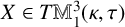 $X \in T\mathbb {M}^3_1(\kappa , \tau )$
, where the wedge product
 $\wedge $
is completely determined by
 $E_1\wedge E_2=\delta E_3$
,
 $E_2\wedge E_3=E_1$
and
 $E_3\wedge E_1=-\delta E_2$
(see [Reference Rahmani16]).
Next, starting from (2-9), we find that the Riemannian curvature tensor is completely determined by
 $$ \begin{align} \begin{split} R(E_1,E_2)E_1=-(\kappa+3\tau^2) E_2, \quad R(E_1,E_3)E_1=\tau^2 E_3, \quad R(E_2,E_3)E_2=-\delta \tau^2 E_2 \end{split} \end{align} $$
and we can prove the following result.
Proposition 2.6. The curvature tensor of
 $\mathbb {M}^3_1(\kappa , \tau )$
is given by
 $$ \begin{align*} \begin{aligned} R(X,Y)Z &=-(\kappa+3\tau^2) ({g_{\kappa, \tau}}(X,Z)Y-{g_{\kappa, \tau}}(Y,Z)X)\\ &\quad +\delta(k+4\tau^2)[{g_{\kappa, \tau}}(X,E_3){g_{\kappa, \tau}}(Z,E_3)Y-{g_{\kappa, \tau}}(Y,E_3){g_{\kappa, \tau}}(Z,E_3)X\\ &\qquad\qquad\qquad\ +{g_{\kappa, \tau}}(X,Z){g_{\kappa, \tau}}(Y,E_3)E_3-{g_{\kappa, \tau}}(Y,Z){g_{\kappa, \tau}}(X,E_3)E_3] \end{aligned} \end{align*} $$
for all tangent vector fields
 $X,Y,Z$
.
Proof. Consider three arbitrary vector fields
 $X, Y, Z$
on
 $\mathbb {M}^3_1(\kappa , \tau )$
and their decompositions as
 $$ \begin{align*} X=\bar{X}+xE_3, \quad Y=\bar{Y}+yE_3, \quad Z=\bar{Z}+zE_3, \end{align*} $$
with
 $\bar {X}, \bar {Y}, \bar {Z}$
orthogonal to
 $E_3$
and
 $x=\delta {g_{\kappa , \tau }}(X,E_3)$
, and so on. Observe that using (2-11), we have that all terms of
 ${g_{\kappa , \tau }}(R(X,Y)Z,W)$
, where
 $E_3$
occurs either one, three or four times, necessarily vanish. Therefore,
 $$ \begin{align*} \begin{split} {g_{\kappa, \tau}}(R(X,Y)Z,W)&={g_{\kappa, \tau}}(R(\bar{X},\bar{Y})\bar{Z},\bar{W})\\ &\quad +xz{g_{\kappa, \tau}}(R(E_3,\bar{Y})E_3,\bar{W})+yz{g_{\kappa, \tau}}(R(\bar{X},E_3)E_3,\bar{W})\\ &\quad +yw{g_{\kappa, \tau}}(R(\bar{X},E_3)\bar{Z},E_3)+xw{g_{\kappa, \tau}}(R(E_3,\bar{Y})\bar{Z},E_3). \end{split} \end{align*} $$
From the decompositions of
 $\bar {X}$
,
 $\bar {Y}$
,
 $\bar {Z}$
and
 $\bar {W}$
, it follows that
 $$ \begin{align*} \begin{split} {g_{\kappa, \tau}}(R(\bar{X},\bar{Y})\bar{Z},\bar{W})=-(k+3\tau^2)({g_{\kappa, \tau}}(\bar{X},\bar{Z}){g_{\kappa, \tau}}(\bar{Y},\bar{W})-{g_{\kappa, \tau}}(\bar{X},\bar{W}){g_{\kappa, \tau}}(\bar{Y},\bar{Z})). \end{split} \end{align*} $$
Moreover,
 $$ \begin{align*} R(\bar{X}, E_3)E_3=-\delta\tau^2\bar{X},\quad R(E_3,\bar{Y})E_3=\delta\tau^2 \bar{Y}. \end{align*} $$
Hence, we conclude that
 $$ \begin{align*} &{g_{\kappa, \tau}}(R(X,Y)Z,W)=-(k+3\tau^2)({g_{\kappa, \tau}}(\bar{X},\bar{Z}){g_{\kappa, \tau}}(\bar{Y},\bar{W})-{g_{\kappa, \tau}}(\bar{X},\bar{W}){g_{\kappa, \tau}}(\bar{Y},\bar{Z}))\\ &\qquad +\delta \tau^2 (xz{g_{\kappa, \tau}}(\bar{Y},\bar{W})-yz {g_{\kappa, \tau}}(\bar{X},\bar{W})+yw{g_{\kappa, \tau}}(\bar{X},\bar{Z})-xw{g_{\kappa, \tau}}(\bar{Y},\bar{Z}))\\ &\quad=-(k+3\tau^2)({g_{\kappa, \tau}}({X},{Z}){g_{\kappa, \tau}}({Y},{W})-{g_{\kappa, \tau}}({X},{W}){g_{\kappa, \tau}}({Y},{Z}))\\ &\qquad +\delta(\kappa+4\tau^2) ({g_{\kappa, \tau}}({Y},{W}){g_{\kappa, \tau}}(X,E_3){g_{\kappa, \tau}}(Z,E_3)-{g_{\kappa, \tau}}({X},{W}){g_{\kappa, \tau}}(Y,E_3){g_{\kappa, \tau}}(Z,E_3)\\ &\qquad\qquad\qquad\quad\, +{g_{\kappa, \tau}}({X},{Z}){g_{\kappa, \tau}}(Y,E_3){g_{\kappa, \tau}}(W,E_3)-{g_{\kappa, \tau}}({Y},{Z}){g_{\kappa, \tau}}(X,E_3){g_{\kappa, \tau}}(W,E_3))\\ &\quad={g_{\kappa, \tau}}(-(k+3\tau^2)({g_{\kappa, \tau}}({X},{Z})Y-{g_{\kappa, \tau}}({Y},{Z})X)\\ &\qquad +\delta(\kappa+4\tau^2) [{g_{\kappa, \tau}}(X,E_3){g_{\kappa, \tau}}(Z,E_3)Y-{g_{\kappa, \tau}}(Y,E_3){g_{\kappa, \tau}}(Z,E_3)X\\ &\qquad\qquad\qquad\quad\, +{g_{\kappa, \tau}}({X},{Z}){g_{\kappa, \tau}}(Y,E_3)E_3-{g_{\kappa, \tau}}({Y},{Z}){g_{\kappa, \tau}}(X,E_3)E_3], W), \end{align*} $$
which ends the proof, as W is arbitrary.
2.2 Geometry of surfaces in a three-dimensional Lorentzian ambient space
Consider an isometric immersion
 $F: \Sigma \to M$
, where
 $(\Sigma , g^\Sigma )$
is a pseudo-Riemannian surface embedded within a pseudo-Riemannian manifold
 $(M, g)$
of dimension three and
 $g^\Sigma $
is the metric induced by g under the map F. A unit normal vector field N on
 $\Sigma $
satisfies
 $g(N, N) = \varepsilon $
, where
 $\varepsilon = \pm 1$
. When
 $\varepsilon = 1$
, N is spacelike, making
 $\Sigma $
a timelike surface and the immersion Lorentzian. Conversely, if
 $\varepsilon = -1$
, then N is timelike,
 $\Sigma $
is a spacelike surface and the immersion is Riemannian.
Let
 $\nabla ^\Sigma $
and
 ${\nabla }$
denote the Levi–Civita connections on
 $\Sigma $
and M, respectively. For any vector fields X and Y on
 $\Sigma $
, the relationship between these connections is given by the well-known Gauss formula
 $$ \begin{align} {\nabla}_X Y = \nabla^\Sigma_X Y + h(X,Y)N, \end{align} $$
where the symmetric bilinear form h on
 $T\Sigma $
is the second fundamental form associated to the immersion F.
In general, specific properties of h characterize different classes of submanifolds. For instance, a point
 $p \in \Sigma $
is called a totally umbilical point if there exists a real number
 $\lambda (p)$
such that
 $$ \begin{align*} h(X_p, Y_p) = \lambda(p) g^\Sigma_p(X_p, Y_p). \end{align*} $$
Moreover, if every point
 $p \in \Sigma $
is totally umbilical, then
 $\Sigma $
itself is said to be totally umbilical. This means that at each point of
 $\Sigma $
, there exists a neighbourhood
 $U \subseteq \Sigma $
and a function
 $\lambda : U \rightarrow \mathbb {R}$
such that
 $$ \begin{align} h(X, Y) = \lambda g^\Sigma(X, Y) \end{align} $$
for all vector fields
 $X, Y$
on
 $T\Sigma $
. Equivalently, this condition implies that the shape operator S is a scalar multiple of the identity, so that
 $S = \lambda \, \text {Id}$
. In particular, if
 $\lambda = 0$
in (2-13), the second fundamental form h vanishes identically and, thus,
 $\Sigma $
is totally geodesic.
A different generalization of the well-known totally geodesic property is given by the parallelism condition. A surface is said to be parallel if
 $$ \begin{align*} \nabla h = 0, \end{align*} $$
which implies that all extrinsic invariants derived from h are covariantly constant.
Next, weakening the parallelism condition, one considers
 $R^\Sigma $
and
 ${R}$
the Riemann– Christoffel curvature tensors of
 $\Sigma $
and M, respectively, and defines an immersion to be semi-parallel if
 $R^\Sigma \cdot h = 0$
, where
 $$ \begin{align*} (R^\Sigma\cdot h)(X,Y,Z,W)=-h(R^\Sigma(X,Y)Z,W)-h(Z,R^\Sigma(X,Y)W) \end{align*} $$
for all vector fields
 $X, Y, Z, W \in T\Sigma $
.
In the particular case of a surface in a three-dimensional ambient space, the following interesting relationship holds between semi-parallel surfaces and the totally umbilical ones.
Lemma 2.7 [Reference Calvaruso and Van der Veken8].
In a Lorentzian three-manifold
 $(M, g)$
, any parallel surface is semi-parallel. Moreover, a surface
 $\Sigma $
in a Lorentzian manifold is semi-parallel if and only if it is either flat or totally umbilical.
The Gauss and Codazzi equations describe further conditions on
 $\Sigma $
, given by
 $$ \begin{align} & g(R(X, Y)Z, W) = g(R^\Sigma(X, Y)Z, W) + \varepsilon ( h(X, Z) h(Y, W) - h(X, W) h(Y, Z)),\notag \\ & g(R(X, Y)Z, N) = \varepsilon ( (\nabla h)(X, Y, Z) - (\nabla h)(Y, X, Z)), \end{align} $$
where X, Y, Z and W are vector fields tangent to
 $\Sigma $
.
We say that the second fundamental form h satisfies the Codazzi condition if
 $\nabla h$
is totally symmetric. It is clear from (2-14) that this property is satisfied by parallel hypersurfaces and is equivalent to
 $R(X, Y)N = 0$
for all vector fields
 $X, Y$
on
 $\Sigma $
.
In the study of submanifolds, minimal and CMC surfaces are of particular interest. The mean curvature H of a surface
 $\Sigma $
in a three-dimensional ambient space M is defined by
 $$ \begin{align*} H=\frac{1}{2}\mathrm{tr}_{g^\Sigma} h=\frac{1}{2}\sum (g^{\Sigma})^{ij}h_{ij}, \end{align*} $$
where
 $(g^{\Sigma })^{ij}$
are the components of
 $(g^\Sigma )^{-1}$
with respect to a chosen basis for the tangent space of
 $\Sigma $
. A surface is said to be minimal if
 $H = 0$
(timelike surfaces with
 $H=0$
are also referred to as maximal) and a CMC if H is constant. Clearly, totally geodesic surfaces are minimal and minimal surfaces are CMC.
3 Nonexistence of totally umbilical surfaces in LBCV spaces
In this section, we investigate the existence of totally umbilical surfaces in Lorentzian Bianchi–Cartan–Vranceanu spaces
 $\mathbb {M}^3_1(\kappa , \tau )$
. As the case of Lorentzian direct products (where such surfaces exist) was already studied in [Reference Calvaruso and Pellegrino6], we assume
 $\tau \neq 0$
, so that we can use the results of Section 2.1. Moreover, we assume
 $\kappa +4\tau ^2 \neq 0$
to exclude the case of constant sectional curvature and a six-dimensional isometry group.
Let
 $\Sigma $
denote any oriented surface immersed into
 $\mathbb {M}^3_1(\kappa , \tau )$
and N its
 $\varepsilon -$
unit normal vector field (
 ${g_{\kappa , \tau }}(N,N)={\varepsilon }$
). The vector field
 $E_3$
decomposes as
 $$ \begin{align*} E_3=T+\nu N, \end{align*} $$
where
 $\nu :=\varepsilon {g_{\kappa , \tau }}(N,E_3)$
and T is tangent to
 $\Sigma $
, whence
 $$ \begin{align*} {g_{\kappa, \tau}}(T,T)=\delta-{\varepsilon}\nu^2. \end{align*} $$
Example 3.1. The Killing vector field
 $E_3=\partial _z$
is parallel to the fibres of the Hopf fibration, which defines the spaces
 $\mathbb {M}^3_1(\kappa , \tau )$
for every
 $\kappa $
. When
 $\nu =0$
,
 $E_3$
is fully tangent to the surface
 $\Sigma $
. In this case, such a special surface ‘wraps around’ this direction, so it is called a Hopf tube.
Using the notation we introduced, the following result easily follows from Proposition 2.6.
Corollary 3.2. For any
 $X,Y$
tangent to
 $\Sigma $
:
 $$ \begin{align} R(X,Y)N =\delta\varepsilon \nu (k+4\tau^2)[{g_{\kappa, \tau}}(X,T)Y-{g_{\kappa, \tau}}(Y,T)X]. \end{align} $$
We now prove the following.
Theorem 3.3. Whenever
 $\tau \neq 0$
and
 $\kappa +4\tau ^2\neq 0$
, a Lorentzian Bianchi–Cartan– Vranceanu space
 $\mathbb {M}^3_1(\kappa , \tau )$
does not admit any totally umbilical surfaces (in particular, any totally geodesic surfaces).
Proof. Let
 $\Sigma $
be a totally umbilical surface immersed in
 $\mathbb {M}^3_1(\kappa ,\tau )$
with unit normal N such that
 ${g_{\kappa , \tau }}(N,N)=\varepsilon $
. Let
 $F: \Omega \rightarrow \mathbb {M}^3_1(\kappa , \tau )$
,
 $(u,v)\mapsto F(u,v)=(x(u,v), y(u,v), z(u,v))$
denote the (local) immersion with local coordinates
 $(u,v)$
defined on an open set
 $\Omega $
of
 ${\mathbb R}^2$
. As
 $\Sigma $
is totally umbilical, there exists a function
 $\lambda : \Omega \rightarrow {\mathbb R}$
such that
 $$ \begin{align*} \nabla_{X_u} N=-SX_u=-\lambda X_u, \quad \nabla_{X_v} N=-SX_v=-\lambda X_v. \end{align*} $$
Therefore,
 $$ \begin{align} R (X_u, X_v)N&=\nabla_{X_u} \nabla_{X_v}N- \nabla_{X_v} \nabla_{X_u}N=-\nabla_{X_u} (\lambda X_v) + \nabla_{X_v} (\lambda X_u)\notag\\[5pt] &=- \lambda_u X_v+\lambda_v X_u. \end{align} $$
However, by (3-1),
 $$ \begin{align} R(X_u,X_v)N =\delta\varepsilon \nu (\kappa+4\tau^2)[{g_{\kappa, \tau}}(X_u,T)X_v-{g_{\kappa, \tau}}(X_v,T)X_u]. \end{align} $$
Therefore, comparing (3-2) and (3-3),
 $$ \begin{align} \nabla^\Sigma \lambda=\delta {\varepsilon} \nu (\kappa+4\tau^2)T, \end{align} $$
where
 $\nabla ^\Sigma $
denotes the gradient of
 $\lambda $
on
 $\Sigma $
.
Observe that if T vanishes identically on a nonempty open set, we can choose
 ${N=E_3}$
on this set. Consequently,
 ${\varepsilon }=\delta $
and
 $\Sigma $
is spacelike (respectively timelike) if
 $\delta =-1$
(
 $\delta =1$
); moreover, using (2-10),
 $$ \begin{align*} \nabla _{X_u} N=\nabla _{X_u} E_3=\delta \tau (X_u \wedge E_3) \end{align*} $$
and we deduce that this surface cannot be totally umbilical, as it excludes the possibility that
 $\nabla _{X_u}N=\lambda X_u$
. Therefore, we can assume that T does not vanish on the given set.
As a consequence, if we suppose that
 $\lambda =0$
, from (3-4), we deduce that
 $\nu =0$
, that is,
 $T=E_3$
. Therefore, there exist some real functions a and b on
 $\Omega $
such that
 $N=aE+bE_2$
and
 $a^2-\delta b^2={\varepsilon }$
. Consequently, the vector fields
 $E_3$
and
 $V=bE_1+\delta a E_2$
span the tangent space to
 $\Sigma $
and, from
 $$ \begin{align*} 0=\lambda V=-\nabla_VN=-V(a)E_1-V(b)E_2-{\varepsilon}\delta \tau E_3, \end{align*} $$
we find a contradiction since
 $\tau \neq 0$
. Thus, there are no totally geodesic surfaces in
 $\mathbb {M}^3_1(\kappa , \tau )$
for
 $\tau \neq 0$
.
Next, we set
 $JX:=N\wedge X$
, which satisfies
 $$ \begin{align*} {g_{\kappa, \tau}} (JX,JY)=-{\varepsilon}\,{g_{\kappa, \tau}}(X, Y),\quad J^2X={\varepsilon}\, X, \end{align*} $$
for any vector fields
 $X,Y$
tangent to
 $\Sigma $
. As a consequence,
 $JT{\kern-1pt}={\kern-1pt}N{\kern-1pt}\wedge{\kern-1pt} (E_3-\nu N){\kern-1pt}={\kern-1pt}N{\kern-1pt}\wedge{\kern-1pt} E_3$
is tangent to
 $\Sigma $
and horizontal.
We can now calculate
 $$ \begin{align*} \nabla_{JT} T&=\nabla_{JT}(E_3-\nu N)\\ &=\delta \tau\,(JT\wedge E_3)-JT(\nu)N+\nu \lambda JT\\ &=-\delta \tau\, ((T+\nu N)\wedge JT)- JT(\nu)N+\nu \lambda JT\\ &=-\delta \tau\, (T\wedge JT)-{\varepsilon} \delta \nu\tau T - {\varepsilon}\delta \tau {g_{\kappa, \tau}}(N,JT\wedge E_3)N+\nu \lambda JT\\ &=-{\varepsilon} \delta \nu\tau T +\nu \lambda JT, \end{align*} $$
where we use
 $$ \begin{align*} JT(\nu)N&={\varepsilon} JT({g_{\kappa, \tau}}(N,E_3))N\\ &={\varepsilon}{g_{\kappa, \tau}}(\nabla_{JT}N, E_3)N+{\varepsilon}{g_{\kappa, \tau}}(\nabla_{JT}E_3,N)N\\ &=-\delta\tau {g_{\kappa, \tau}}(T,T)N\\ &=-\delta \tau (T\wedge JT). \end{align*} $$
Moreover,
 $$ \begin{align*} \nabla_{JT} JT&=\nabla_{JT}(N\wedge T)\\ &=(\nabla_{JT} N)\wedge T+ N\wedge (\nabla_{JT} T)\\ &=-\lambda (JT\wedge T)-{\varepsilon} \delta \nu\tau T +\nu \lambda JT. \end{align*} $$
Therefore,
 $h(JT, JT)={\varepsilon }\lambda g(T,T)$
. If we require total umbilicity, we then get
 $$ \begin{align*} \lambda {\varepsilon} {g_{\kappa, \tau}}(T,T)=\lambda{g_{\kappa, \tau}}(JT,JT)=-\lambda{\varepsilon} {g_{\kappa, \tau}}(T,T), \end{align*} $$
that is,
 ${g_{\kappa , \tau }}(T,T)={g_{\kappa , \tau }}(JT,JT)=0$
as
 $\lambda \neq 0$
. Since
 $T\neq 0$
, we find that
 $g^\Sigma \equiv 0$
and so,
 $\Sigma $
is degenerate. Thus, we conclude that there are no totally umbilical surfaces in
 $\mathbb {M}^3_1(\kappa , \tau )$
.
Remark 3.4. The results on totally umbilical surfaces obtained in Theorem 3.3 are coherent with:
-
• the nonexistence result of such surfaces in the Lorentzian Heisenberg group [Reference Calvaruso, Castrillón-Lopez and Pellegrino4];
-
• the existence of these surfaces in the reducible case (
$\tau =0$
), investigated in [Reference Calvaruso and Pellegrino6].

4 Parallel and semi-parallel surfaces in LBCV spaces
The following characterization was obtained in [Reference Calvaruso and Van der Veken8] for semi-parallel surfaces in three-dimensional manifolds.
Lemma 4.1 [Reference Calvaruso and Van der Veken8].
A surface in a three-dimensional Lorentzian manifold is semi-parallel if and only if it is either flat or totally umbilical.
Consequently, by Theorem 3.3, we have at once the following.
Corollary 4.2. Let
 $\Sigma $
be a surface immersed into a Lorentzian BCV space
 $\mathbb {M}^3_1(\kappa ,\tau )$
. When
 $\tau , \kappa +4\tau ^2\neq 0$
,
 $\Sigma $
is semi-parallel if and only if it is flat.
Every parallel surface
 $\mathbb {M}^3_1(\kappa ,\tau )$
(
 $\tau , \kappa +4\tau ^2\neq 0$
), being semi-parallel, is flat. We now classify and explicitly describe parallel surfaces of these spaces.
Let
 $F: \Sigma \rightarrow \mathbb {M}^3_1(\kappa ,\tau )$
denote the immersion of a surface
 $\Sigma $
into an LBCV space and N the unit normal vector field to the surface. We first determine some necessary algebraic conditions on the components of N with respect to the frame
 $\{E_1, E_2, E_3 \}$
on
 $\mathbb {M}^3_1(\kappa ,\tau )$
for
 $\Sigma $
to have a Codazzi second fundamental form. We prove the following.
Theorem 4.3. Every surface
 $\Sigma $
in
 $\mathbb {M}^3_1(\kappa ,\tau )$
with a Codazzi second fundamental form is isometric to a Hopf tube around the z-axis.
In fact, denoting by N the unit normal vector field to
 $\Sigma $
, with
 $ g_{\kappa , \tau }(N, N) =\varepsilon \in \{-1, 1\}$
, and considering the vector fields
 $\{E_i\}$
on
 $\mathbb {M}^3_1(\kappa ,\tau )$
described either in (2-6) or in (2-7) (depending on the value of
 $\delta $
), every point of
 $\Sigma $
admits an open neighbourhood in
 $\Sigma $
, where
 $N= a E_1+b E_2$
, for some smooth functions
 $a,b$
on
 $\Sigma $
.
Proof. Consider
 $N= a E_1+b E_2+c E_3$
for some functions
 $a, b, c: U\rightarrow {\mathbb R}$
such that
 $g_{\kappa , \tau }(N,N)=a^2-\delta (b^2-c^2)=\varepsilon =\pm 1 \neq 0$
. Then, the following vector fields are tangent to the hypersurface:
 $$ \begin{align*} X_1=b E_1+\delta aE_2, \quad X_2=c E_1-\delta aE_3, \quad X_3=c E_2+bE_3. \end{align*} $$
If h is Codazzi, then (2-14) yields that
 $R(X_i,X_j)N=0$
for every
 $i,j\in \{1,2,3\}$
. In particular,
 $$ \begin{align*} 0=R(X_2,X_3)N=-\delta c^2(\kappa+4\tau^2) X_4, \end{align*} $$
whence,
 $c=0$
and so, the direction
 $E_3={\partial _{z}}$
is fully tangent to the surface. Thus, we conclude that
 $\Sigma $
is isometric to an Hopf tube around the z-axis.
We now proceed to classify and describe parallel surfaces in
 $\mathbb {M}^3_1(\kappa ,\tau )$
. We observe that
 $g_{\kappa , \tau }(N,N)=a^2-\delta b^2$
. So, if
 $\delta =1$
, then
 $\Sigma $
can be either timelike or spacelike. However, when
 $\delta =-1$
, we necessarily have
 ${\varepsilon }=1$
. Consequently, we consider separately two cases, depending on the sign of
 $\delta $
.
Case A:
 ${\delta =1}$
. In this case,
 $N=aE_1+bE_2$
, where a and b are smooth functions on
 $\Sigma $
. As
 $g_{\kappa , \tau }(N,N)=a^2-\delta b^2={\varepsilon }$
, there exists a smooth function
 $\theta $
on
 $\Sigma $
, such that
 ${a=\cosh \theta }$
(respectively
 $\sinh \theta $
) and
 $b=\sinh \theta $
(respectively
 $\cosh \theta $
) if
 ${\varepsilon }=1$
(respectively
 $-1$
). Moreover, the vector fields
 $$ \begin{align} Y_1=b E_1+aE_2, \quad Y_2=E_3 \end{align} $$
span the tangent space to
 $\Sigma $
at every point.
A direct calculation, using (4-1) and (2-9), yields
 $$ \begin{align*} \nabla_{Y_1}Y_1=Y_1(\theta)N, \quad \nabla_{Y_2}Y_1=\bigg(Y_2(\theta)+\frac{\kappa+2\tau^2}{2\tau}\bigg)N,\quad \nabla_{Y_1}Y_2=\tau N, \quad \nabla_{Y_2}Y_2=0. \end{align*} $$
Observe that
 $\nabla ^\Sigma _{Y_i} Y_j=0$
for all indices
 $i,j$
corresponding to the fact that
 $\Sigma $
is flat. Moreover, since they commute, the vector fields
 $$ \begin{align} Y_1 = {\partial_{u}} , \quad Y_2 = {\partial_{v}} \end{align} $$
may be taken as coordinate vector fields on
 $\Sigma $
. Then, requiring that
 $h(Y_1,Y_2)=h(Y_2,Y_1)$
,
 $$ \begin{align*} {\partial_{v}}(\theta)=Y_2(\theta)=-\frac{\kappa}{2\tau}, \end{align*} $$
and so,
 $\theta (u,v)=- ({\kappa }/{2\tau })v+f(u)$
for some smooth function f depending only on u.
Next, using the Gauss formula (2-12), we get that the second fundamental form h is completely determined by
 $$ \begin{align} h(Y_1,Y_1)={\varepsilon} {\partial_{u}}(\theta)={\varepsilon} f'(u), \quad h(Y_1,Y_2)=h(Y_2,Y_1)={\varepsilon} \tau,\quad h(Y_2,Y_2)=0. \end{align} $$
Remark 4.4. Consistently with Theorem 3.3, this space does not admit any totally geodesic surfaces, as
 $h(Y_1,Y_2)=h(Y_2,Y_1)={\varepsilon } \tau \neq 0$
.
In particular,
 $\Sigma $
is parallel if and only if
 $f"(u)=0$
, that is,
 $$ \begin{align} \theta(u,v)=\alpha u+\beta-\frac{\kappa}{2\tau}v \end{align} $$
for some real constants
 $\alpha $
and
 $\beta $
.
Denote now by
 $F: \Sigma \rightarrow \mathbb {M}^3_1(\kappa ,\tau ) \; (u,v)\mapsto (x(u,v), y(u,v),z(u,v))$
the immersion of the surface
 $\Sigma $
in the local coordinates introduced above. By (4-1) and (4-2),
 $$ \begin{align} \begin{aligned} {\partial_{v}} x(u,v)=0, \ {\partial_{u}} x(u,v)&=\Lambda \bigg( b\cosh \bigg(\frac{\kappa}{2\tau}z(u,v)\bigg)+a\sinh\bigg(\frac{\kappa}{2\tau}z(u,v) \bigg)\bigg), \\[6pt] {\partial_{v}} y(u,v)=0, \ {\partial_{u}} y(u,v)&=\Lambda \bigg( b\sinh \bigg(\frac{\kappa}{2\tau}z(u,v)\bigg)+a\cosh\bigg(\frac{\kappa}{2\tau}z(u,v)\bigg)\bigg), \\[6pt] {\partial_{v}} z(u,v)=1, \ {\partial_{u}} z(u,v)&=-\tau b\bigg( y(u,v)\cosh \bigg(\frac{\kappa}{2\tau}z(u,v)\bigg)-x(u,v)\sinh\bigg(\frac{\kappa}{2\tau}z(u,v)\bigg)\bigg) \\[6pt] &\quad +\tau a\bigg(x(u,v)\cosh\bigg(\frac{\kappa}{2\tau}z(u,v)\bigg)-y(u,v)\sinh\bigg(\frac{\kappa}{2\tau}z(u,v)\bigg)\bigg). \end{aligned} \end{align} $$
Integrating (4-5), we obtain
 $x=x(u)$
,
 $y=y(u)$
and
 $z(u,v)=v+g(u)$
, with
 $$ \begin{align*} g'(u)=\frac{\tau}{\Lambda}(x(u)y'(u)-y(u)x'(u)). \end{align*} $$
To integrate the above equation, from now on, we consider separately two cases, depending on
 ${\varepsilon }=\pm 1$
.
Case A.1:
 ${\delta ={\varepsilon }=1}$
. In this case,
 $$ \begin{align*} \begin{cases} a=\cosh\theta(u,v)=\cosh\bigg(\alpha u+\beta-\displaystyle\frac{\kappa}{2\tau}v\bigg),\\[6pt] b=\sinh\theta(u,v)=\sinh\bigg(\alpha u+\beta-\displaystyle\frac{\kappa}{2\tau}v\bigg). \end{cases} \end{align*} $$
Using these relations in (4-5),
 $$ \begin{align} \begin{aligned} x'(u)&=\Lambda\sinh\bigg(\alpha u+\beta+\frac{\kappa}{2\tau}g(u)\bigg),\\[6pt] y'(u)&=\Lambda\cosh\bigg(\alpha u+\beta+\frac{\kappa}{2\tau}g(u)\bigg),\\[6pt] g'(u)&=\tau\bigg[x(u)\cosh\bigg(\alpha u+\beta+\frac{\kappa}{2\tau}g(u)\bigg)-y(u)\sinh\bigg(\alpha u+\beta+\frac{\kappa}{2\tau}g(u)\bigg)\bigg]. \end{aligned} \end{align} $$
We now derive
 $g'(u)$
. By (4-6),
 $$ \begin{align*} g"(u)&=\tau \bigg(\alpha +\frac{\kappa}{2\tau}g'(u)\bigg)\bigg[x(u)\sinh\bigg(\alpha u+\beta+\frac{\kappa}{2\tau}g(u)\bigg)-y(u)\cosh\bigg(\alpha u+\beta+\frac{\kappa}{2\tau}g(u)\bigg)\bigg]\\[6pt] &=\tau \bigg(\alpha +\frac{\kappa}{2\tau}g'(u)\bigg)\frac{x(u)x'(u)-y(u)y'(u)}{\Lambda}\\[6pt] &=\bigg(\alpha +\frac{\kappa}{2\tau}g'(u)\bigg)\frac{2\tau}{\kappa}\frac{{\partial_{u}} (\Lambda)}{\Lambda}, \end{align*} $$
where
 $\Lambda $
stands for
 $\Lambda \circ F=\Lambda (x(u),y(u))$
. Therefore,
 $x(u)x'(u)-y(u)y'(u)= ({2}/{\kappa }) {\partial _{u}} (\Lambda )$
. Moreover, by integration,
 $$ \begin{align*} \alpha+\frac{\kappa}{2\tau}g'(u)=\phi\Lambda(x(u),y(u)) \end{align*} $$
for some positive constant
 $\phi $
. Explicitly,
 $$ \begin{align*} g(u)=-\frac{2\tau \alpha}{\kappa}u+\frac{2\tau \phi}{\kappa}\int_c^u \Lambda(x(s),y(s))\,ds. \end{align*} $$
Next, setting
 $\psi (u):=\int _c^u \Lambda (x(s),y(s))\,ds$
, we rewrite the first two equations in (4-6) as
 $$ \begin{align*} x'(u)=\psi'(u)\sinh(\beta+\phi\psi(u)),\quad y'(u)=\psi'(u)\cosh(\beta+\phi\psi(u)). \end{align*} $$
Integrating,
 $$ \begin{align*} x(u)=\frac{1}{\phi}\cosh(\beta+\phi\psi(u)),\quad y(u)=\frac{1}{\phi}\sinh(\beta+\phi\psi(u)). \end{align*} $$
Therefore, the immersion F is explicitly given by
 $$ \begin{align} F(u,v)=\bigg(\frac{1}{\phi}\cosh(\beta+\phi\psi(u))+c_1,\frac{1}{\phi}\sinh(\beta+\phi\psi(u))+c_2, v-\frac{2\tau \alpha}{\kappa}u+\frac{2\tau \phi}{\kappa}\psi(u)\bigg) \end{align} $$
for some real constants
 $c_1$
and
 $c_2$
.
Case A.2:
 ${\delta =-{\varepsilon }=1}$
. This case is completely analogous to the previous case, but now,
 $$ \begin{align*} \begin{cases} a=\cosh\theta(u,v)=\sinh\bigg(\alpha u+\beta-\displaystyle\frac{\kappa}{2\tau}v\bigg),\\[6pt] b=\sinh\theta(u,v)=\cosh\bigg(\alpha u+\beta-\displaystyle\frac{\kappa}{2\tau}v\bigg). \end{cases} \end{align*} $$
Therefore, (4-5) now rewrites as
 $$ \begin{align} \begin{aligned} x'(u)&=\Lambda\cosh\bigg(\alpha u+\beta+\frac{\kappa}{2\tau}g(u)\bigg),\\[6pt] y'(u)&=\Lambda\sinh\bigg(\alpha u+\beta+\frac{\kappa}{2\tau}g(u)\bigg),\\[6pt] g'(u)&=\tau\bigg[x(u)\sinh\bigg(\alpha u+\beta+\frac{\kappa}{2\tau}g(u)\bigg)-y(u)\cosh\bigg(\alpha u+\beta+\frac{\kappa}{2\tau}g(u)\bigg)\bigg]. \end{aligned} \end{align} $$
We proceed as in the previous case, first deriving with respect to u the expression for
 $g'(u)$
in (4-8) and then integrating. We obtain
 $$ \begin{align*} g(u)=-\frac{2\tau \alpha}{\kappa}u+\frac{2\tau \phi}{\kappa}\int_c^u \Lambda(x(s),y(s))\,ds \end{align*} $$
for some positive constant
 $\phi $
. Setting
 $\psi (u):=\int _c^u \Lambda (x(s),y(s))\,ds$
, we rewrite (4-8) as
 $$ \begin{align*} x'(u)=\psi'(u)\cosh(\beta+\phi\psi(u)),\quad y'(u)=\psi'(u)\sinh(\beta+\phi\psi(u)). \end{align*} $$
Therefore, now the immersion F is given by
 $$ \begin{align} F(u,v)=\bigg(\frac{1}{\phi}\sinh(\beta+\phi\psi(u)) + c_1,\frac{1}{\phi}\cosh (\beta+\phi\psi(u))+c_2, v-\frac{2\tau \alpha}{\kappa}u+\frac{2\tau \phi}{\kappa}\psi(u)\bigg) \end{align} $$
for some real constants
 $c_1$
and
 $c_2$
.
Remark 4.5. In both Cases A.1 and A.2,
 $$ \begin{align*} (x(u)-c_1)^2-(y(u)-c_2)^2=\frac{{\varepsilon}}{\phi^2}. \end{align*} $$
Therefore,
 $\Sigma $
is some cylinder over an hyperbola in the plane
 $(x,y)$
. Moreover, the vector fields
 $$ \begin{align*} {\partial_{s}}={\partial_{u}}-g'(u){\partial_{v}} , \quad {\partial_{t}}={\partial_{v}} \end{align*} $$
define new coordinates
 $(s,t)$
on
 $\Sigma $
. Using
 $(s,t)$
, we can reparametrize the surface as
 $$ \begin{align*} F(s,t)=(x(s), y(s), t), \end{align*} $$
which makes more evident the fact that
 $\Sigma $
is some Hopf tube. In more detail,
 $\Sigma $
is some rotational hyperbolic cylinder around the z-axis.
Case B:
 ${\delta =-{\varepsilon }=-1}$
. In this case,
 $N=aE_1+bE_2$
, where a and b are smooth functions on
 $\Sigma $
and
 $g_{\kappa , \tau }(N,N)=a^2+b^2={\varepsilon }=1$
. Then, there exists a smooth function
 $\theta $
on
 $\Sigma $
, such that
 $a=\cos \theta $
and
 $b=\sin \theta $
, and the vector fields
 $$ \begin{align} Y_1=\sin \theta E_1-\cos \theta E_2, \quad Y_2=E_3 \end{align} $$
span the tangent space to
 $\Sigma $
at every point.
Analogously to the previous case, a direct calculation, using (4-10) and (2-9), gives
 $$ \begin{align*} \nabla_{Y_1}Y_1=Y_1(\theta)N, \quad \nabla_{Y_2}Y_1=\bigg(Y_2(\theta)+\frac{\kappa+2\tau^2}{2\tau}\bigg)N,\quad \nabla_{Y_1}Y_2=\tau N, \quad \nabla_{Y_2}Y_2=0. \end{align*} $$
Also in this case,
 $\nabla ^\Sigma _{Y_i} Y_j=0$
for all indices
 $i,j$
. So,
 $\Sigma $
is flat, the vector fields
 $$ \begin{align} Y_1 = {\partial_{u}} ,\quad Y_2 = {\partial_{v}} \end{align} $$
may be taken as coordinate vector fields on
 $\Sigma $
and using the symmetry condition for the second fundamental form h, we obtain again
 $\theta (u,v)=- ({\kappa }/{2\tau }) v+f(u)$
for some smooth function f depending only on u.
The second fundamental form h is completely determined by
 $$ \begin{align*} h(Y_1,Y_1)={\varepsilon} {\partial_{u}}(\theta)={\varepsilon} f'(u), \quad h(Y_1,Y_2)=h(Y_2,Y_1)={\varepsilon} \tau,\quad h(Y_2,Y_2)=0, \end{align*} $$
and
 $\Sigma $
is parallel if and only if
 $f"(u)=0$
, that is,
 $$ \begin{align} \theta(u,v)=\alpha u+\beta-\frac{\kappa}{2\tau}v \end{align} $$
for some real constants
 $\alpha $
and
 $\beta $
. We observe that also in this case, there are no totally geodesic examples, as pointed out in Remark 4.4 and Theorem 3.3.
Let
 $F: \Sigma \rightarrow \mathbb {M}^3_1(\kappa ,\tau ), \; (u,v)\mapsto (x(u,v), y(u,v),z(u,v))$
be the immersion of the surface
 $\Sigma $
in the local coordinates introduced above. By (4-10) and (4-11),
 $$ \begin{align} \begin{aligned} {\partial_{v}} x(u,v)=0, \ {\partial_{u}} x(u,v)&=\Lambda \bigg(\!\sin\theta(u,v)\cos \bigg(\frac{\kappa}{2\tau}z(u,v)\bigg)+\cos\theta(u,v)\sin\bigg(\frac{\kappa}{2\tau}z(u,v)\bigg)\bigg), \\[6pt] {\partial_{v}} y(u,v)=0, \ {\partial_{u}} y(u,v)&=\Lambda \bigg(\!\sin\theta(u,v)\sin \bigg(\frac{\kappa}{2\tau}z(u,v)\bigg)+\cos\theta(u,v)\cos\bigg(\frac{\kappa}{2\tau}z(u,v)\bigg)\bigg), \\[6pt] {\partial_{v}} z(u,v)=1, \ {\partial_{u}} z(u,v)&=-\tau \sin\theta(u,v)\bigg( y(u,v)\cos \bigg(\frac{\kappa}{2\tau}z(u,v)\bigg)-x(u,v)\sin\bigg(\frac{\kappa}{2\tau}z(u,v)\bigg)\bigg) \\[6pt] &\quad +\tau \cos\theta(u,v)\bigg(x(u,v)\cos\bigg(\frac{\kappa}{2\tau}z(u,v)\bigg)\!-\!y(u,v)\sin\bigg(\frac{\kappa}{2\tau}z(u,v)\bigg) \bigg). \end{aligned} \end{align} $$
In general, integrating (4-13), we obtain
 $x=x(u)$
,
 $y=y(u)$
and
 $z(u,v)=v+g(u)$
with
 $$ \begin{align*} g'(u)=\frac{\tau}{\Lambda}(x(u)y'(u)+y(u)x'(u)). \end{align*} $$
We now rewrite (4-13) using (4-12) and we get
 $$ \begin{align} \begin{aligned} x'(u)&=\Lambda\sin\bigg(\alpha u+\beta+\frac{\kappa}{2\tau}g(u)\bigg),\\[6pt] y'(u)&=-\Lambda\cos\bigg(\alpha u+\beta+\frac{\kappa}{2\tau}g(u)\bigg),\\[6pt] g'(u)&=-\tau\bigg[x(u)\cos\bigg(\alpha u+\beta+\frac{\kappa}{2\tau}g(u)\bigg)+y(u)\sin\bigg(\alpha u+\beta+\frac{\kappa}{2\tau}g(u)\bigg)\bigg]. \end{aligned} \end{align} $$
We first derive with respect to u the above expression for
 $g'(u)$
in (4-8) and then obtain by integration,
 $$ \begin{align*} g(u)=-\frac{2\tau \alpha}{\kappa}u+\frac{2\tau \phi}{\kappa}\int_c^u \Lambda(x(s),y(s))\,ds \end{align*} $$
for some positive constant
 $\phi $
. Next, we set
 $\psi (u):=\int _c^u \Lambda (x(s),y(s))\,ds$
and rewrite the first two equations in (4-14) as
 $$ \begin{align*} x'(u)=\psi'(u)\sin(\beta+\phi\psi(u)),\quad y'(u)=-\psi'(u)\cos(\beta+\phi\psi(u)). \end{align*} $$
Integrating, we conclude that the immersion F is now given by
 $$ \begin{align} F(u,v)= \bigg(-\frac{1}{\phi}\cos (\beta+\phi\psi(u))+c_1,-\frac{1}{\phi}\sin(\beta+\phi\psi(u))+c_2, v-\frac{2\tau \alpha}{\kappa}u+\frac{2\tau \phi}{\kappa}\psi(u)\bigg) \end{align} $$
for some real constants
 $c_1$
and
 $c_2$
.
Remark 4.6. In this case,
 $\Sigma $
is described by
 $$ \begin{align*} (x(u)-c_1)^2+(y(u)-c_2)^2=\frac{1}{\phi^2}. \end{align*} $$
Therefore,
 $\Sigma $
is some cylinder over a circle of radius
 ${1}/{\phi }$
in the plane
 $(x,y)$
. Introducing new coordinates
 $(s,t)$
on
 $\Sigma $
similarly to those in Remark 4.5, we can reparametrize the surface as
 $$ \begin{align*} F(s,t)=(x(s), y(s), t), \end{align*} $$
so that it is more evident that
 $\Sigma $
is some Hopf tube (more precisely, some rotational circular cylinder around the z-axis).
The above calculations and conclusions are summarized in the following complete classification and description of parallel surfaces in Lorentzian Bianchi–Cartan–Vranceanu spaces.
Theorem 4.7. Any parallel surface
 $\Sigma $
of
 ${\mathbb {M}^3_1(\kappa ,\tau )}$
(with
 $\tau , k+4\tau ^2 \neq 0$
) is either:
-
(a) an open part of a timelike cylinder over a circle of radius
${1}/{\phi }$
in the
$(x,y)-$
plane of equation for some real constants
$$ \begin{align*} (x(u)-c_1)^2+(y(u)-c_2)^2=\frac{1}{\phi^2} \end{align*} $$
$\phi>0$
,
$c_1$
and
$c_2$
; or
-
(b) an open part of a cylinder over a hyperbola in the
$(x,y)-$
plane of equation for some real constants
$$ \begin{align*} (x(u)-c_1)^2-(y(u)-c_2)^2=\frac{{\varepsilon}}{\phi^2} \end{align*} $$
$\phi>0$
,
$c_1$
and
$c_2$
. The surface
$\Sigma $
is timelike (respectively spacelike) if
${\varepsilon }=1$
(respectively
${\varepsilon }=-1$
).


5 Minimal surfaces in LBCV spaces
In the previous section, we focused on parallel and semi-parallel surfaces. We now consider the minimal and CMC ones. Let
 $F: \Sigma \rightarrow {\mathbb {M}^3_1(\kappa ,\tau )}$
denote the isometric immersion of a surface
 $\Sigma $
into
 ${\mathbb {M}^3_1(\kappa ,\tau )}$
. We first look for some conditions on the components of the unit normal vector field N with respect to the orthonormal frame
 $\{E_1, E_2, E_3\}$
for
 $\Sigma $
to have constant mean curvature. We then specialize to the case of null mean curvature, that is, of a minimal surface. We prove the following characterization.
Theorem 5.1. Let
 $F: \Sigma \rightarrow {\mathbb {M}^3_1(\kappa ,\tau )}$
be a CMC surface and N the unit normal vector field, with
 ${g_{\kappa , \tau }} (N, N) =\varepsilon \in \{-1, 1\}$
. Consider the orthonormal vector fields
 $\{E_i\}$
on
 ${\mathbb {M}^3_1(\kappa ,\tau )}$
introduced in (2-6) and (2-7). Then:
-
(a) either
$\Sigma $
is isometric to one of the parallel surfaces described in Theorem 4.7; or -
(b) every point of
$\Sigma $
admits a neighbourhood
$U\subseteq \Sigma $
where
$N=aE_1+bE_2+cE_3$
for some functions
$a,b,c$
$:U \rightarrow {\mathbb R}$
that satisfy
$c \neq 0$
and (5-1)on
$$ \begin{align} E_1(a)+E_2(b)+E_3(c)=\rho \end{align} $$
$\Sigma $
for some real constant
$\rho $
.


Proof. Consider the normal vector field
 $N= aE_1+bE_2+cE_3$
for some functions
 $a, b, c: U\rightarrow {\mathbb R}$
such that
 $g_{\kappa , \tau }(N,N)={a^2-\delta b^2+\delta c^2=}\varepsilon =\pm 1$
. We set
 $$ \begin{align*} \Omega _1 = \{p \in \Sigma : c \neq 0 \; \text {in a neighbourhood of} \; p\} \end{align*} $$
and
 $$ \begin{align*} \Omega _2 = \{p \in \Sigma : c = 0 \; \text {in a neighbourhood of} \; p\}.\end{align*} $$
Then,
 $\Omega =\Omega _1 \cup \Omega _2$
is a dense open subset of
 $\Sigma $
. Clearly, each point
 $p \in \Omega $
admits a neighbourhood where either
 $c=0$
or
 $c \neq 0$
everywhere.
Working on the dense open subset
 $\Omega $
, we consider separately two cases, depending on whether
 $c=0$
.
If
 $c=0$
, then the
 ${\varepsilon }$
-unit vector field normal to
 $\Sigma $
is
 $N=ae_1+be_2$
, with
 $a^2-\delta b^2=~{\varepsilon }$
and so, such a surface is isometric to a Codazzi surface as described in Theorem 4.3. If we consider Case A, we easily calculate the mean curvature of the immersion from (4-2) and (4-3), obtaining
 $$ \begin{align*} H=-\tfrac{1}{2}{\varepsilon}\delta f'(u). \end{align*} $$
Consequently,
 $\Sigma $
has constant mean curvature if and only if
 $f'(u)=\alpha $
for some real constant
 $\alpha $
. However, it follows from (4-4) that this is equivalent to requiring that
 $\Sigma $
is parallel. Case B can be treated in exactly the same way and leads to the same conclusion.
So, we are left with the case where
 $c \neq 0$
. In this case, the
 ${\varepsilon }$
-unit normal vector field is given by
 $N=aE_1+bE_2+cE_3$
and
 $a^2-\delta b^2+\delta c^2=~{\varepsilon }$
. Since
 $c\neq 0$
, the vector fields
 $$ \begin{align} Y_1=cE_1-\delta aE_3, \quad Y_2=cE_2+bE_3 \end{align} $$
span the tangent space to
 $\Sigma $
at every point. Moreover, with respect to the basis
 $\{Y_1,Y_2\}$
, the metric on
 $\Sigma $
is determined by
 $$ \begin{align} g^\Sigma=\begin{pmatrix} \delta a^2+c^2 & -ab\\ -ab & \delta b^2-\delta c^2 \end{pmatrix}. \end{align} $$
Using (5-2), (2-9) and applying the Gauss formula (2-12), we find that the second fundamental form h is determined by
 $$ \begin{align} \begin{aligned} h(Y_1,Y_1)&=abc \frac{\kappa + 4\tau^2}{2\tau}+aY_1(c)-cY_1(a),\\h(Y_1,Y_2)&=-a^2c \frac{\kappa + 2\tau^2}{2\tau}-\delta b(Y_1(c)+bc\tau)+\delta c(Y_1(b)+c^2\tau),\\h(Y_2,Y_1)&=-\delta b^2c\frac{\kappa + 2\tau^2}{2\tau}+a(Y_2(c)-ac\tau)-c(Y_2(a)+\delta c^2\tau),\\h(Y_2,Y_2)&=\delta abc \frac{\kappa + 4\tau^2}{2\tau}+\delta cY_2(b)-\delta bY_2(c). \end{aligned} \end{align} $$
Next, using (5-3) and (5-4), we obtain that the mean curvature of
 $\Sigma $
is given by
 $$ \begin{align*} H&=\frac{1}{2}\textrm{tr}_{g^\Sigma} h = \frac{1}{2}\sum (g^{\Sigma})^{ij}h_{ij}\\ &=-\frac{{\varepsilon}}{2c^2}\bigg[(\delta b^2-\delta c^2)\bigg(abc \frac{\kappa + 4\tau^2}{2\tau}+aY_1(c)-cY_1(a)\bigg)\\ &\qquad\!\qquad +(\delta a^2+c^2)\bigg(\delta abc \frac{\kappa + 4\tau^2}{2\tau}+\delta cY_2(b)-\delta bY_2(c)\bigg)\\ &\qquad\!\qquad +ab\bigg(-a^2c \frac{\kappa + 2\tau^2}{2\tau}-\delta b(Y_1(c)+bc\tau)+\delta c(Y_1(b)+c^2\tau)\bigg)\\ &\qquad\!\qquad +ab\bigg(-\delta b^2c\frac{\kappa + 2\tau^2}{2\tau}+a(Y_2(c)-ac\tau)-c(Y_2(a)+\delta c^2\tau)\bigg)\bigg]\\ &=-\frac{1}{2c}[Y_1(a)+Y_2(b)]\\ &=-\frac{1}{2}[E_1(a)+E_2(b)+E_3(c)], \end{align*} $$
where we use
 $aV(a)-\delta bV(b)+\delta cV(c)=0$
, which holds for every vector field V of the ambient space. Consequently, requiring that
 $\Sigma $
is CMC, that is,
 $H=-2\rho $
for some real constant
 $\rho $
, we obtain the condition (5-1) given in the statement.
With regards to minimal surfaces, the following result follows at once from requiring the vanishing of the mean curvature obtained in the proof of the previous Theorem 5.1.
Proposition 5.2. Let
 $F: \Sigma \rightarrow {\mathbb {M}^3_1(\kappa ,\tau )}$
denote a nonparallel minimal surface and let N be the unit normal vector field, with
 ${g_{\kappa , \tau }}(N, N) =\varepsilon \in \{-1, 1\}$
. Consider the orthonormal vector field
 $\{E_i\}$
on
 ${\mathbb {M}^3_1(\kappa ,\tau )}$
introduced in (2-6) and (2-7). Then, every point of
 $\Sigma $
admits a neighbourhood
 $U\subseteq \Sigma $
, on which
 $N=aE_1+bE_2+cE_3$
for some functions
 $a,b,c$
 $:U \rightarrow {\mathbb R}$
that satisfy
 $c\neq 0$
and
 $$ \begin{align*} E_1(a)+E_2(b)+E_3(c)=0, \end{align*} $$
on
 $\Sigma $
.
Remark 5.3. We observe that if
 $\Sigma $
is not parallel, then
 $c\neq 0$
. In particular, for
 $a=b=0\neq c$
, we can choose
 $c=1$
(without loss of generality) and so,
 $N=E_3={\partial _{z}}$
. Therefore,
 $$ \begin{align*} \Sigma=\mathbb{M}^{2}(\kappa)\times \{z_0\} \end{align*} $$
for any
 $z_0\in \mathbb R$
is always minimal in
 ${\mathbb {M}^3_1(\kappa ,\tau )}$
.
We now consider separately the case of parallel minimal surfaces. We already calculated the mean curvature of a Codazzi surface
 $\Sigma $
in the proof of Theorem 5.1. In particular,
 $$ \begin{align*} H=-\tfrac{1}{2}{\varepsilon}\delta f'(u)=-\tfrac{1}{2}{\varepsilon}\delta \alpha \end{align*} $$
for some real constant
 $\alpha $
, as it follows from (4-4) and (4-12). Therefore, we observe that any parallel surface is CMC. Conversely, any CMC surface with
 $c=0$
is parallel. Now, if we require minimality, we get that a parallel surface is minimal if and only if the immersions given in (4-7), (4-9) and (4-15) satisfy
 $\alpha =0$
. Consequently, we have proved the following.
Theorem 5.4. Let
 $F : \Sigma \rightarrow {\mathbb {M}^3_1(\kappa ,\tau )}$
denote the immersion of a parallel minimal surface. Then, there exist local coordinates
 $(u, v)$
on
 $\Sigma $
such that, up to isometries of the ambient space, the immersion is explicitly given by one of the following expressions:
-
(1)
$F(u,v)=({1}/{\phi }\cosh (\beta +\phi \psi (u))+c_1, {1}/{\phi }\sinh (\beta +\phi \psi (u))+c_2, v+ ({2\tau \phi }/{\kappa })\psi (u))$
; -
(2)
$F(u,v)=({1}/{\phi }\sinh (\beta +\phi \psi (u))+c_1, {1}/{\phi }\cosh (\beta +\phi \psi (u))+c_2, v+ ({2\tau \phi }/{\kappa })\psi (u))$
; -
(3)
$F(u,v)=(-({1}/{\phi })\cos (\beta +\phi \psi (u))+c_1,-({1}/{\phi })\sin (\beta +\phi \psi (u))+c_2, v+ ({2\tau \phi }/{\kappa })\psi (u))$
;



where
 $\phi>0$
,
 $\beta $
,
 $c_1$
and
 $c_2$
are some real constants.



