1. Introduction
Evaporation from a sessile droplet drives a convective current that advects non-volatile solutes towards the contact line where they form a ring-like deposit (Deegan et al. Reference Deegan, Bakajin, Dupont, Huber, Nagel and Witten1997). This phenomenon – the so-called coffee-ring effect – has been extensively studied in a wide range of contexts (see Larson Reference Larson2014 for a recent review), and in particular for a variety of symmetry-breaking conditions due to thermal and capillary-driven convection (Hu & Larson Reference Hu and Larson2005, Reference Hu and Larson2006; Soltman & Subramanian Reference Soltman and Subramanian2008), the shape of the contact line (Deegan Reference Deegan2000; Lin & Granick Reference Lin and Granick2005; Park & Moon Reference Park and Moon2006; Witten Reference Witten2009), pinning strength variations (Deegan et al. Reference Deegan, Bakajin, Dupont, Huber, Nagel and Witten2000; Bodiguel, Doumenc & Guerrier Reference Bodiguel, Doumenc and Guerrier2009, Reference Bodiguel, Doumenc and Guerrier2010; Craster, Matar & Sefiane Reference Craster, Matar and Sefiane2009), solute morphology, disparity, and interaction (Cheng et al. Reference Cheng, Park, Walter, Hartman and Luo2008; Kuncicky & Velev Reference Kuncicky and Velev2008; Grzelczak et al. Reference Grzelczak, Vermant, Furst and Liz-Marzán2010; Yunker et al. Reference Yunker, Still, Lohr and Yodh2011; Joksimovic et al. Reference Joksimovic, Watanabe, Riemer, Gradzielski and Yoshikawa2014), selective evaporation (Harris et al. Reference Harris, Hu, Conrad and Lewis2007), and electric fields (Eral et al. Reference Eral, Mampallil Augustine, Duits and Mugele2011), to name a few.
Here we examine a simple non-symmetric condition brought about by drying the drop on an incline and address the question of whether the deposit is greatest downslope or upslope. There has been extensive work on interpreting bloodstains and spatter patterns of dried blood (see e.g. de Bruin, Stoel & Limborgh Reference de Bruin, Stoel and Limborgh2011; Adam Reference Adam2012) to reconstruct crime scenes based on a bloodletting event. However, there have been few investigations that apply to forensic analysis the advances in fluid dynamics in drying drops achieved in the past few decades (Attinger et al. Reference Attinger, Moore, Donaldson, Jafari and Stone2013). This work was motivated by the need to determine a posteriori if a drop had dried on a flat or vertical surface in a forensic investigation (C. J. Mollett, 2012, private communication).
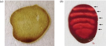
Contact line deposits for drops dried on a vertical surface for (a) coffee and (b) an aqueous solution of ferroin. The upper contact line depins in both cases. The differences in the deposits is due to re-pinning of the contact line multiple times in (b) and not at all in (a). The arrows in (b) indicate separate deposition bands formed each time the contact line is pinned. The direction of gravity is from top to bottom.

Drops dried on vertical surfaces typically leave a residue, like the one shown in figure 1(a), that is larger downslope. While this result may seem natural given that gravity acts downward, it is at odds with the existing theory of contact line deposits. As argued by Deegan et al. (Reference Deegan, Bakajin, Dupont, Huber, Nagel and Witten1997), at early times the mass of the deposit
 $m$
grows with time
 $t$
as
 $t^{{\it\zeta}}$
, where
 ${\it\zeta}$
is a function of the local contact angle
 ${\it\alpha}$
. For an almost flat drop,
 ${\it\alpha}\simeq 0$
and
 ${\it\zeta}\rightarrow 4/3$
; for
 ${\it\alpha}={\rm\pi}/4$
,
 ${\it\zeta}=1/3$
; and for a hemispherical drop
 ${\it\alpha}={\rm\pi}/2$
,
 ${\it\zeta}=0$
. In short, bigger contact angles equal smaller deposition rates. When a drop is placed on an incline, the lower angle is largest and thus the theory predicts a greater upslope deposit.
Why then does the deposit in figure 1(a) so obviously differ from the theoretical prediction? Several possibilities suggest themselves immediately. If the late-time behaviour is crucial, the asymptotic theory for early times is not applicable. Even within the asymptotic theory there is a crossover time that in principle could be shorter than the drying time, leading to a later downslope deposit. The answer is more mundane and is revealed by the figure 1(b). As the drop dries the upper contact angle decreases and ultimately reaches a depinning threshold (see for example de Gennes Reference de Gennes1985). Thereafter, the lower contact line deposit remains wetted and continues to grow whereas the upper deposit is frozen at the size it had when the contact line depinned. The depinned contact line will continue to lay down deposits but at a location that depends on the vagaries of the stick–slip motion (Adachi, Dimitrov & Nagayama Reference Adachi, Dimitrov and Nagayama1995; Deegan Reference Deegan2000; Kusumaatmaja & Yeomans Reference Kusumaatmaja and Yeomans2007; Orejon, Sefiane & Shanahan Reference Orejon, Sefiane and Shanahan2011; Snoeijer & Andreotti Reference Snoeijer and Andreotti2013; Stauber et al. Reference Stauber, Wilson, Duffy and Sefiane2014).
While examples such as those in figure 1 demonstrate that larger downslopes occur, they do not rule out the possibility of larger upslope deposits. Moreover, the asymptotic theory suggests that larger upslope deposits are at least conceivable. The upslope deposit grows faster due to the evaporative singularity, but not for as long because of depinning. Nonetheless, this deposit will be larger if conditions are such that the early lead it enjoys is insuperable by the deposition that takes place downslope subsequent to the depinning event.
To investigate this possibility we numerically integrate a Lagrangian creeping flow model of a two-dimensional drop (i.e. a strip-like drop). The shape of the drop is assumed to be instantaneously in static equilibrium. The flow is generated by evaporation that we assume is diffusion limited. The evaporation rate is obtained from the exterior diffusion problem using a boundary element method. The solute is treated as passive tracers in the flow. The depinning event that terminates deposition at the upper contact line is crucial and is modelled using a receding contact angle of zero. For sufficiently large drop our model produces a larger upslope deposit.
2. Model
In order to systematically study the effect of substrate inclination on contact line deposits, we performed numerical calculations of the deposition from two-dimensional drops (i.e. strips) subject to diffusion-limited evaporations. Numerical simulations appear to be the only theoretical avenue for attacking this problem given that the shape of the drop can differ substantially from the spherical cap approximation used in previous studies. We limit the simulations to two dimensions because the full three-dimensional problem lacks any simplifying symmetry and as such is a major undertaking. Moreover, for the two-dimensional problem there is a simple exact closed-form solution for the evaporation profile of a spherical cap that we use to validate our computations.
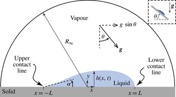
Computational domain. We model a two-dimensional sessile drop (equivalent to an infinitely long strip of fluid extending out of the paper) on a solid substrate inclined by
 ${\it\theta}$
. The upper contact angle is denoted by
 ${\it\alpha}$
. The vector labelled
 $\boldsymbol{g}$
indicates the direction of gravity. The upper right corner inset shows the physical arrangement of the substrate.

We follow the formulation of the problem used by Deegan (Reference Deegan2000). We define the depth-averaged velocity of the liquid
 $u(x,t)$
within an evaporating drop at position
 $x$
along the substrate (see figure 2 for geometry) and time
 $t$
:
 $$\begin{eqnarray}u(x,t)\equiv \frac{1}{h}\int _{0}^{h(x,t)}U(x,y,t)\,\text{d}y,\end{eqnarray}$$
where
 $y$
is the vertical distance above the substrate and
 $U$
is local velocity. Mass conservation provides the relationship between
 $u$
, the height of the interface above the substrate
 $h$
, and the flux through the interface due to evaporation
 $j$
:
 $$\begin{eqnarray}\frac{\partial h}{\partial t}=-\frac{1}{{\it\rho}}j\sqrt{1+(h^{\prime })^{2}}-\frac{\partial }{\partial x}(hu),\end{eqnarray}$$
where
 $h^{\prime }\equiv \partial h/\partial x$
, and
 ${\it\rho}$
is the density of the liquid. Integrating (2.2) from an arbitrary starting point
 $x$
to the contact line at
 $x=L$
, yields
 $u$
in terms of
 $h$
and
 $J$
:
 $$\begin{eqnarray}u(x,t)=\frac{1}{h}\int _{x}^{L}\left[\frac{1}{{\it\rho}}J\sqrt{1+(h^{\prime })^{2}}+\frac{\partial h}{\partial t}\right]\text{d}x.\end{eqnarray}$$
In general
 $h$
is coupled to the flow through the pressure and so must be solved for simultaneously with the flow field. If the evaporation rate is sufficiently slow, however, the interface assumes the equilibrium shape prescribed by the Young–Laplace equation
 $$\begin{eqnarray}{\it\gamma}\left[\frac{h^{\prime \prime }}{(1+h^{\prime })^{3/2}}\right]-{\it\rho}\boldsymbol{g}(x\sin {\it\theta}-h\cos {\it\theta})=P,\end{eqnarray}$$
with the boundary conditions fixed by the conditions that the contact line is pinned at
 $x=\pm L$
and the upper contact angle
 ${\it\alpha}$
is fixed:
 $$\begin{eqnarray}\displaystyle \left.\begin{array}{@{}c@{}}h(x=\pm L,t)=0,\\ h^{\prime }(x=-L,t)={\it\alpha}(t).\end{array}\right\} & & \displaystyle\end{eqnarray}$$
Here
 ${\it\gamma}$
is the liquid–air surface tension,
 ${\it\theta}$
is the inclination of the substrate relative to the direction of gravity,
 $\boldsymbol{g}$
is the acceleration due to gravity, and
 $P$
is an unknown coefficient determined by the boundary conditions. Note that specifying the contact angle is equivalent to specifying the volume.
Given the interface shape, the evaporation rate in the diffusion-limited regime is determined by the diffusion equation for the vapour field above the drop. With the assumption that the vapour density
 $c$
is close to steady state, the time dependence vanishes and the density obeys Laplace’s equation. The boundary conditions follow from the physical conditions that the atmosphere immediately outside the drop is saturated with vapour, on the solid substrate the vapour flux vanishes, and far from the drop the density approaches the prevailing density
 $c_{\infty }$
:
 $$\begin{eqnarray}\displaystyle \left.\begin{array}{@{}c@{}}{\rm\nabla}^{2}c=0,\\ \partial _{y}c=0\quad \text{on substrate},\\ c=c_{s}\quad \text{on surface of drop},\\ c=c_{\infty }\quad \text{as }R\rightarrow R_{\infty },\end{array}\right\} & & \displaystyle\end{eqnarray}$$
where
 $c_{s}$
is the saturated vapour density. Given
 $c(x,t)$
, the flux at the surface follows from
 $j=-D\boldsymbol{n}\boldsymbol{\cdot }\boldsymbol{{\rm\nabla}}c$
, where
 $D$
is the diffusion coefficient for vapour.
We treat the solute as a passive tracer, an assumption shown to be quantitatively accurate for dilute (<1 %) suspensions (Deegan et al.
Reference Deegan, Bakajin, Dupont, Huber, Nagel and Witten2000). The amount of solute advected to the contact line is specified by
 $u$
. Consider a packet of fluid initially at
 $x(0)=x_{o}$
. Under the action of the flow, the packet is transported towards the contact line and ultimately reaches the contact line at some time
 $T(x_{o})$
. But within this time all the fluid that initially lies between
 $x_{o}$
and the contact line will also have reached the contact line. Hence, the mass at the contact line
 $m$
at
 $t=T(x_{o})$
is all the mass of solute initially between
 $x_{o}$
and the contact line:
 $$\begin{eqnarray}m_{\pm }(t)=\int _{x_{o}=T^{-1}(t)}^{\pm L}{\it\phi}h(x,t=0)\,\text{d}x,\end{eqnarray}$$
where
 ${\it\phi}$
is the initial concentration of non-volatile solute in the drop, and the ± is for the upper (+) and lower (−) contact lines. The relationship
 $T(x_{o})$
is found from
 $$\begin{eqnarray}\frac{\text{d}x}{\text{d}t}=u.\end{eqnarray}$$
This equation generates a family of curves
 $x(t;x_{o})$
parametrized by the initial position
 $x_{o}$
. By integrating
 $x$
forward in time, the time at which
 $x$
reaches one of the contact lines is
 $T(x_{o})$
.
3. Numerical scheme
The model was rendered dimensionless by rescaling lengths by
 $\ell =\sqrt{{\it\gamma}/{\it\rho}\boldsymbol{g}}$
, vapour concentrations by
 $c_{s}-c_{\infty }$
, times by
 $(c_{s}-c_{\infty })/(\ell ^{2}D{\it\rho})$
, and masses by
 ${\it\phi}\ell ^{2}$
. This yields a single dimensionless parameter, the Bond number
 $\mathit{Bo}={\it\rho}\boldsymbol{g}L^{2}/{\it\gamma}=(L/\ell )^{2}$
, which determines the influence of gravity. Since the contact angle
 ${\it\alpha}$
decreases monotonically in time, the contact angle was used as the independent variable,
 $$\begin{eqnarray}\frac{\text{d}}{\text{d}{\it\alpha}}\left[\begin{array}{@{}c@{}}x\\ t\end{array}\right]=\frac{1}{\dot{{\it\alpha}}}\left[\begin{array}{@{}c@{}}u\\ 1\end{array}\right],\end{eqnarray}$$
where
 $$\begin{eqnarray}u(x,{\it\alpha})=\frac{1}{h(x,{\it\alpha})}\left(\int _{0}^{s(x)}j(s,{\it\alpha})\,\text{d}s+\dot{{\it\alpha}}\int _{-L}^{x}\frac{\partial }{\partial {\it\alpha}}h(x,{\it\alpha})\,\text{d}x\right),\end{eqnarray}$$
and
 $s$
is the arclength along the drop surface from
 $x=-L$
. Starting from the initial condition
 ${\it\alpha}={\it\alpha}_{o}$
, on each iteration
 ${\it\alpha}$
was decremented with a variable step size. For the
 $\imath$
th iteration:
-
(i) The position of the drop’s surface above the substrate
 $h_{ij}\equiv h({\it\alpha}_{i},x_{j})$
was calculated from (2.4) using a finite difference Matlab routine BVP4c. We used 1280 nodes uniformly spaced on the
$x$
-axis.
-
(ii) The evaporation flux
$j_{i}$
(spatial dependence suppressed) was calculated from (2.6) by the boundary integral method (Ang Reference Ang2008) using the result of step (i) to complete the specification of the domain. In all cases,
$R_{\infty }=10L$
. The surface of the drop was meshed with the 1280 nodes
$(x_{j},h_{ij})$
obtained from the Young–Laplace equation. -
(iii) The shape was recomputed for
$1.01{\it\alpha}_{i}$
to obtain
$\partial h_{i}/\partial {\it\alpha}$
. -
(iv) We compute
$\dot{{\it\alpha}}$
from the ratio
$-\int _{0}^{s(L)}\,\text{d}s\;j_{i}/\!\int _{-L}^{L}\,\text{d}x\;\partial h_{i}/\partial {\it\alpha}$
. -
(v) We compute
$u$
from the above values inserted into (3.2). -
(vi) Equation (3.1) was integrated with the forward Euler method.




The result of the above procedure was a family of curves
 $x(t;x_{o})$
, from which the resulting mass of the solute deposit was computed using (2.7).
4. Validation
When the substrate is horizontal and the size of the drop is small compared to the capillary length, the drop takes the form of a circular cap. For these conditions Yarin et al. (Reference Yarin, Szczech, Megaridis, Zhang and Gamota2006) found an exact analytical expression for the evaporation flux for a strip-like droplet. Near the contact line this expression is approximated by
 $$\begin{eqnarray}j=\frac{Dc_{s}}{L}\left[\frac{1-{\it\lambda}}{\ln (R_{\infty }/L)-\ln (1-{\it\lambda})}\right]\left(\frac{2L}{s}\right)^{{\it\lambda}},\end{eqnarray}$$
where
 $s$
is the distance along the drop surface from the contact line, and
 ${\it\lambda}=({\rm\pi}-2{\it\alpha})/$
 $(2{\rm\pi}-2{\it\alpha})$
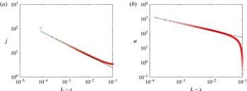
. Figure 3(a) shows a comparison of
 $j$
calculated from the analytical expression and the boundary element code for a small Bond number. The agreement is good down to 10−4.
Validation of numerical simulations with the analytical result for a circular drop with
 $\mathit{Bo}=0.01$
,
 ${\it\alpha}=5^{\circ }$
, and
 ${\it\theta}=0$
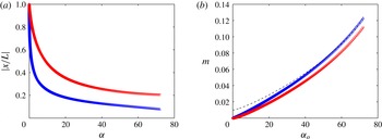
. (a) Evaporation flux (mass per unit time per unit length); (b) velocity versus distance from the contact line. Red circles, simulations; dashed green line, analytical result from Yarin et al. (Reference Yarin, Szczech, Megaridis, Zhang and Gamota2006); solid black line, asymptotic results in (4.1). All units are dimensionless.

We can also use the prefactors provided by (4.1) to calculate early-time asymptotic results for the depth-averaged velocity and the mass at the contact line. Within a horizontal distance
 ${\it\epsilon}\ll 1$
,
 $$\begin{eqnarray}\displaystyle h & {\sim} & \displaystyle {\it\epsilon}\tan {\it\alpha},\end{eqnarray}$$
 $$\begin{eqnarray}\displaystyle s & {\sim} & \displaystyle {\it\epsilon}\sec {\it\alpha},\end{eqnarray}$$
 $$\begin{eqnarray}\displaystyle J & = & \displaystyle As^{-{\it\lambda}}\sim A(\cos {\it\alpha})^{{\it\lambda}}{\it\epsilon}^{-{\it\lambda}},\end{eqnarray}$$
 $A$
is a constant fixed by the geometry of the drop. Integrating (2.3) with these expressions yields
 $$\begin{eqnarray}u\sim \frac{A}{{\it\rho}}\frac{(\cos {\it\alpha})^{{\it\lambda}}}{(1-{\it\lambda})\sin {\it\alpha}}{\it\epsilon}^{-{\it\lambda}}\equiv B{\it\epsilon}^{-{\it\lambda}}.\end{eqnarray}$$
By integration of
 $u=-\text{d}{\it\epsilon}/\text{d}t$
, the relationship between the starting position
 ${\it\epsilon}$
and the transit time to the contact line is
 $$\begin{eqnarray}{\it\epsilon}\sim [({\it\lambda}+1)Bt]^{1/({\it\lambda}+1)}.\end{eqnarray}$$
Combining this with (2.7) yields
 $$\begin{eqnarray}m\sim {\textstyle \frac{1}{2}}{\it\phi}\tan {\it\alpha}{\it\epsilon}^{2}\sim {\textstyle \frac{1}{2}}{\it\phi}\tan {\it\alpha}[({\it\lambda}+1)Bt]^{{\it\zeta}},\end{eqnarray}$$
where
 $$\begin{eqnarray}{\it\zeta}=\frac{2}{{\it\lambda}+1}=\frac{{\rm\pi}-{\it\alpha}}{{\textstyle \frac{3}{4}}{\rm\pi}-{\it\alpha}}.\end{eqnarray}$$
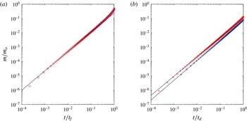
Figures 3(b) and 4(a) compare (4.5), (4.7) and results from our numerical calculation. The agreement between the numerics and the asymptotic expressions is very good within the limitations of the latter (i.e. early times and short distances from the contact line).
(a) Mass deposited on upper (red ○) and lower (blue ●) contact lines for a flat substrate
 $({\it\theta}=0),\mathit{Bo}=1$
and
 ${\it\alpha}_{o}=5^{\circ }$
, normalized to the total mass of solute in the drop
 $m_{o}={\it\phi}\int _{-L}^{+L}h(x,0)\,\text{d}x$
versus time normalized to the drying time
 $t_{f}$
. (b) Normalized mass deposited on the upper (red ▵) and lower (blue ▿) contact line for
 $\mathit{Bo}=1$
,
 ${\it\alpha}=5^{\circ }$
, and
 ${\it\theta}=40^{\circ }$
versus time normalized by the time at which the upper contact line depins
 $t_{d}$
. The initial time for data in (b) are different because of the different speed of the Lagrangian elements used to track the mass. The solid lines are the early-time asymptotic results. All units are dimensionless.

5. Results
Figure 4 shows typical results from our simulations. The upper contact line deposit is greater at all times right up to and including the depinning point (i.e.
 ${\it\alpha}=0$
). This result is in agreement with the early-time asymptotics. For
 $t\ll 1$
the mass deposited at the upper and lower contact lines,
 $m_{u}$
and
 $m_{d}$
, is of order
 $t^{{\it\zeta}_{u}}$
and
 $t^{{\it\zeta}_{d}}$
, respectively. Since the upper contact angle is smaller than the lower contact angle,
 ${\it\zeta}_{u}<{\it\zeta}_{d}$
and
 $m_{d}\ll m_{u}$
as
 $t\rightarrow 0$
.
Figure 4 also shows that even outside the asymptotic regime the upper deposit is greater. This was the case for all initial conditions and system parameters we examined. Since
 $m_{d}\gg m_{u}$
as
 $t\rightarrow \infty$
, there exists a crossover time where
 $m_{d}$
and
 $m_{u}$
exchange dominance. Our simulations imply that the crossover time is always longer than the depinning time. We have no a priori reason to expect this; nonetheless, it is so.
(a) Normalized distance from the centre of two fluid elements that simultaneously reach the contact line at the moment of depinning (i.e.
 ${\it\alpha}=0$
), versus upper contact angle for
 $\mathit{Bo}=0.25$
and
 ${\it\theta}=47^{\circ }$
. The contact angle is a parametrization of time, and so larger contact angles equal earlier times. The red ▿ (blue ▵) correspond to an element advected towards the lower (upper) contact line. (b) Mass deposited at the contact line at the moment of depinning as a function of the initial upper contact angle. Colours and symbols as in (a). The dashed black line corresponds to mass at the lower contact line shifted upwards by the mass of solute remaining in the drop at the depinning moment. The point at which the dashed black line crosses the curve of blue ▵ indicates the minimum initial contact angle needed to ensure that the upper contact line has a greater deposit. After the upper contact line depins, the remaining mass will continue to be deposited at both contact lines, but because the upper one is mobile the deposit will be smeared out.

Following depinning, the upper deposit experiences no further growth, whereas the lower deposit continues to grow. Modelling the process beyond this point would be of limited utility without focusing on a particular solute size and shape, and liquid–substrate wettability because the results depend sensitively on these factors. Instead, we answer the question of whether it is possible that the upper deposit is greater than the lower deposit for a particular depinning criterion,
 ${\it\alpha}=0$
. This criterion demands some justification. For pure fluids, the natural choice for
 ${\it\alpha}$
would be the so-called ‘receding contact angle’. However, in ring-forming drops the depinning angle is found experimentally to be far lower and often close to zero. Deegan (Reference Deegan2000) ascribed this anomalously low receding contact angle as a self-pinning effect caused by alterations of the substrate geometry due to the accumulation of solute.
We calculated the deposition mass at both contact lines up to the point that
 ${\it\alpha}=0$
. Thereafter, we assume that all the remaining solute is ultimately swept to the lower contact line, the most favourable scenario for a larger lower deposit. Rather than calculating the deposit for each initial condition, we use a scheme that captures all initial conditions (
 ${\it\alpha}_{o}$
) in a single calculation. Consider the element of fluid that arrives simultaneously at the upper and lower contact line at the moment of depinning. These elements lie somewhere in the bulk at earlier times; figure 5(a) illustrates a particular set of positions
 $x_{u}$
and
 $x_{d}$
for
 $\mathit{Bo}=0.25$
and
 ${\it\theta}=47^{\circ }$
. Any initial contact angle is captured by these trajectories and completely prescribes the mass that will be deposited at the contact line between
 $t=0$
and the depinning time. For example, for an initial contact angle
 ${\it\alpha}_{o}=20^{\circ }$
:
 $x_{d}=0.36L$
and
 $x_{u}=-0.2L$
, and
 $m_{d}=\int _{0.36L}^{L}\,\text{d}x\;h|_{{\it\alpha}={\it\alpha}_{o}}$
and
 $m_{u}=\int _{-L}^{-0.2L}\,\text{d}x\;h|_{{\it\alpha}={\it\alpha}_{o}}$
. Figure 5(b) shows the mass at each contact line at the moment of depinning versus the initial contact angle. It also shows (dashed black line) how we compute the initial contact angle needed for the upper deposit to be larger.
For droplets much smaller than the capillary length, gravity does not affect the shape of the drop and therefore at any inclination the upper and lower deposits are identical. For droplets that are 2–3 times larger than the capillary length, the droplet cannot be pinned except at the smallest of inclinations. Thus, the interesting range is
 $0.01<\mathit{Bo}<4$
.
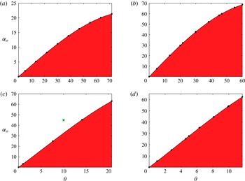
The results of our calculations, summarized in figure 6 for various
 $\mathit{Bo}$
, show that for any inclination there are two regimes: (i) for large initial contact angles even if all the remaining solute is swept into the lower contact line, the upper contact line will have a larger deposit; and (ii) for small initial contact angles assuming that all the remaining solute is swept to the lower contact line, the lower contact line will have a larger deposit.
Phase diagram as a function of initial contact angle
 ${\it\alpha}_{o}\equiv {\it\alpha}(0)$
and inclination of the substrate
 ${\it\theta}$
for various values of
 $\mathit{Bo}$
: (a) 0.0625, (b) 0.25, (c) 0.56, (d) 1.0. White indicates a larger deposit at the upper contact line, while red indicates a larger deposit at the lower contact line. The green
 $\bigstar$
corresponds to the parameters of the deposition pattern in figure 7.

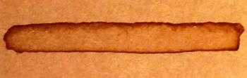
We carried out qualitative experiments to test our main computational prediction: that there exist certain configurations that produce bigger upslope deposits. We made two-dimensional drops by placing a strip of coffee on a highly corrugated substrate. We tilted the substrate, and observed the resulting deposition. Figure 7 shows an example of the deposit for
 $\mathit{Bo}=0.5$
,
 ${\it\theta}=10^{\circ }$
, and
 ${\it\alpha}_{o}=50^{\circ }$
. Referring to figure 6, the upper contact line deposit is predicted to be larger, and the experiment is in agreement with the prediction.
Strip of coffee dried on a substrate inclined at
 ${\it\theta}=10^{\circ }$
. The drop was originally 0.4 cm wide (
 $\mathit{Bo}=0.5$
), and had an upper contact angle
 ${\it\alpha}_{o}=45^{\circ }$
and a lower contact angle of 49°. The component of gravity tangent to substrate points from top to bottom in the image. Note that the deposit at the upper contact line is larger.

6. Discussion and conclusions
We conducted numerical simulations of the formation of contact line deposits from a two-dimensional drop on an incline undergoing evaporation. We find, in agreement with the early-time asymptotics, that the upper deposit grows faster. However, the upper contact line eventually depins and thereafter there is no further growth of the upper deposit. In contrast, the lower contact line always remains pinned and will continue to grow after the upper line depins. Whether the upper deposit is greater than the lower one or vice versa depends on the difference in their respective masses at the moment of depinning, which in turn, as shown in figure 6, depends on the initial volume of the drop and inclination of the substrate. A larger initial volume delays depinning and thus favours a larger upper deposit. A greater inclination promotes depinning but also a more rapid/slower growth of the upper/lower deposit; thus, its effects are indeterminate.
Our criterion for depinning (i.e. the receding contact is zero degrees) is somewhat simplistic, particularly when compared with the state of the art (e.g. Rio et al. Reference Rio, Daerr, Lequeux and Limat2006; Musterd et al. Reference Musterd, van Steijn, Kleijn and Kreutzer2014). However, it is known that contact line deposition pins the contact line far more robustly than the simpler case of pure fluid on a chemically or microscopically rough substrate due to self-pinning: the roughening of the substrate that occurs as the deposit accumulates reinforces whatever defects pinned the contact line in the first place (Deegan Reference Deegan2000). Even in the cases when all the system parameters are specified, modelling the motion of the contact line in the presence of ring formation has met with limited success. Thus, in lieu of a more complicated model that would be suspect anyway, we chose the simpler criterion used above.
The simulations presented above were for two-dimensional drops, i.e. long strips of fluids. While drops are usually roughly circular, computing the deposition for this more realistic case is a daunting task given that the direction of the velocity field within the drop is likely to vary with depth and thus entail full three-dimensional computations (three space plus one time), rather than the simpler one space plus one time employed. Nonetheless, we can extrapolate to the circular case from our results. Depinning of the upper contact line will be more difficult since the contact angle will vary smoothly along the perimeter, i.e. even if the contact angle reaches zero at one point, the adjacent segments of the contact line will be able to maintain some tension on the line. However, we do not expect any qualitatively significant deviation from our main conclusion: there will exist combinations of inclination and initial volume that can yield either of the cases of enhanced lower or upper deposits.
This work was motivated by the need to determine a posteriori if a drop had dried on a flat or vertical surface in a forensic investigation. Our results show that it is difficult to reconstruct the inclination of the substrate based solely on the shape of the deposit because a slightly larger or smaller initial drop volume could change the ratio of masses. It may be possible to carry out the reconstruction based on the stick–slip pattern left by the deposit as in figure 1(b), but as demonstrated in figure 1(a) this stick–slip motion is not always present.
Acknowledgements
The authors thank the James S. McDonnell Foundation for support through a 21st Century Science Initiative in Studying Complex Systems Research Award, and the National Science Foundation for support under grant 0932600. R.D.D. thanks the Lady Davis Foundation for support.