Effects of thermophoresis on high-pressure binary-species boundary layers with uniform and non-uniform compositions

Takahiko Toki; Josette Bellan

doi:10.1017/jfm.2022.923

Effects of thermophoresis on high-pressure binary-species boundary layers with uniform and non-uniform compositions

Published online by Cambridge University Press: 01 December 2022

Takahiko Toki

and

Josette Bellan

Show author details

Takahiko Toki: Affiliation:
California Institute of Technology, Pasadena, CA 91125, USA
Josette Bellan*: Affiliation:
California Institute of Technology, Pasadena, CA 91125, USAJet Propulsion Laboratory, California Institute of Technology, Pasadena, CA 91109, USA
*: †Email address for correspondence: josette.bellan@jpl.nasa.gov

Article contents

Abstract
Introduction
Configuration, boundary conditions and initial conditions
Results
Conclusions
Funding
Declaration of interests
References

Rights & Permissions

Abstract

Direct numerical simulations of high-pressure binary-species temporal boundary layers are performed to investigate the flow physics for three situations: (1) uniform and equal composition, (2) uniform but unequal compositions and (3) non-uniform composition. Both colder- and hotter-wall situations compared with the free stream are simulated. The working fluid is a nitrogen/methane mixture. The analysis is performed at a case-specific self-similar state. Even when the initial composition is uniform, the methane mean mass fraction decreases near the colder wall, whereas it increases near the hotter wall and the mass fraction fluctuates in the entire boundary layer. Analysis of the species-mass diffusion balance and flow structures reveal that both mass-fraction variation and fluctuations are induced by the Soret effect. When the initial composition is non-uniform and the wall is colder, the methane mean mass fraction monotonically increases from the wall akin to its initial profile. However, when the wall is hotter the mean mass fraction decreases near the wall in contrast to its initial profile, a fact traced through the species-mass diffusion balance to the Soret effect being large and enriching methane near the wall. In contrast, the direction of the Soret flux is opposite for the colder wall, thus keeping the methane concentration small. Although the initial magnitude of the difference between the wall and free-stream temperature is the same in all cases, the situation is not symmetric between colder- and hotter-wall cases; the flow structure exhibits much smaller scales when the wall is hotter than when the wall is colder.

JFM classification

Boundary Layers: Boundary layer structure Mass Transport: Coupled diffusion and flow Mixing: Turbulent mixing

Information

Type: JFM Papers
Information: Journal of Fluid Mechanics , Volume 952 , 10 December 2022, A37
DOI: https://doi.org/10.1017/jfm.2022.923 [Opens in a new window]
Copyright: © California Institute of Technology, 2022. Published by Cambridge University Press

1. Introduction

Thermophoretic effects, also called Soret effects, were known as early as the 1930s and experiments describing mixture separation obtained as a result of a temperature gradient indicated the interesting potential of this technique. Using thermophoresis, Clusius & Dickel (Reference Clusius and Dickel1938) successfully separated several gaseous mixtures involving concentrations of HCl and Ne. A vast set of experimental data showing the separation of mixtures is discussed in Jones & Furry (Reference Jones and Furry1946). In an early study, Liu (Reference Liu1959) presented a two-dimensional (2D) model and steady-state approximate solution describing the separation of species in an air/H$_{2}$ or air/He boundary layer. Furthermore, Garcia-Ybarra & Castillo (Reference Garcia-Ybarra and Castillo1997) reported and modelled thermophoresis in atmospheric-pressure laminar boundary layers using a 2D model and derived asymptotic solutions. The Soret effect was also described in detail by Saghir et al. (Reference Saghir, Jiang, Chacha, Yan, Khawaja and Pan2005) who showed its existence for methanol–water and ethanol–water mixtures (10 % mass fraction of water in each case) at 1 bar and for methane (20 % molar fraction)–n-butane (80 % molar fraction) near the critical point. The modification of hydrocarbon transport in compressed non-isothermal gases as a result of thermophoresis was addressed by Rosner & Arias-Zugasti (Reference Rosner and Arias-Zugasti2007). In the context of flames, thermophoresis has mainly been discussed with respect to hydrogen–air flames (Grcar, Bell & Day Reference Grcar, Bell and Day2009; Yang et al. Reference Yang, Law, Sung and Zhang2010) and spray flames (Ben Dakhlia, Giovangigli & Rosner Reference Ben Dakhlia, Giovangigli and Rosner2002). Thus, there is ample evidence that thermophoresis induces species separation in a mixture of chemical species.

A situation in which thermophoresis is pertinent is that occurring in many propulsion systems such as diesel engines, gas turbine engines and rocket engines, where the wall of the combustion chamber is exposed to a flow containing many species. In those engines, the pressure is above critical pressures for several species of the mixture, and sometimes it may even be above the critical pressure for the fluid species mixture, thus making the study of high-pressure multi-species turbulent boundary layers a topic of wide interest. Thermophoresis can also become significant in cooling pipes (i.e. channels) of those engines as fuel is also used in aircraft as a convenient heat sink. Indeed, in aircraft, fuel combustion provides the energy and power to propel the aircraft; however, the fuel dispenses more energy than is used for propulsion purposes. Some of the heat released is transformed into useful power; however, the remaining heat must be dissipated or absorbed by other processes, so that it is not destructive to the engine. In a typical aircraft, approximately half of the heat is exhausted, and the other half must be appropriately mitigated so that it does not damage the aircraft structural components. As fuel is a liquid with good heat transfer properties, using it as a cooling agent is convenient because a large quantity of fuel is available and must be carried on the aircraft for operation purposes. Heating fuel prior to it entering the engine combustor is advantageous to the engine efficiency, but thermal stability of conventional jet fuel provides some limits. If fuel thermal limits are exceeded, it can degrade by oxidising reactions or pyrolysis. As a result, viscous deposits can form in the fuel lines. Such deposits can foul the heat-transfer surfaces, leading to decreased heat-transfer performance and/or decreased engine performance (Faith, Ackerman & Henderson Reference Faith, Ackerman and Henderson1971). Controlling the composition of the fluid in contact with surfaces is very desirable as it has the potential of eliminating the harmful surface reactions. Control and optimisation of this cooling process is still an active topic of research and success in this endeavor could affect both military and commercial aircraft performance and address pipe wall durability. The present study is motivated by this intriguing possibility and the desire is to understand the physics that may lead to such control rather than address the practical situation.

Owing to the high temperature difference between wall and fluid, the high-pressure multi-species turbulent boundary layer in the above-described situation is the site of large temperature gradients in the wall-normal direction. What makes the study of these boundary layers different from the typical investigations involving a single chemical species (Kawai Reference Kawai2019) is that, as recently explained by Toki & Bellan (Reference Toki and Bellan2021) for a colder-than-fluid wall situation, the Soret effect, which becomes more prominent at high pressures, plays a significant role in determining the chemical composition at the wall, consistent with the studies (e.g. Liu Reference Liu1959; Garcia-Ybarra & Castillo Reference Garcia-Ybarra and Castillo1997) identifying such occurrences. The study of Toki & Bellan (Reference Toki and Bellan2021) used direct numerical simulations (DNS) to understand the physics in that exploratory investigation, however, no equivalent DNS study exists of the hotter-than-fluid wall despite the fact that such a large temperature gradient may significantly influence flow physics in the multi-species turbulent boundary layer at high pressure. The advantage of DNS compared with the 2D laminar boundary layer steady-state solutions of the past is (1) that the three-dimensionality of the physical situation is addressed, a fact which is particularly important for turbulent situations, (2) that the time-dependent aspect is fully addressed and (3) that all scales of the flow relevant to dissipation are computed, thereby permitting a thorough analysis of the results and the identification of relationships which would remain hidden otherwise. According to Moin & Mahesh (Reference Moin and Mahesh1998), DNS allows significant insight into turbulent physics from the study of idealised situations that cannot be easily attained in a laboratory, and thus the results from these DNS are akin to “novel numerical experiments”.

To investigate the flow physics of single-species boundary layers at high-pressure condition, several DNS have been performed and discussed in the literature. For example, Bae, Yoo & Choi (Reference Bae, Yoo and Choi2005) and Bae, Yoo & McEligot (Reference Bae, Yoo and McEligot2008) simulated heated $\text {CO}_{2}$ turbulent vertical pipe and annular flows with buoyancy effects at small Mach numbers. They discovered that buoyancy effects cause M-shaped velocity profile and the unique velocity profile induces reduction of turbulent heat fluxes. Nemati et al. (Reference Nemati, Patel, Boersma and Pecnik2015, Reference Nemati, Patel, Boersma and Pecnik2016) and Peeters et al. (Reference Peeters, Pecnik, Rohde, Hagen and Boersma2016) also simulated vertical pipe and annular flows at small Mach numbers. The results from those investigations revealed that variations in dynamic viscosity and density significantly affect turbulent statistics and turbulent structure. Wan et al. (Reference Wan, Zhao, Liu, Wang and Lei2020) extended a temperature transformation proposed by Patel, Boersma & Pecnik (Reference Patel, Boersma and Pecnik2017), and demonstrated the transformation using their DNS data of turbulent channel flow of supercritical $\mathrm {{CO_{2}}}$. While the previous studies relied on the low-Mach-number assumption, Kawai (Reference Kawai2019) simulated heated boundary layers of supercritical hydrogen over zero-pressure-gradient flat plates using a fully compressible DNS. Kawai (Reference Kawai2019) reported that real fluid effects at transcritical conditions induce strong density fluctuations and alter the Reynolds shear stress profile. Ma, Yang & Ihme (Reference Ma, Yang and Ihme2018) studied a planar turbulent channel flow of supercritical nitrogen and demonstrated that semilocal scaling is appropriate near a cooled wall, whereas the same scaling has limited success near a hot wall where violent fluctuations are found. These differences between colder-versus-hotter-than-fluid wall indicate that the physics of two situations may also be different when the fluid is a binary-species mixture. Kim, Hickey & Scalo (Reference Kim, Hickey and Scalo2019) simulated transcritical channel flow of R-134a and discussed effects of pseudophase change on turbulent dynamics. Toki, Teramoto & Okamoto (Reference Toki, Teramoto and Okamoto2020) also simulated a planar turbulent channel flow of supercritical nitrogen and introduced a temperature transformation in the logarithmic region that accounts for the temperature variations of the mean density and of the isobaric specific heat in that region. Guo, Yang & Ihme (Reference Guo, Yang and Ihme2022) performed a planar turbulent channel flow of supercritical nitrogen with increasing a density change ratio in the channel to approximately 20, and provided a framework to guide the development of models for wall-bounded transcritical turbulence.

These DNS studies have mainly focused on effects of variations in thermodynamic properties and molecular transport properties in single-species boundary layers at high-pressure conditions, whereas to the best of the authors’ knowledge there is only a single study that investigated boundary layers composed of more than one species (Toki & Bellan Reference Toki and Bellan2021). That study, which was conducted for a fluid mixture of nitrogen (N$_{2}$) and methane (CH$_{4}$) revealed that the Soret effect becomes occasionally larger in magnitude than the molecular diffusion flux near the wall. As a result, the Soret effect was found to induce uphill diffusion. To the best of the authors’ knowledge, this is the only documented situation so far in which uphill diffusion was identified for a binary-species mixture, as in an isobaric and isothermal situation it can only exist for a mixture of three or more species (Duncan & Toor Reference Duncan and Toor1962; Taylor & Krishna Reference Taylor and Krishna1993; Sciacovelli & Bellan Reference Sciacovelli and Bellan2019). In the previous study, a mass fraction gradient was imposed in the wall-normal direction and, thus, the influence of the Soret effect on a boundary layer having an initially uniform fluid mixture remains unknown, as does the Soret effect for the hotter wall than the free-stream temperature.

To fill the existing knowledge gap, the influence of the Soret effect on flow physics of binary-species boundary layers at conditions still unexplored is investigated here by performing DNS of binary-species boundary layers under high-pressure situations. The initial composition of the binary species is of three different types: (1) uniform and of equal compositions, (2) uniform but of unequal compositions or (3) non-uniform compositions. Both hotter- and colder-wall cases are simulated and the difference in outcome between these temperature conditions are highlighted. Compared with practical applications, some of which have been discussed above. The temperature gradient, $\boldsymbol {\nabla } T,$ is here selected to be modest so that the results are expected to be conservative; that is, if species separation and uphill diffusion is found in the present results, in practical applications these phenomena will be considerably more significant. Compared with previous simulations relying on simpler models, we show here that species separation is accompanied by uphill diffusion, a phenomenon never shown in the past to result from the Soret effect under the general conditions of the present simulations.

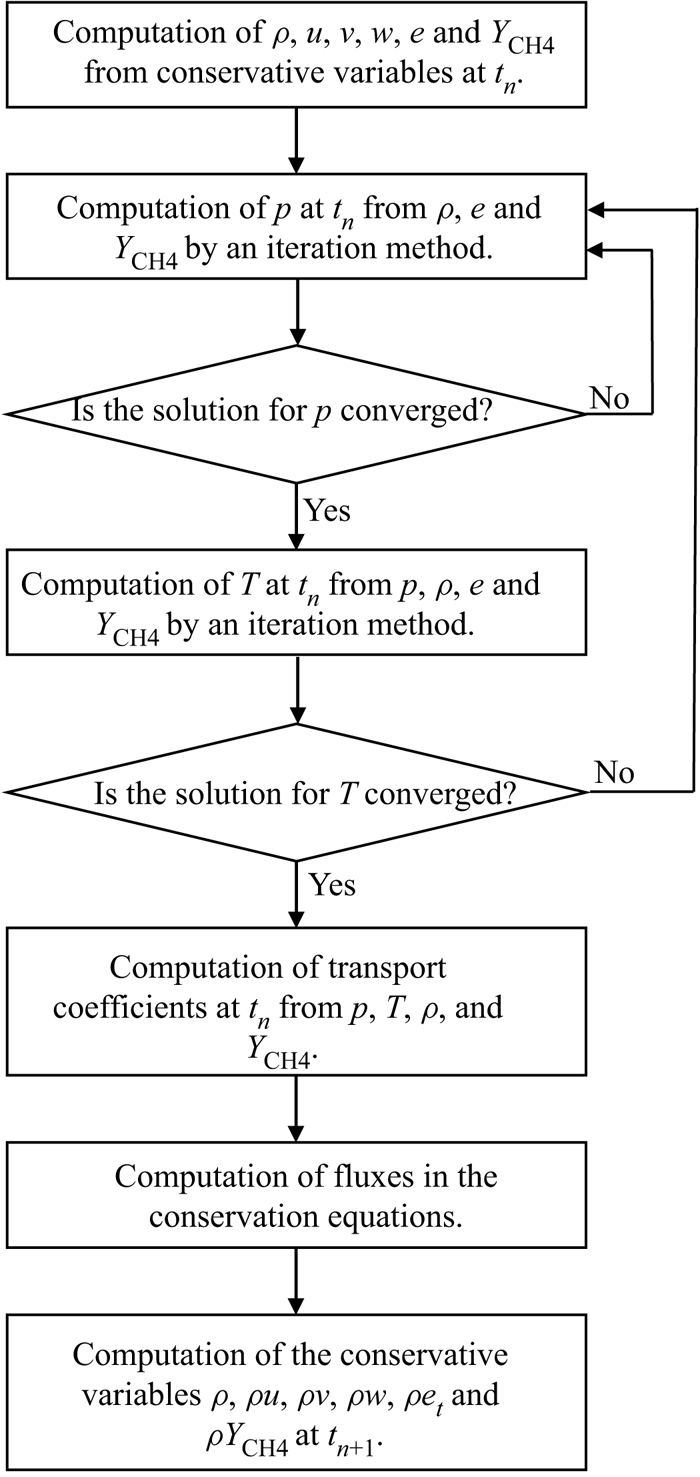
This paper is organised as follows. As the governing equations and numerical methods are the same as those in a previous study (Toki & Bellan Reference Toki and Bellan2021), they are described in Appendices A and B. The configuration, boundary conditions and initial conditions are summarised in § 2. The results are examined in § 3, and the discussion primarily addresses differences between hotter- and colder-wall cases, and between uniform and non-uniform initial mixtures. The findings from this study are summarised in § 4.

2. Configuration, boundary conditions and initial conditions

The present configuration is that of a temporal boundary layer, an approach which is justified by the realisation that temporal boundary layers and spatial boundary layers have the same physics (e.g. Martín Reference Martín2004; Kozul, Chung & Monty Reference Kozul, Chung and Monty2016). In addition, the applicability of this configuration to the high-pressure and binary-species boundary layers was already shown by Toki & Bellan (Reference Toki and Bellan2021). To be consistent with boundary layer notation in the literature, $(x_{1},x_{2},x_{3})\equiv (x, y, z)$ denote the streamwise, wall-normal and spanwise directions and $(u_{1},u_{2},u_{3})\equiv (u,v,w)$. 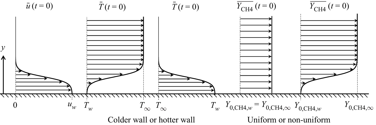Similar to the study of Toki & Bellan (Reference Toki and Bellan2021), the working fluid is a mixture of N$_{2}$ and CH$_{4}$. Figure 1 provides a sketch of the configuration. The wall moves at constant velocity, whereas the far-field is at rest. Periodic boundary conditions are applied to the streamwise ($x$) and spanwise ($z$) directions. No-slip wall conditions are applied at the wall, and the temperature and velocity are there constant in space and time. The simulation is initiated with a thin mixing layer (see § 2.1), and continues until the flow field reaches a target Reynolds number. In the past, the same configuration was used by Kozul et al. (Reference Kozul, Chung and Monty2016) to conduct DNS of an incompressible boundary layer, and it was shown that turbulent statistics of the temporal set-up agree very well with those of spatial boundary layers. In contrast to Kozul et al. (Reference Kozul, Chung and Monty2016), the upper-domain boundary condition consists of non-reflecting boundary conditions (Okong'o & Bellan Reference Okong'o and Bellan2002); the mass flux of each species is set to be null at a wall.

Figure 1.

Sketch of initial profiles of mean streamwise velocity, temperature and mass fractions.

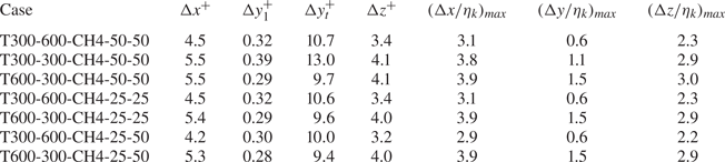
The simulations encompass three uniform and equal initial composition cases, two uniform and unequal initial composition cases and two non-uniform initial composition cases, all listed in table 1. The initial uniform composition cases are simulated to understand the approximation that would be made should a multi-species fluid be treated as a single-species fluid whereas the initially unequal composition cases represent a practical situation. The adopted notation is that subscripts $w$ and $\infty$ indicate wall and far-field locations, respectively. In table 1, $Re_{\tau }\equiv u_{\tau }\delta _{99}\rho _{w}/\mu _{w}$ is the friction Reynolds number where $\delta _{99}$ is a length which is 99 % of boundary layer thickness, $u_{\tau }\equiv \sqrt {\tau _{w}/\rho _{w}}$ where $\tau _{w}$ is the fluid shear stress at the wall and $\rho _{w}$ is the fluid density at the wall. Table 1 lists the friction Reynolds numbers at the time when the data shown in and thereafter § 3.2 are obtained. In all simulations the Mach number, $Ma$, value associated with the wall velocity $u_{w}$ is 0.4, based on the sound speed of the initial composition at the wall. Although the $Ma$ value is modest in the realm of compressible flows, due to the strong nonlinearity of the EOS, the flow cannot be considered incompressible. Indeed, for a real-gas EOS, pressure gradients are much larger than in atmospheric flows at otherwise same conditions because small spatial changes in temperature and composition induce large changes in pressure as a result of the strong nonlinearity. The wall temperature $T_{w}$ and free-stream temperature $T_{\infty }$ are either 300 K or 600 K in all cases; the value of $T_{w}$ is 300 K and the value of $T_{\infty }$ is 600 K in the colder-wall cases, and vice versa in the hotter-wall case. The temperature difference between $T_{w}$ and $T_{\infty }$ induces the Soret effect; the relatively modest $\boldsymbol {\nabla } T$ reduces in DNS the grid size requirements compared with the larger $\boldsymbol {\nabla } T$ in practical applications while concurrently representing a conservative situation in that if the Soret effect is found to induce mixture composition changes, these changes would be significantly larger in practical applications. For comparison purposes, $T_{w} = T_{\infty }= 300$ K in T-300-300-CH4-50-50. Both $Y_{0,{\text {CH}_{4}},w},$ the initial mass fraction of CH$_{4}$ at the wall, and $Y_{0,{\text {CH}_{4}},\infty },$ the initial mass fraction of CH$_{4}$ in the far-field, have the value of 0.5 in the uniform and equal composition cases, and have the value of 0.25 in the uniform and unequal initial composition cases. For the non-uniform initial composition cases, $Y_{0,{\text {CH}_{4}},w}=0.25$ and $Y_{0,{\text {CH}_{4}},\infty }=0.5$. The mass fraction of N$_{2}$ is set to satisfy mass conservation in the entire domain. The initial pressure $p_{0}$ is 60 atm, being above the critical pressures of both N$_{2}$ and CH$_{4};$ see table 2 listing the critical properties of the species and providing information regarding their thermodynamic regime at the initial conditions, where $T_{r}$ and $p_{r}$ are the reduced temperature and reduced pressure, respectively. The gradients of $T$ and $Y_{\alpha }$ induce density variations and $\rho _{\infty }/\rho _{w}$ is the density ratio between the wall fluid and the far-field fluid.

Table 1.

List of computational cases and conditions. All symbols are defined in the text.

Table 2.

Species thermodynamic critical properties, $T_c$ and $p_c$, and reduced properties, $T_r = T/T_c$ and $p_r = p/p_c$.

Here $N_{x}$, $N_{y}$ and $N_{z}$ are the number of grid points in each direction and $\mathcal {F}$ is a scaling factor defined elsewhere (Masi et al. Reference Masi, Bellan, Harstad and Okong'o2013; Sciacovelli & Bellan Reference Sciacovelli and Bellan2019) representing the scaling of the viscosity by a reference value in order to ensure that the Reynolds number value is such that DNS is feasible. Then, all transport properties are scaled by $\mathcal {F}$, in particular ensuring that the Schmidt number and Prandtl number have physical values. In the present notation $\theta _{sl}$ is the momentum thickness of the layer (discussed in § 2.1), $\alpha$ is a real number and $\alpha \theta _{sl}$ is a parameter used to derive perturbations of the initial flow; details are provided elsewhere (Toki & Bellan Reference Toki and Bellan2021).

2.1. Initial profiles

The initial profiles are composed of mean quantities upon which perturbations are imposed. The mean profiles are based on tangent hyperbolic functions, and the perturbations are analytically derived (Toki & Bellan Reference Toki and Bellan2021). The mean profiles of velocities, temperature, mass fractions and pressure are set to resemble a mixing layer as follows:

(2.1)

\begin{gather} \bar{u}(y) =u_{w}-\frac{1}{2}u_{w}\left( 1-\tanh\left[\frac{D}{2\theta_{sl}} \left(1-\frac{y}{D}\right) \right] \right) , \end{gather}

(2.2)

\begin{gather}\bar{T}(y) =T_{w}+\frac{1}{2}(T_{\infty}-T_{w}) \left( 1-\tanh\left[ \frac{D}{2\theta_{sl}}\left( 1-\frac{y}{D}\right) \right]\right), \end{gather}

(2.3)

\begin{gather}\overline{Y_{\text{CH}_{4}}}(y) =Y_{0,{\text{CH}_{4}},w}+\frac{1}{2}( Y_{0,{\text{CH}_{4}},\infty}-Y_{0,{\text{CH}_{4}},w}) \left( 1-\tanh\left[ \frac{D}{2\theta_{sl}}\left( 1-\frac{y}{D}\right) \right] \right) , \end{gather}

(2.4)

\begin{gather}\overline{Y_{\text{N}_{2}}}(y) =1-\overline{Y_{\text{CH}_{4}}}(y), \end{gather}

(2.5)

\begin{gather}p =p_{0},\quad v=0,\quad w=0, \end{gather}

where $D$ is the displacement thickness. These profiles account for the fact that unlike for single-species boundary layers, the velocity field is affected by species mixing, and thus the growth rate of perturbations is also affected by mixing. The overline $\overline {({\cdot })}$ indicates averaging in the homogeneous ($x,z)$ plane. The displacement thickness $D$ is set to $Re_{D}\equiv Du_{w}/\nu _{w}=1000$ ($\nu _{w}\equiv \mu _{w}/\rho _{w}$), consistent with Kozul et al. (Reference Kozul, Chung and Monty2016) who did a parametric study of the initial profile based on $Re_{D}$, and demonstrated that in those cases $Re_{D}=1000$ results in a natural turbulent evolution as soon as the computation was initiated. In the present study $\theta _{sl}$ is specified by stability analyses to achieve the largest growth rate for the initial perturbations (Toki & Bellan Reference Toki and Bellan2021). The numerical methods of the stability analyses yielding the perturbations are provided elsewhere (Toki & Bellan Reference Toki and Bellan2021).

2.2. Domain size and grid spacing

The domain size is determined by a specified boundary layer thickness, $\delta _{p}$. The specified target $Re_{\tau }\simeq 500$ so as to be comparable to the incompressible spatial boundary layer of Schlatter & Örlü (Reference Schlatter and Örlü2010) for which $Re_{\tau }=492;$ the very favourable comparisons between the results of Schlatter & Örlü (Reference Schlatter and Örlü2010) and Toki & Bellan (Reference Toki and Bellan2021) validated the present temporal boundary layer approach for the moderate Mach number value in the present simulations. When $Re_{\tau }=500$, $\delta _{p}\simeq 0.07$ m, which is the value adopted here. The wall-normal domain size is set to $L_{y}=3\delta _{p}$. The streamwise domain size is set to $L_{x}=2{\rm \pi} \delta _{p}$, and the spanwise domain size is set to $L_{z}={\rm \pi} \delta _{p}$. This domain size was proved to be sufficiently large to capture the main dynamic features of the flow and the wall-normal statistics (Kozul et al. Reference Kozul, Chung and Monty2016). The grid spacing is uniform in the streamwise and spanwise directions. In the wall-normal direction the grid spacing is determined by the following tangent hyperbolic function:

(2.6)

\begin{equation} y_{j}=\frac{L_{y}}{\alpha_{st}}\tanh\left[{-}1+\frac{j-1}{N_{y}-1}\tanh ^{{-}1}(\alpha_{st})\right] , \end{equation}

where $\alpha _{st}$ is a constant value, $\alpha _{st}=0.985,$ and $N_{y}$ is a number of grid points in the wall-normal direction. The wall-normal coordinates based on wall units are defined as $y^{+}\equiv yu_{\tau }/\nu _{w}$. The grid resolutions in wall units are shown in table 3. They are evaluated as ${\rm \Delta} x_{i}^{+}\equiv {\rm \Delta} x_{i}u_{\tau }/\nu _{w}$, where ${\rm \Delta} x_{i}$ is the grid spacing in the $x_{i}$ direction; ${\rm \Delta} x^{+}$ and ${\rm \Delta} z^{+}$ are grid resolutions in streamwise and spanwise directions, respectively. The wall-normal grid spacings ${\rm \Delta} y_{t}^{+}$ and ${\rm \Delta} y_{1}^{+}$ correspond to those at the top and bottom of the domain. The values of $Re_{\tau }$ at the time when the grid resolutions are computed are those listed in table 1. In addition, table 3 lists the maximum grid spacing in terms of the Kolmogorov scale $\eta _{k}$ calculated as

(2.7)

\begin{equation} \eta_{k}=\left( \frac{\left( \bar{\mu}\right)^{3}}{(\bar{\rho})^{2} \varepsilon}\right)^{1/4}, \end{equation}

where $\varepsilon \equiv \overline {\sigma _{ij}^{\prime }\partial u_{i}^{\prime }/\partial x_{j}}$ is the turbulent kinetic energy dissipation where the notation $({\cdot })^{\prime }$ indicates fluctuation from the average. In general, it is considered that $\eta$ is the smallest scale that must be resolved in DNS, however following the study of Moin & Mahesh (Reference Moin and Mahesh1998), this requirement is too drastic. Moin & Mahesh (Reference Moin and Mahesh1998) decisively showed for various configurations, including boundary layers, that it is only necessary to resolve scales $O(\eta )$, not $\eta$. According to previous DNS studies, sufficient resolution requirements are ${\rm \Delta} x<12\min \{\eta _{k},\eta _{\theta }\},{\rm \Delta} y<2\min \{\eta _{k} ,\eta _{\theta }\},{\rm \Delta} z<6\min \{\eta _{k},\eta _{\theta }\}$ where $\eta _{\theta }\equiv \eta _{k}\sqrt {1/Pr}$ is the Bachelor scale (Zonta, Marchioli & Soldati Reference Zonta, Marchioli and Soldati2012; Lee et al. Reference Lee, Jung, Sung and Zaki2013; Patel, Boersma & Pecnik Reference Patel, Boersma and Pecnik2016; Kawai Reference Kawai2019). Table 3 indicates that the present grid resolutions indeed satisfy the requirements for $\eta$. 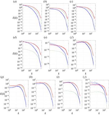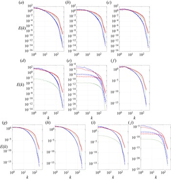As the molecular Prandtl number $Pr$ is less than 1 in all cases, the corresponding requirements for the Batchelor scale are also satisfied. For binary-species flows, these requirements may be insufficient because the Soret effect and the species mass-diffusion potentially affect the length scale of thermal diffusion (Masi et al. Reference Masi, Bellan, Harstad and Okong'o2013). Therefore, to ascertain the resolution, one-dimensional spectra of all quantities were examined (see Appendix C). These spectra reveal the smoothness typical of turbulent characteristics, and lack of energy accumulation at the smallest scales, illustrating the excellent resolution. Furthermore, to assess the selected domain size, two-point correlations were calculated (not shown) that were similar to such plots published elsewhere (e.g. Duan, Beekman & Martín Reference Duan, Beekman and Martín2010, Reference Duan, Beekman and Martín2011).

Table 3.

Grid resolution and maximum resolution normalised using the Kolmogorov scale $\eta _{k}$.

3. Results

Unlike spatial flows, temporal flows do not achieve statistical steadiness, making them unsuited to direct comparisons with experimental data; instead, temporal flows reach a self-similar state representative of the physical situation investigated. The achievement of such self-similar states is examined in § 3.1 by investigating the time-wise development of the boundary layers and the corresponding variation in important dynamic and thermodynamic quantities. Then, each case in table 1 is analysed at $Re_{\tau }\approx 500$. The uniform and non-uniform composition cases are separately addressed in §§ 3.2 and 3.3. When examining these cases, first the mean flow field and turbulent fluctuations are inspected. Second, the species-mass diffusion balance in the mean flow field is investigated with the focus on the Soret effect flux. Finally, the instantaneous flow fields are examined to discuss turbulent dynamics.

Although temporal mixing layers are not directly comparable with experimental data, as has already been noted by Kozul et al. (Reference Kozul, Chung and Monty2016) and Martín (Reference Martín2004), the physics is the same as those of spatial boundary layers that can be validated with experimental data. Adding to the credibility of the formulation described in Appendices A and B, significant portions of the present model have been validated with data, as follows: the thermodynamic model and calculations were validated with numerous data in Harstad, Miller & Bellan (Reference Harstad, Miller and Bellan1997). The calculation of the binary diffusion coefficients was validated with diverse data in Harstad & Bellan (Reference Harstad and Bellan2004b). The calculation of the pairwise diffusion coefficients that are the elements of the diffusion matrix was validated with the data of Duncan & Toor (Reference Duncan and Toor1962) in Castiglioni & Bellan (Reference Castiglioni and Bellan2018). The same DNS model and numerical method used here were also utilised in Toki & Bellan (Reference Toki and Bellan2021) in which the results were compared with those of Schlatter & Örlü (Reference Schlatter and Örlü2010) and the comparison showed coincidence of the results. Thus, the present model and code were extensively tested and validated.

3.1. Temporal evolution of the flow

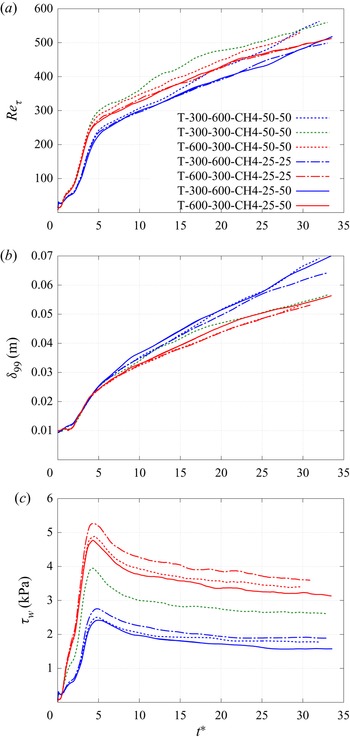
To understand the temporal evolution in the present boundary layers, figure 2 shows the time history of $Re_{\tau }$, $\delta _{99}$ and $\tau _{w}$; the computational time is scaled as $t^{\ast }\equiv tu_{w} /\delta _{p}$. The value of $Re_{\tau }$ monotonically increases and reaches the target value $Re_{\tau }=500$ between $t^{\ast }$ of 25 and 32 in all cases. Furthermore, $Re_{\tau }$ displays a steep increase before $t^{\ast }=5$ that abates past this station. The time history of $\delta _{99}$ parallels that of $Re_{\tau }$ but the difference between the slopes before and past $t^{\ast }=5$ is less dramatic. As for $\tau _{w},$ it also drastically increases with $t^{\ast }$ and reaches a peak at $t^{\ast }\simeq 5$, after which it decreases and eventually its value almost levels off. These time histories show that all profiles largely vary at the early computational time, but the slope variations at later $t^{\ast }$ become very small, a fact which is indicative of self-similarity.

Figure 2.

Time history of the development of the temporal boundary layers: (a) friction Reynolds number, (b) boundary layer thickness and (c) wall shear stress.

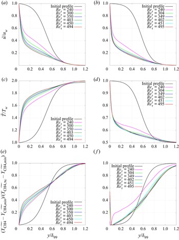
As the present simulations started with profiles inspired from mixing layer studies, it is expected that there will be a process whereby there will be a change from those initial profiles to turbulent boundary profiles. The large variations at the early computational time produce this change, and the moderate variations at the later time imply that the flow becomes a fully developed boundary layer. To investigate whether the flow fields reach those of a fully developed boundary layer, mean profiles of streamwise velocity, temperature and mass fraction of methane are compared in figure 3 for T-300-600-CH4-25-50 and T-600-300-CH4-25-50. The former case represents the colder-wall cases and the latter case represents the hotter-wall cases. To examine self-similarity in the primitive variables, the profiles are scaled by $\tilde {u}/u_{w}$, $\tilde {T}/T_{w}$ and $(\widetilde {Y_{\text {CH}_{4}}}-\widetilde {Y_{{\text {CH}_{4}},min}})/ (\widetilde {Y_{{\text {CH}_{4}},\infty }} -\widetilde {Y_{{\text {CH}_{4}},min}})$, respectively, where the subscript $min$ indicates the minimum value. The mean profiles are calculated by averaging in $(x,z)$ planes; $\widetilde {({\cdot })}$ indicates the Favre average. The comparisons show that all profiles at $Re_{\tau }=240$ are largely different from the initial profile, whereas there is good agreement in all profiles after $Re_{\tau }=400$ in both cases. This result indicates that the primitive variables fields reach self-similarity and that fully developed boundary layers are formed at $Re_{\tau }\simeq 500$. Thus, the flow fields analysed at $Re_{\tau }\simeq 500$ are at a state when the velocity, temperature and mass fraction are self-similar.

Figure 3.

Comparison of mean profiles at different computational time: (a,b) streamwise velocity, (c,d) temperature and (e,f) mass fraction of methane for cases (a,c,e) T-300-600-CH4-25-50 and (b,d,f) T-600-300-CH4-25-50.

3.2. Effects of wall versus fluid temperature at uniform binary-species initial composition

The analysis first focuses on the five cases with uniform initial composition. All analyses are conducted at $Re_{\tau }\approx 500$, as listed in table 1.

3.2.1. Mean profiles

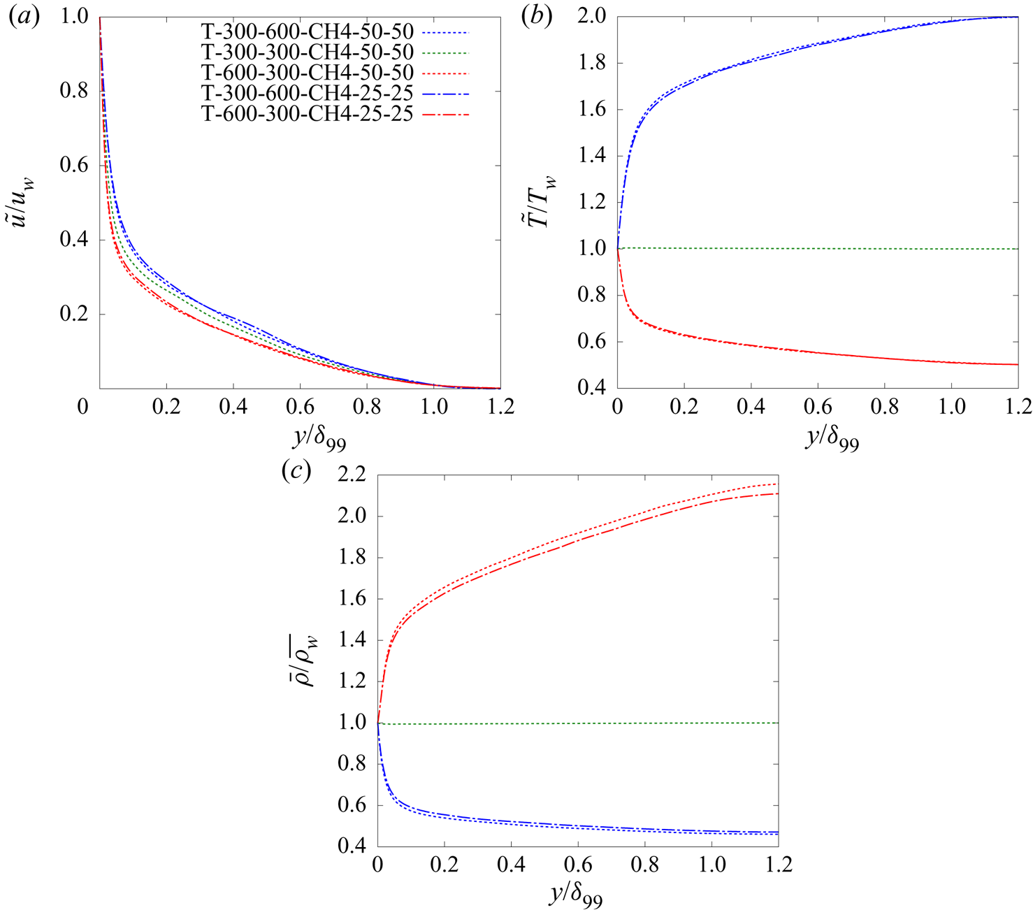
Figure 4 shows mean profiles of $\tilde {u}/u_{w}$, $\tilde {T}/T_{w}$ and $\bar {\rho }/\rho _{w}$ for the uniform initial composition cases. The mean profiles are non-dimensionalised by values at the wall. The qualitative characteristics of $\tilde {u}/u_{w}$ are the same in all cases in that the velocity monotonically decreases from the wall to the far field. The gradient of the velocity becomes large near the wall because the viscous shear stress is dominant due to the suppression of turbulence. The $\tilde {T}/T_{w}$ profile monotonically increases in cases where the wall temperature is colder than that of the free stream, and it monotonically decreases in the hotter-wall cases. In the vicinity of the wall, the temperature gradient becomes large in both the colder- and hotter-wall cases. However, $\tilde {T}/T_{w}$ is constant for T300-300-CH4-50-50, because the wall temperature is the same as that of the free stream. The $\bar {\rho }/\rho _{w}$ profiles reflect the variation in the mean temperature profiles in that there is a monotonic increase/decrease in the hotter-wall/colder-wall cases and no variation for T300-300-CH4-50-50. This comparison of the mean profiles between equal and unequal composition cases shows that all three profiles in T-300-600-CH4-50-50 agree well with those in T-300-600-CH4-25-25, and all three profiles in T-600-300-CH4-50-50 agree well with those in T-600-300-CH4-25-25. These agreements indicate that when the initial composition is uniform, the $\tilde {T}/T_{w}$ and $\bar {\rho }/\rho _{w}$ profiles are quite insensitive to the difference in initial composition.

Figure 4.

Mean profiles of (a) streamwise velocity, (b) temperature and (c) density in cases with uniform initial composition.

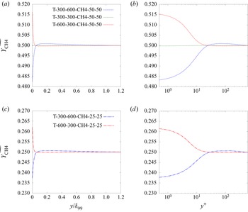
Figure 5 shows mean profiles of $\widetilde {Y_{\text {CH}_{4}}}$ as a function of either $y/\delta _{99}$ or $y^{+}$. The $\widetilde {Y_{\text {CH}_{4}}}$ is constant in T-300-300-CH4-50-50, indicating that the $\widetilde {Y_{\text {CH}_{4}}}$ does not vary from the initial composition. However, although the composition of the fluid is uniform at the initial condition, $\widetilde {Y_{\text {CH}_{4}}}$ acquires non-uniformities in the wall-normal direction in the other four cases. The non-uniformities are strong for $y^{+}\leqslant 20$, with $\widetilde {Y_{\text {CH}_{4}}}$ increasing in T-600-300-CH4-50-50 and T-600-300-CH4-25-25, representing the hotter-wall cases. In contrast, $\widetilde {Y_{\text {CH}_{4}}}$ decreases for T-300-600-CH4-50-50 and T-300-600-CH4-25-25, which are the colder-wall cases.

Figure 5.

Mean profiles of mass fraction of methane in uniform initial composition cases as a function of the outer scaling $y/\delta _{99}$ (a,c) and as a function of the wall unit $y^{+}$ (b,d) for cases (a,b) T300-600-CH4-50-50, T300-300-CH4-50-50 and T600-300-CH4-50-50 and (c,d) T300-600-CH4-25-25 and T600-300-CH4-25-25.

The relevant perspective for understanding these results involves considerations of mass diffusion. In the past, species-mass diffusion has been classified as either regular or uphill (Taylor & Krishna Reference Taylor and Krishna1993; Sciacovelli & Bellan Reference Sciacovelli and Bellan2019). Regular diffusion occurs when the flux is directed from regions of large concentrations to regions of low concentration, whereas uphill diffusion occurs when the flux is directed from regions of low concentrations to regions of large concentration. In the present situation, if only regular diffusion would occur, the mass fraction would be invariant form the initial condition which is specified as a uniform composition. Thus, the variation in the mass fraction near the wall indicates that uphill diffusion occurs in the present simulations. In addition, no variation in mass fraction only occurs for T-300-300-CH4-50-50, this being the only one case where the wall temperature is the same as that in the far-field one. This analysis proves decisively that uphill diffusion is attributable to the temperature gradient in the wall-normal direction.

3.2.2. Turbulent fluctuation correlations

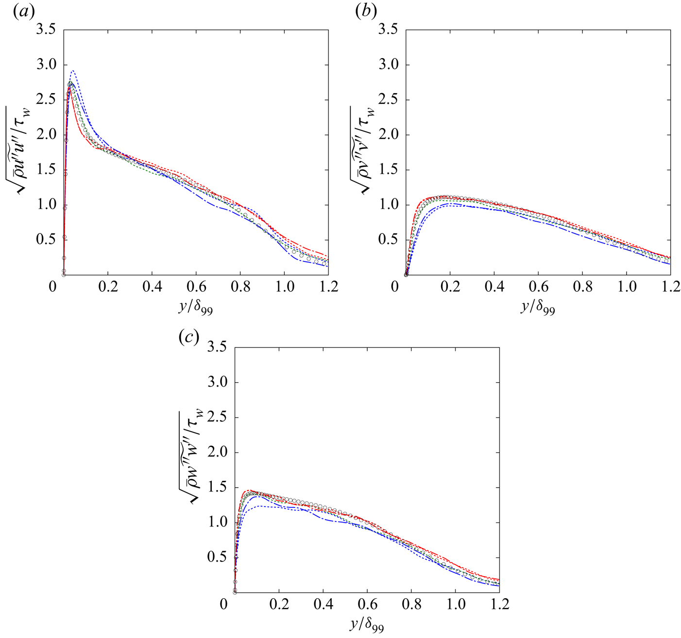
To examine whether the effect of the uphill diffusion extends to turbulence, figure 6 shows velocity fluctuation correlations. The notation $({\cdot })^{\prime \prime }$ indicates fluctuations about the Favre average and the fluctuations are non-dimensionalised by the wall shear stress. The DNS data of the incompressible constant-property turbulent boundary layer of Schlatter & Örlü (Reference Schlatter and Örlü2010) at $Re_{\tau } = 492$ is also included in the figure. The velocity fluctuation correlations of the present DNS are similar to those of the incompressible DNS data, indicating that at the relatively modest Mach number of the present study the qualitative characteristics of momentum diffusion are similar to those of the incompressible flow; however, for the cold-wall case the incompressible flow correlations slightly underpredict the present streamwise correlations and overpredict the wall-normal and spanwise correlations. In addition, the velocity fluctuation correlations of the four cases exhibiting uphill diffusions do not differ from the case in which uphill diffusion does not occur. This agreement among results in cases with and devoid of uphill diffusion indicates that the variation in the mass fraction due to the uphill diffusion does not significantly affect velocity turbulent fluctuation correlations.

Figure 6.

Velocity fluctuations in (a) streamwise, (b) wall-normal and (c) spanwise directions in uniform initial composition cases. The legend the same as in figure 4. Circles represent the DNS results from the incompressible constant-property boundary layer study of Schlatter & Örlü (Reference Schlatter and Örlü2010).

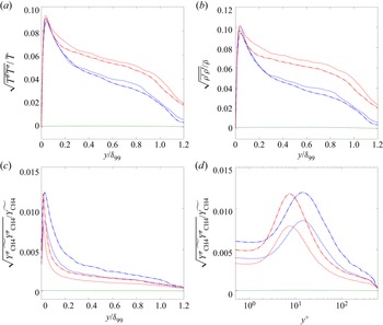
Figure 7 depicts fluctuation correlations of $T$, $\rho$ and $Y_{\text {CH}_{4}}$. The $T$ and $\rho$ fluctuation correlations are shown as a function of $y/\delta _{99}$ and the $Y_{\text {CH}_{4}}$ fluctuation correlation is shown as a function of either $y/\delta _{99}$ or $y^{+}$. These correlations are non-dimensionalised by the local values at each $y$ location. Without uphill diffusion these correlations are almost null because the profiles of $\tilde {T}/T_{w}$, $\bar {\rho }/\rho _{w}$ and $\widetilde {Y_{\text {CH}_{4}}}$ are uniform in the wall-normal direction. All the other cases have a sharp $T$ correlation peak of similar magnitude at $y/\delta _{99}\simeq 0.05$, and the $T$ correlation gradually decreases up to $y/\delta _{99}=0.2$. These qualitative characteristics are similar to the $u$ correlations in figure 6. Remarkably, although there is a decrease from the peak at $y/\delta _{99}=0.05$ in all uphill diffusion cases, the correlations in the hotter-wall cases remain considerably larger than in the colder-wall cases indicating that the situation is not symmetric as far as the imposed $T_{w}$ and $T_{\infty }$. This lack of symmetry is attributed to the different boundary conditions at the wall versus the far-field: Dirichlet versus non-reflective, respectively. The comparison between $T$ fluctuation correlation and $\rho$ fluctuation correlations shows that they are similar in all cases. Although a real-gas equation of state is used here, for the purpose of an approximate functional-dependence analysis, the perfect gas law is used showing that

(3.1)

\begin{equation} ( \bar{p}+p^{\prime}) \approx( \bar{\rho} +\rho^{\prime}) R( \tilde{T}+T^{\prime\prime}),\end{equation}

where $R=R_{u}( \sum _{\alpha =1}^{2}Y_{\alpha }/m_{\alpha })$ is the gas constant. Equation (3.1) is averaged in the homogeneous $(x,z)$ plane, resulting in

(3.2)

\begin{equation} \bar{p}\approx\bar{p}R\tilde{T}+\overline{\rho^{\prime} RT^{\prime\prime}}.\end{equation}

Substituting (3.2) into (3.1), one obtains

(3.3)

\begin{equation} p^{\prime}\approx\bar{\rho}RT^{\prime\prime}+\rho^{\prime}R\tilde{T}. \end{equation}

As $p^{\prime }$ is so small as to be negligible compared with $\bar {\rho }RT^{\prime \prime }$ and $\rho ^{\prime }R\tilde {T}$ (not shown), then

(3.4)

\begin{equation} 0\approx\bar{\rho}RT^{\prime\prime}+\rho^{\prime}R\tilde{T}, \end{equation}

so that

(3.5)

\begin{equation} \frac{\rho^{\prime}}{\bar{\rho}}\approx{-}\frac{T^{\prime\prime} }{\tilde{T}}, \end{equation}

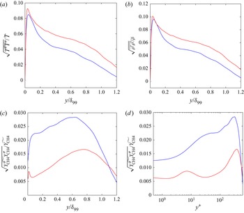
explaining the similarity between the $T$ and $\rho$ fluctuation correlations, and the fact that the $\rho$ correlations mainly depend on the $T$ correlations. The $Y_{\text {CH}_{4}}$ fluctuation correlation also has a peak around $y/\delta _{99}=0.05$ for all cases other than T-300-300-CH4-50-50, but after the correlations relax away from the wall those in the colder-wall cases remain larger than those in the hotter-wall cases; however, the difference between colder- and hotter-wall cases is not as large as for the temperature fluctuation correlations. Of note, the correlations do not relax to null values even for $y^{+}>20$ where the gradient of the mean mass fraction is almost null (see figure 5). This result indicates that uphill diffusion occurs even far from the wall. Essentially, if the fluid composition remains uniform past the imposed initial condition, the mass fraction should not fluctuate even in turbulent flows. Therefore, the $Y_{\text {CH}_{4}}$ fluctuations are also due to the uphill diffusion which renders the mass fraction nonuniform.

Figure 7.

Fluctuation correlations of (a) temperature, (b) density and (c,d) mass fraction of methane. Mass fraction profiles are shown as a function of the outer scaling $y/\delta _{99}$ (c) and as a function of the wall unit $y^{+}$ (d). The legend the same as in figure 4.

3.2.3. Species-mass diffusion balance in the mean flow field

The $\widetilde {Y_{\text {CH}_{4}}}$ profiles revealed that uphill diffusion occurs in the cases where there is a gradient in $\tilde {T}/T_{w}$. To elucidate the reason of the development of the species mass fraction gradient, the diffusion balance is investigated.

For the purpose of this analysis, the species-$\alpha$ conservation equation ((A4) shown in Appendix A) is averaged in the homogeneous ($x,z)$ plane and because through averaging the derivatives in the homogeneous directions are null, the following equation holds:

(3.6)

\begin{align} &\frac{\partial}{\partial t}(\bar{\rho}\widetilde{Y_{\alpha}}) +\frac{\partial}{\partial y}\left[ \bar{\rho} \widetilde{Y_{\alpha}}\tilde{v}+\bar{\rho} \widetilde{Y_{\alpha}^{\prime\prime}v^{\prime\prime}}- \overline{\rho Y_{\alpha}(D_{T,\alpha}) \frac{\partial T}{\partial y}}-\overline{\rho Y_{\alpha} (D_{p,\alpha}) \frac{\partial p}{\partial y}}\right.\nonumber\\ &\quad \left.-\sum_{\beta=1}^{N-1} \overline{\rho\left(D_{\alpha\beta}^{\prime} \frac{m_{\alpha}}{m_{\beta}}\right) \frac{\partial Y_{\beta}}{\partial y}}\right] =0. \end{align}

Equation (3.6) shows that the species-$\alpha$ mass flux for the mean flow field is given by

(3.7)

\begin{equation} J_{mean}(y)=\bar{\rho}\widetilde{Y_{\alpha}}\tilde{v}+\bar{\rho} \widetilde{Y_{\alpha}^{\prime\prime}v^{\prime\prime}}-\overline{\rho Y_{\alpha}( D_{T,\alpha}) \frac{\partial T}{\partial y} }-\overline{\rho Y_{\alpha}( D_{p,\alpha}) \frac{\partial p}{\partial y}}-\sum_{\beta=1}^{N-1}\overline{\rho\left( D_{\alpha\beta }^{\prime}\frac{m_{\alpha}}{m_{\beta}}\right) \frac{\partial Y_{\beta} }{\partial y}}, \end{equation}

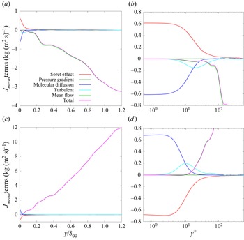
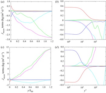
where the first term is the mean flow flux, the second term is the turbulent flux, the third term is the Soret flux, the fourth term is the pressure gradient flux (barodiffusion term) and the fifth term is the molecular diffusion flux.

Figure 8 shows the profiles of these five terms for CH$_{4}$ as a function of either $y/\delta _{99}$ or $y^{+}$ in T300-600-CH4-50-50 and T600-300-CH4-50-50. The mean flow flux in absolute value is large up to $y^{+}\simeq 100$ in both cases, a fact which is traced to the temperature difference between the wall and the far-field. For example, for T600-300-CH4-50-50, because the wall temperature is hotter than the fluid, the fluid receives heat from the wall, the heated fluid expands, the expansion causes an upward velocity in the wall-normal direction and the upward velocity causes the large mean flow flux. The opposite occurs in T300-600-CH4-50-50. However, the mean flow flux is small near the wall for $y^{+}\lesssim 10$, and the Soret flux and the molecular diffusion flux become there dominant. As the variation in $\widetilde {Y_{\text {CH}_{4}}}$ occurs only near the wall, this result indicates that the Soret effect and the molecular diffusion fluxes are related to this variation. Thus, the physics of the mass fraction gradient can be explained as follows. At the initial condition, $\widetilde {Y_{\text {CH}_{4}}}$ is uniform but $\tilde {T}$ has a gradient because the wall temperature is different from that in the far-field. The occurrence of $\boldsymbol {\nabla } T$ induces the Soret flux and its absolute value becomes large near the wall due to the large temperature gradient in the wall vicinity as shown in figure 4. The coefficient $D_{T,\alpha }$ is negative, and $\boldsymbol {\nabla } T$ is positive for T300-600-CH4-50-50 and negative for T600-300-CH4-50-50. Therefore, for T300-600-CH4-50-50 the Soret flux becomes positive and for T600-300-CH4-50-50 it becomes negative, as shown in figure 8. Thus, for T300-600-CH4-50-50 the Soret effect decreases the concentration of methane near the wall, whereas for T600-300-CH4-50-50 it enriches the fluid with methane near the wall. Once $\boldsymbol {\nabla } Y_{\text {CH}_{4}}$ occurs, it induces a molecular diffusion flux in the opposite direction. As the molecular diffusion flux is proportional to the $\boldsymbol {\nabla } Y_{\text {CH}_{4}}$, the molecular diffusion flux becomes significant to balance the Soret flux. Although not shown, the results of the species-mass flux for T300-600-CH4-25-25 and T600-300-CH4-25-25 are qualitatively the same as those for T300-600-CH4-50-50 and T600-300-CH4-50-50, respectively.

Figure 8.

Species-mass flux of the mean flow field as a function of the outer scaling $y/\delta _{99}$ (a,c) and as a function of the wall unit $y^{+}$ (b,d) for cases (a,b) T300-600-CH4-50-50 and (c,d) T600-300-CH4-50-50.

3.2.4. Flow structures

Investigation of turbulent statistics and species-mass diffusion balance revealed that uphill diffusion occurs due to the Soret effect. As a result, the mass fraction has a gradient and fluctuates even when the initial composition is uniform. To understand the flow physics of the species-mass diffusion in the flow field, fluctuation data of $u$, $T$ and $Y_{\text {CH}_{4}}$ are extracted in several planes. In addition, for the purpose of discussing the role of the Soret effect on species-mass diffusion, the divergence of the Soret flux

(3.8)

\begin{equation} \frac{\partial}{\partial x_{j}}\left( -\rho Y_{\alpha}( D_{T,\alpha })\frac{\boldsymbol{\nabla} T}{T}\right) =\boldsymbol{\nabla}\left( \frac{-\rho Y_{\alpha }(D_{T,\alpha})}{T}\right) \boldsymbol{{\cdot}} \boldsymbol{\nabla} T+\frac{-\rho Y_{\alpha}(D_{T,\alpha})}{T}{\cdot}{\nabla}^{2}T, \end{equation}

is considered. The first and second terms are proportional to $\boldsymbol {\nabla } T$ and $\nabla ^{2}T$, respectively. To determine which of the two terms imparts its features on the fluctuating flow structures, both $\boldsymbol {\nabla } T$ and $\nabla ^{2}T$ visualisations were examined. 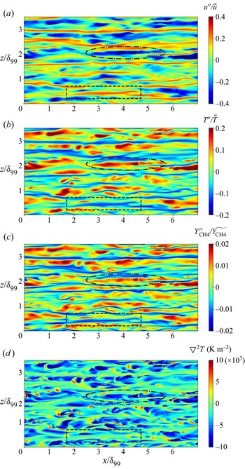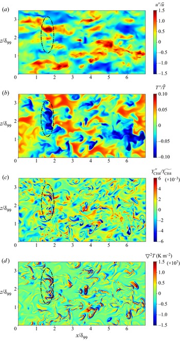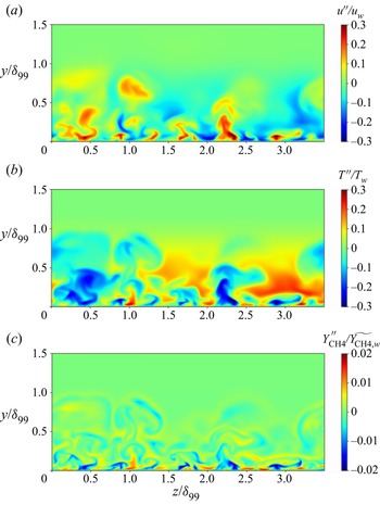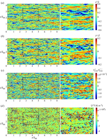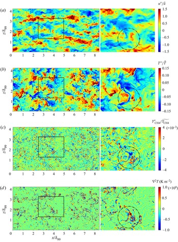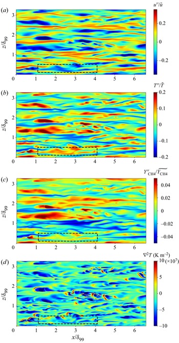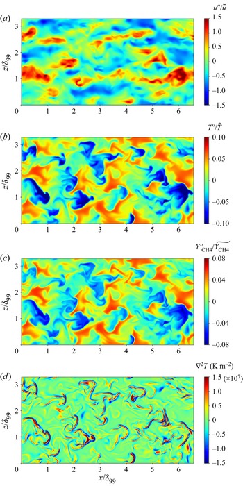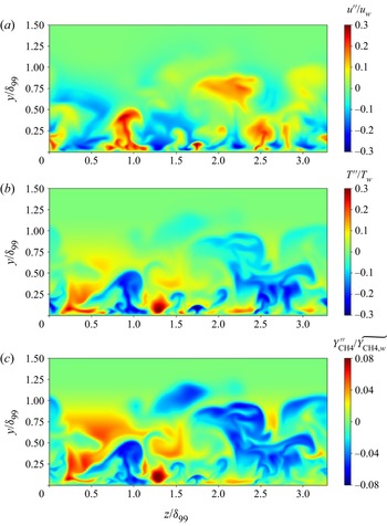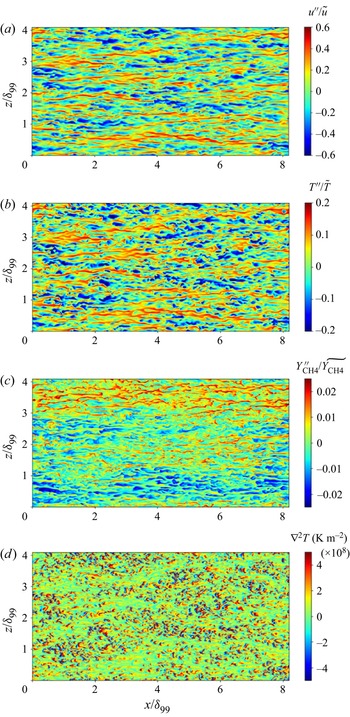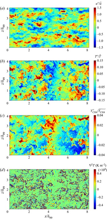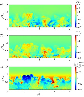No visual correlation was detected between $\boldsymbol {\nabla } T$ and the fluctuations, and thus only the $\nabla ^{2}T$ field is displayed. Instantaneous snapshot contours of T300-600-CH4-50-50 are shown in figures 9–11, and those of T600-300-CH4-50-50 are shown in figures 12–14. The region of the square box with a solid black line is enlarged and shown on the right in figures 12 and 13. 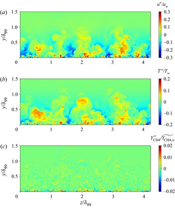Figure 9 shows contours in a wall-parallel plane at $y^{+}=10$, which is representative of the near-wall region; figure 10 shows data at $y^{+}=250$, which is located at the centre of the boundary layer; and figure 11 illustrates contours in a cross-flow plane at $x/\delta _{99}=2.87$. Likewise, figures 12 and 13 show contours at $y^{+}=10$ and $250$, respectively; figure 14 shows data at $x/\delta _{99}=3.47$. The fluctuations in the wall-parallel planes are non-dimensionalised by the local mean values at each $y^{+}$ location, and those in the cross-flow planes are non-dimensionalised by the wall values.

Figure 9.

Instantaneous snapshot at $Re_{\tau } \approx 500$ in the $y^{+}=10$ ($y/\delta _{99}=0.02$) wall-parallel plane for T300-600-CH4-50-50: (a) streamwise velocity, (b) temperature, (c) mass fraction of methane and (d) Laplacian of temperature.

Figure 10.

Instantaneous snapshot at $Re_{\tau } \approx 500$ in the $y^{+}=250$ ($y/\delta _{99}=0.5$) wall-parallel plane for T300-600-CH4-50-50: (a) streamwise velocity, (b) temperature, (c) mass fraction of methane and (d) Laplacian of temperature.

Figure 11.

Instantaneous snapshot at $Re_{\tau } \approx 500$ in the $x/\delta _{99}=2.87$ for T300-600-CH4-50-50: (a) streamwise velocity, (b) temperature and (c) mass fraction of methane.

Figure 12.

Instantaneous snapshot at $Re_{\tau } \approx 500$ in the $y^{+}=10$ ($y/\delta _{99}=0.02$) wall-parallel plane for T600-300-CH4-50-50: (a) streamwise velocity, (b) temperature, (c) mass fraction of methane and (d) Laplacian of temperature.

Figure 13.

Instantaneous snapshot at $Re_{\tau } \approx 500$ in the $y^{+}=250$ ($y/\delta _{99}=0.5$) wall-parallel plane for T600-300-CH4-50-50: (a) streamwise velocity, (b) temperature, (c) mass fraction of methane and (d) Laplacian of temperature.

Figure 14.

Instantaneous snapshot at $Re_{\tau } \approx 500$ in the $x/\delta _{99}=3.47$ plane for T600-300-CH4-50-50: (a) streamwise velocity, (b) temperature and (c) mass fraction of methane.

The $u$ field at $y^{+}=10,$ illustrated in figure 9 for T300-600-CH4-50-50 exhibits the typical streaky structures. Because the wall is moving and the far-field is at rest, the high-speed streaks are accompanied by the upward ($v^{\prime \prime }>0$) vertical transport of the near-wall fluid, and can be interpreted as ejection events. The low-speed streaks are accompanied by the downward ($v^{\prime \prime }<0$) vertical transport of the upper fluid, and can be interpreted as sweep events. Similar streaky structures were observed in many DNS of compressible boundary layers (Duan et al. Reference Duan, Beekman and Martín2010, Reference Duan, Beekman and Martín2011; Pirozzoli & Bernardini Reference Pirozzoli and Bernardini2011; Kawai Reference Kawai2019). The results show that $T$ and $Y_{\text {CH}_{4}}$ have the almost same flow field as $u$. The comparison among $u$, $T$ and $Y_{\text {CH}_{4}}$ reveals that the high temperature and high concentration of CH$_{4}$ streaks appear in the same region as the low-speed streaks and vice versa. The coincidence of the streaky structures indicates that all fluctuations of $u$, $T$ and $Y_{\text {CH}_{4}}$ are induced by the same mechanism. It is well known that $u$ and $T$ fluctuations are caused by the ejection and sweep events (Wallace, Eckelmann & Brodkey Reference Wallace, Eckelmann and Brodkey1972; Nagano & Tagawa Reference Nagano and Tagawa1988; Park et al. Reference Park, Wallace, Wu and Moin2012; Wallace Reference Wallace2016). In T300-600-CH4-50-50, the high-speed and low-temperature fluids are ejected, and the low-speed and high-temperature fluids are swept. Thus, the $Y_{\text {CH}_{4}}$ field indicates that fluids of small CH$_{4}$ concentration are ejected and large CH$_{4}$ concentration are swept. The explanation of the ejection and sweep regarding $Y_{\text {CH}_{4}}$ is consistent with the mean profile. Although the initial composition is uniform in this case, the Soret effect decreases $Y_{\text {CH}_{4}}$ near the wall as shown in figure 5. Therefore, the $Y_{\text {CH}_{4}}$ fluctuations are correlated to dynamics fluctuations such as the ejection and sweep events near the wall. The fluctuation of $Y_{\text {CH}_{4}}$ is also correlated to ${\nabla }^{2}T$, but its correlation is weaker than those discussed already. The comparison between $Y_{\text {CH}_{4}}$ and ${\nabla }^{2}T$ shows that the high concentration accompanied by the sweep is correlated to the negative ${\nabla }^{2}T$ region. For example, in the region surrounded by the black dash-dotted line, a red-coloured streaky structure is observed in the $Y_{\text {CH}_{4}}$ field, and a blue-coloured structure is observed in the ${\nabla }^{2}T$ field. In contrast, in the region included in the black dashed line square box, a blue-colored streaky structure is observed in the $Y_{\text {CH}_{4}}$ field, but ${\nabla }^{2}T$ in that region is almost null. This result reveals that the $Y_{\text {CH}_{4}}$ field is less correlated to ${\nabla }^{2}T$ than to dynamics fluctuations indicating that the $Y_{\text {CH}_{4}}$ fluctuation mainly depends on dynamics fluctuations rather than the Soret effect near the wall.

The similarity between the $u$, $T$ and $Y_{\text {CH}_{4}}$ fields does not hold at the centre of the boundary layer, as shown in figure 10. The $u$ field at $y^{+}=250$ has streaky structures and their spanwise spacing and streamwise length are wider and shorter than those at $y^{+}=10$. The $T$ field also has streaky structures, but they are less clear and some long structures in the spanwise direction appear, such as a low-temperature structure surrounded by the black dash-dotted line. The dissimilarity between the $u$ and $T$ at the centre of the boundary layer were also reported in past studies (Pirozzoli & Bernardini Reference Pirozzoli and Bernardini2011; Toki & Bellan Reference Toki and Bellan2021). In the $Y_{\text {CH}_{4}}$ field, streaky structures no longer exist and its fluctuations are finer than those of $u$ and $T$. For example, the comparison in the region surrounded by the black dash-dotted line reveals that the $Y_{\text {CH}_{4}}$ is finely fluctuating in the large low-temperature structure. This difference in a structure of the fluctuations indicates that the cause of the fluctuation in the mass fraction is induced by a different mechanism from those in $u$ and $T$. However, the $Y_{\text {CH}_{4}}$ field is similar to the ${\nabla }^{2}T$ field at $y^{+}=250$. In particular, the $Y_{\text {CH}_{4}}$ field has almost the same structure as the ${\nabla }^{2}T$ in the region where the ${\nabla }^{2}T$ is large in absolute value. As mentioned previously, one of the terms issued from the Soret flux in $\boldsymbol {J}_{\alpha }$ is proportional to ${\nabla }^{2}T$, and thus this similar structure indicates that the $Y_{\text {CH}_{4}}$ fluctuations largely depend on the Soret effect at the centre of the boundary layer.

The observation of the wall-parallel planes indicated that the $Y_{\text {CH}_{4}}$ fluctuations are caused by dynamics fluctuations near the wall, whereas they are mainly induced by the Soret flux at the centre of the boundary layer. The difference in the flow physics between the wall vicinity and the centre can also be observed in the cross-flow plane. Figure 11 shows that $u$ and $T$ in the cross-flow plane exhibit strongly fluctuations in the entire boundary layer. In addition, some fluctuations near the wall extend and connect to those in the central region of the boundary layer. The extension of the fluctuations indicates that the fluctuations in the central region are attributable to the ejection and sweep events near the wall. In contrast, $Y_{\text {CH}_{4}}$ is strongly fluctuating only near the wall, and its fluctuations become weaker after $y/\delta _{99}\simeq 0.2$. Furthermore, the fluctuations near the wall do not extend towards the far-field. This result indicates that the fluctuations at the centre are not correlated to the ejection and sweep events. This absence of the correlation can be explained by the mean profile of the mass fraction. As shown in figure 5, $\boldsymbol {\nabla } \widetilde {Y_{\text {CH}_{4}}}$ is very small after $y/\delta _{99}\simeq 0.2$. Therefore, the upward and downward motions do not involve the mixing of different concentration fluids.

The qualitative characteristic of the flow field in T600-300-CH4-50-50 is the same as T300-600-CH4-50-50. The wall-parallel planes at $y^{+}=10$ in figure 12 show that independent of the wall versus free-stream temperature in these cases, $u$, $T$ and $Y_{\text {CH}_{4}}$ have streaky structures and their flow fields are similar to each other. However, the correlations between the ${\nabla }^{2}T$ and the other flow fields are weaker here. For example, in the region included in the black dashed line square box, a blue-coloured structure is observed in the $Y_{\text {CH}_{4}}$ field, and a red-coloured structure is observed in the ${\nabla }^{2}T$ field. In contrast, in the region surrounded by the black dash-dotted line, a red-coloured structure is observed in the $Y_{\text {CH}_{4}}$ field, but ${\nabla }^{2}T$ is almost null. This result indicates that the $Y_{\text {CH}_{4}}$ fluctuations primarily depend on dynamics fluctuations near the wall, akin to T300-600-CH4-50-50. The similarity between the $u$, $T$ and $Y_{\text {CH}_{4}}$ at $y^{+}=250$ is also weaker for T600-300-CH4-50-50, as illustrated in figure 13. In addition, the $Y_{\text {CH}_{4}}$ field has finer structures than those of $u$ and $T$ such as in the region surrounded by the black dash-dotted line. The structures in the $Y_{\text {CH}_{4}}$ field are similar to the ${\nabla }^{2}T$ field, this being an indication that the $Y_{\text {CH}_{4}}$ fluctuations largely depend on the Soret effect, similar to T300-600-CH4-50-50. The cross-flow plane fields in figure 14 show that $Y_{\text {CH}_{4}}$ strongly fluctuates only near the wall, and its flow physics can be explained in the same way as for T300-600-CH4-50-50.

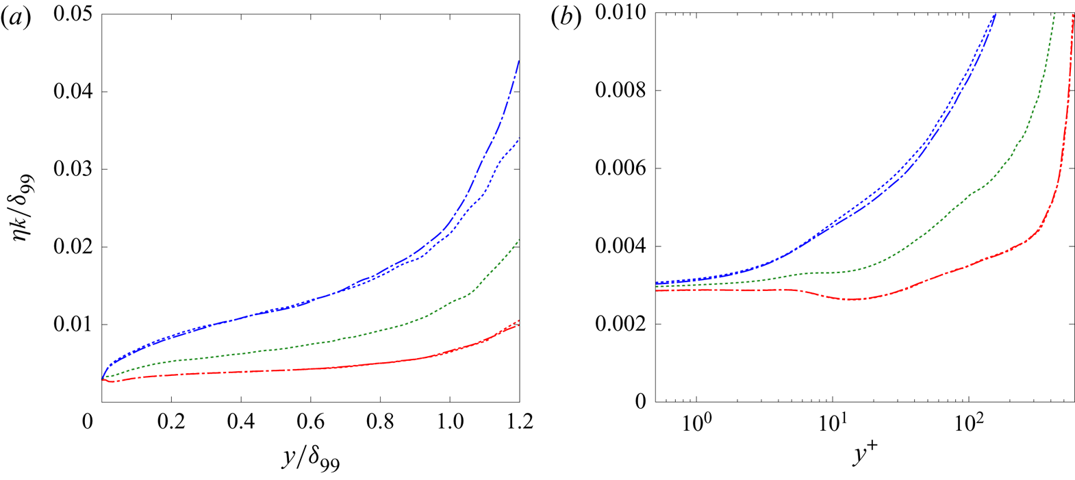
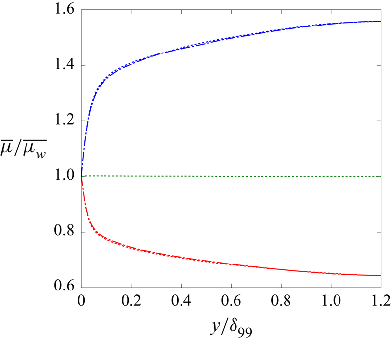
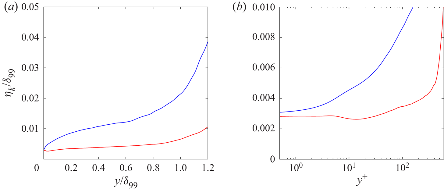
The comparison of the flow fields between T300-600-CH4-50-50 (figures 9–11) and T600-300-CH4-50-50 (figures 12–14) indicates that in all planes the hotter-wall case has finer fluctuations that the colder-wall case. To discuss the difference in the size of flow structures, figure 15 compares the Kolmogorov scales (non-dimensionalised by $\delta _{99}$) among the uniform initial composition cases. The Kolmogorov scale monotonically and substantially increases from the wall in the colder-wall cases, whereas it only slightly varies in the hotter-wall case. As the result, at $y^{+}=10$ the Kolmogorov scale in the colder-wall case is twice as large as in the hotter-wall case. Moreover, at $y/\delta _{99}=0.5$ ($y^{+}=250$) the ratio of the Kolmogorov scale between the hotter- and colder-wall cases becomes greater than 3. This result indicates that the finer structures in the hotter-wall case should be attributed to the smaller Kolmogorov scale. 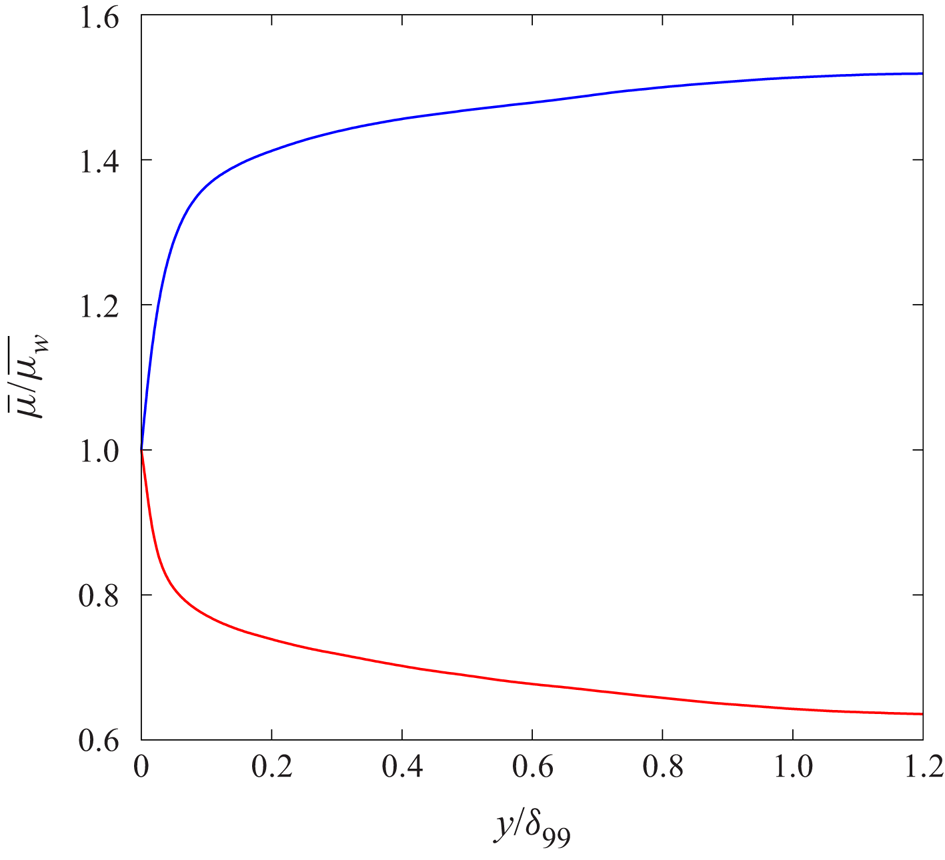According to (2.7), the Kolmogorov scale depends on $\bar {\rho },$ depicted scaled by $\overline {\rho }_{w}$ in figure 4, and $\bar {\mu },$ portrayed scaled by $\overline {{\mu }_{w}}$ in figure 16. Figures 4 and 16 show that $\bar {\rho }$ monotonically decreases and $\bar {\mu }$ increases from the wall in the colder case. Both of these variations enlarge the Kolmogorov scale. In contrast, $\bar {\rho }$ monotonically increases and $\bar {\mu }$ decreases from the wall in the hotter-wall case, and these variations reduce the Kolmogorov scale. As both of $\rho$ and $\mu$ strongly depend on $T$, the difference in the $\bar {\rho }$ and $\bar {\mu }$ profiles is due to the opposite temperature conditions. Thus, the asymmetry in temperature conditions between the colder- and hotter-wall cases induces the difference in the size of flow structures.

Figure 15.

Kolmogorov scale profiles in cases with uniform initial composition as a function of (a) the outer scaling $y/\delta _{99}$ and (b) the wall unit $y^{+}$. The legend is the same as in figure 4.

Figure 16.

Profile of the mean viscosity in cases with uniform initial composition. The legend is the same as in figure 4.

The above analysis shows that when there is a temperature gradient between wall and free stream a binary-species fluid of initially uniform composition is not equivalent to a single-species fluid. That is, even if the initial composition is uniform, resembling a single species, a non-uniform composition quickly develops. In addition, the two situations of colder and hotter wall compared with the free stream are not symmetric as far as the temperature or species mass fraction fluctuations. The specific non-symmetric characteristics make the scales of all variables smaller in the hotter-wall case. Computationally, this explains why a considerably finer grid in the wall-normal direction was necessary for the hotter-wall cases compared with the colder-wall cases, as listed in table 1. As the Kolmogorov scale substantially increases in the direction normal to the wall in the colder-wall case, the required grid resolution becomes coarser in that direction; therefore, a stretched grid can be applied in the wall-normal direction. In contrast, the Kolmogorov scale varies only slightly in the hotter-wall case, and thus a much finer grid in the wall-normal direction is required to obtain DNS resolution. In principle, for the colder-wall case the grid resolution requirements in the streamwise and spanwise directions can also accommodate a coarser grid away from the wall, however the present simulations are performed on a structured grid in those directions and the resolution has been selected to suit the more stringent requirements of the hotter-wall cases.

The conclusion is that should there be a temperature gradient between wall and free stream, even when the composition is initially uniform it rapidly becomes non-uniform. This observation motivates the study of initially non-uniform compositions, addressed next.

3.3. Effects of wall versus fluid temperature for non-uniform binary-species initial composition

According to § 3.2, a non-uniform initial composition in the wall-normal direction is the prevalent case in boundary layer flows; analyses of cases T300-600-CH4-25-50 and T600-300-CH4-25-50 allow the elucidation of the physics in the more typical cases of unequal composition. All analyses are conducted at $Re_{\tau }\approx 500$, as listed in table 1.

3.3.1. Mean profiles

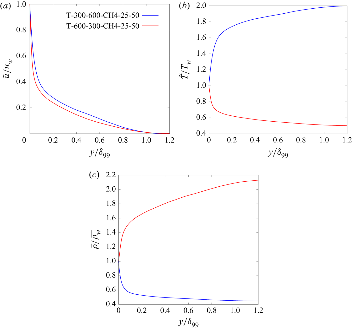
Figure 17 shows mean profiles of $\tilde {u}/u_{w}$, $\tilde {T}/T_{w}$ and $\bar {\rho }/\rho _{w}$ for the two cases with the non-uniform initial composition. The qualitative characteristics of these profiles are similar to the cases with uniform initial composition: $\tilde {u}/u_{w}$ monotonically decreases from the wall to the far-field, $\tilde {T}/T_{w}$ monotonically increases and decreases from the wall in the colder- and hotter-wall cases, respectively, and $\bar {\rho }/\rho _{w}$ monotonically decreases or increases reflecting the $\tilde {T}/T_{w}$ profile. These same qualitative characteristics indicates that the mean profiles are insensitive to the variation in the the mass fraction in the wall-normal direction.

Figure 17.

Mean profiles of (a) streamwise velocity, (b) temperature and (c) density in cases with non-uniform initial composition.

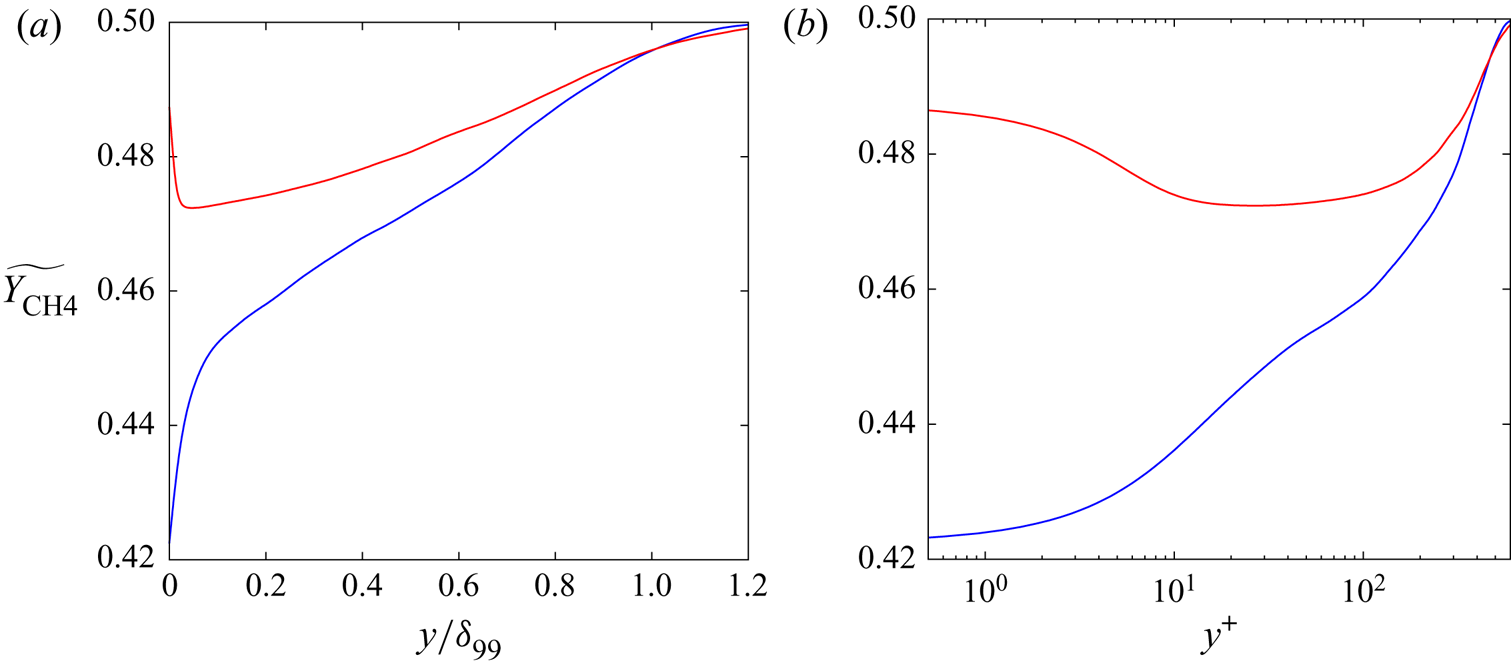
To investigate species-mass diffusion, figure 18 depicts mean profiles of $\widetilde {Y_{\text {CH}_{4}}}$. In the colder-wall case, T-300-600-CH4-25-50, $\widetilde {Y_{\text {CH}_{4}}}$ monotonically increases from the wall to the far-field. As the initial $\widetilde {Y_{\text {CH}_{4}}}$ value at the wall is smaller than that at the far-field, this monotonic increase is easily expectable. However, the hotter-wall case $\widetilde {Y_{\text {CH}_{4}}}$ profile is considerably different from the colder situation as it decreases from the wall to $y^{+}\simeq 10$, and further increases to the far-field. As a monotonic variation in the $\widetilde {Y_{\text {CH}_{4}}}$ is imposed at the initial condition, the minimum value reached at $y^{+}=10$ and the plateau at this minimum value for $10\lesssim y^{+}\lesssim 50$ is a counterintuitive result because both colder- and hotter-wall cases have similar mass fraction profiles at the initial condition. In fact, comparison between the two cases shows that $\widetilde {Y_{\text {CH}_{4}}}$ in the colder-wall case is smaller than in the hotter-wall case in the entire of the boundary layer. This result indicates that methane is less diffused in the colder-wall case. To understand the different physics in these two situations, turbulent fluctuations are examined in § 3.3.2 and the species diffusion balance in the mean flow is assessed in § 3.3.3.

Figure 18.

Mean profiles of mass fraction of methane in non-uniform initial composition cases as a function of (a) the outer scaling $y/\delta _{99}$ and as a function of (b) the wall unit $y^{+}$. The legend the same as figure 17.

3.3.2. Turbulent fluctuation correlations

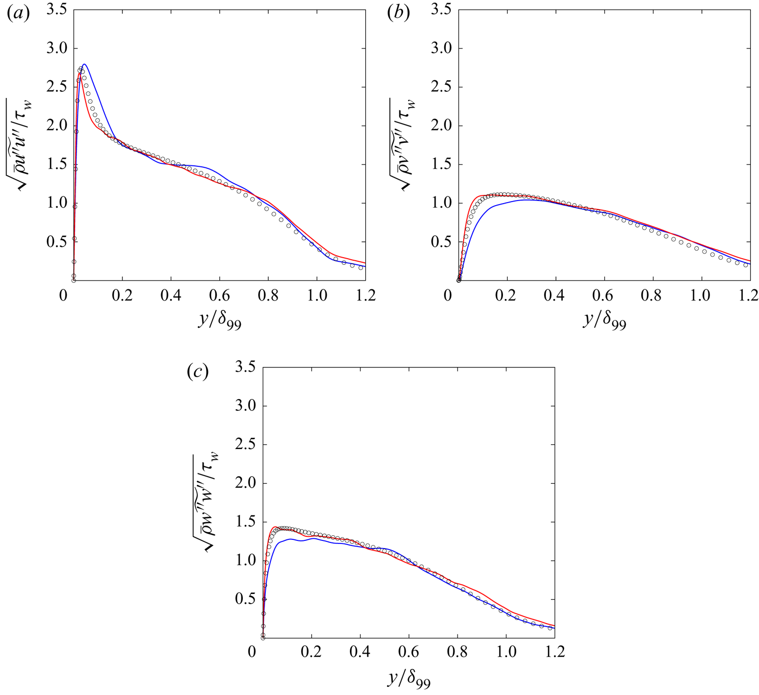
To examine the effect of non-uniform composition on turbulence, figure 19 compares velocity fluctuation correlations with those of the incompressible constant-property boundary layer of Schlatter & Örlü (Reference Schlatter and Örlü2010) at $Re_{\tau }=492$. The comparison reveals that the velocity fluctuations agree well with the incompressible data, however, in the cold-wall case, near the wall the incompressible results slightly underpredict the streamwise correlations whereas they overpredict the wall-normal and spanwise correlations. This result is similar to that of the uniform initial composition discussed in § 3.2.2.

Figure 19.

Velocity fluctuations in (a) streamwise, (b) wall-normal and (c) spanwise directions in non-uniform initial composition cases. The legend the same as in figure 17. Circles represent the DNS results from the incompressible constant-property boundary layer study of Schlatter & Örlü (Reference Schlatter and Örlü2010).

Figure 20 shows fluctuation correlations of $T$, $\rho$ and $Y_{\text {CH}_{4}}$. The $T$ correlation profile has a sharp peak, slightly larger for the hot-wall case compared with the colder-wall case, at $y/\delta _{99}=0.044$ for the colder-wall case and at $y/\delta _{99}=0.033$ for the hotter-wall case, and sharply decreases to $y/\delta _{99}\simeq 0.2$ in the colder-wall case whereas it gradually decreases to $y/\delta _{99}\simeq 0.2$ in the hotter-wall case. The $\rho$ correlation is quite similar to the $T$ correlation, except that the difference in peaks between colder- and hotter-wall cases is smaller. These qualitative characteristics of $T$ and $\rho$ correlations are similar to, but not the same as those of the uniform composition cases, indicating that the variation in the mass fraction has a small influence on the $T$ and $\rho$ correlations. However, the $Y_{\text {CH}_{4}}$ fluctuation correlations are substantially different from the uniform composition cases. The $Y_{\text {CH}_{4}}$ correlation has a peak at $y/\delta _{99}\simeq 0.6$ in the colder-wall case, and $y/\delta _{99}=0.8$ in the hotter-wall case. These peak locations are different from the uniform composition cases, which have peaks at $y/\delta _{99}=0.05$ this being the location of the $T$ and $\rho$ correlations. Moreover, in the uniform composition cases the shape of the profiles was similar in the colder- versus the hotter-wall cases, whereas here it is dissimilar. Thus, these results imply that the mechanism producing the $Y_{\text {CH}_{4}}$ fluctuation correlation is different in the non-uniform and the uniform composition cases.

Figure 20.

3.3.3. Species-mass diffusion balance in the mean flow

Consideration of $\widetilde {Y_{\text {CH}_{4}}}$ revealed that in the hotter-wall case it decreases from the wall value at locations $y^{+}\lesssim 10$. To elucidate the reason of the counterintuitive profile near the wall, the diffusion balance is investigated.

Figure 21 shows the profiles of the five terms in (3.7) for $\widetilde {Y_{\text {CH}_{4}}}$ as a function of either $y/\delta _{99}$ or $y^{+}$ in T300-600-CH4-25-50 and T600-300-CH4-25-50. Similarly to the uniform composition cases, the mean flow flux in absolute value is large for $y^{+}\gtrsim 100$ in both cases. In the $y^{+}\gtrsim 100$ region, the turbulent flux is relatively large and the other terms are negligible. The turbulent flux in the hotter-wall case (T600-300-CH4-25-50) has a sign switch from positive to negative at $y^{+}\simeq 20$ resulting from the sign switch of $\boldsymbol {\nabla }\widetilde {Y_{\text {CH}_{4}}}$ at this location. For $y^{+}\lesssim 10$, the Soret flux and the molecular diffusion flux become dominant, similar to the uniform composition cases. Therefore, the unique $\widetilde {Y_{\text {CH}_{4}}}$ profile near the wall in the hotter-wall case should be explained by these latter two terms.

Figure 21.

Species-mass flux of the mean flow field as a function of the outer scaling $y/\delta _{99}$ (a,c) and as a function of the wall unit $y^{+}$ (b,d) for cases (a,b) T300-600-CH4-25-50 and (c,d) T600-300-CH4-25-50. The legend is the same as in figure 8.

In the present non-uniform cases, at the initial condition $\widetilde {Y_{\text {CH}_{4}}}$ monotonically increases from the wall to the far-field. Therefore, as the simulation is initiated the CH$_{4}$ mass diffusion flux is directed toward the wall. As mentioned in § 3.2.3, the Soret flux is also directed towards the wall in the hotter-wall case due to the signs of $\boldsymbol {\nabla } T$ and $D_{T,\alpha },$ which is negative. As the magnitude of the Soret flux strongly depends on $\boldsymbol {\nabla } T$ which is largest near the wall, the Soret flux becomes larger near the wall. Molecular mass diffusion and Soret fluxes are both directed towards the wall, and the magnitude of their sum, which given the negligible barodiffusion contribution represents the total flux, is largest in the vicinity of the wall. The larger total flux enriches CH$_{4}$ near the wall against $\boldsymbol {\nabla }\widetilde {Y_{\text {CH}_{4}}}$. As the molecular mass diffusion flux depends on $\boldsymbol {\nabla }\widetilde {Y_{\text {CH}_{4}}}$, its direction is switched near the wall to balance the Soret flux. This physics provides the reason for the counterintuitive near-wall $\widetilde {Y_{\text {CH}_{4}}}$ variation in the hotter-wall case. The plateau region identified in figure 18 over $10\lesssim y^{+}\lesssim 100$ corresponds to the region in which the molecular mass diffusion and Soret flux balance in such a way as to yield a constant $\widetilde {Y_{\text {CH}_{4}}}$ and at larger $y^{+}$, $\widetilde {Y_{\text {CH}_{4}}}$ increases to the value specified at the free stream; further discussions are provided in § 3.3.4. In the colder-wall case, the direction of the Soret flux is opposite to that of mass diffusion, and thus the Soret flux prevents a high concentration of CH$_{4}$ region forming near the wall. As a result, in the colder-wall case $\widetilde {Y_{\text {CH}_{4}}}$ remains smaller than the hotter-wall case, as shown in figure 18.

3.3.4. Flow structures

Similarly to the uniform composition cases, to understand the result of the species-mass diffusion on the flow field initiated with non-uniform composition, fluctuation data of $u$, $T$, $Y_{\text {CH}_{4}}$ and $\nabla ^{2}T$ are extracted in several planes. Instantaneous snapshot contours of T300-600-CH4-25-50 are shown in figures 22–24, and the equivalent for T600-300-CH4-25-50 are shown in figures 25–27. Figures 22 and 23 show contours in a wall-parallel plane at $y^{+}=10$ and $250$, respectively, whereas figure 24 illustrates contours in a cross-flow plane at $x/\delta _{99}=2.69$. Likewise, figures 25 and 26 show contours at $y^{+}=10$ and $250$; figure 14 shows data at $x/\delta _{99}=3.35$.

Figure 22.

Instantaneous snapshot at $Re_{\tau } \approx 500$ in the $y^{+}=10$ ($y/\delta _{99}=0.02$) wall-parallel plane for T300-600-CH4-25-50: (a) streamwise velocity, (b) temperature, (c) mass fraction of methane and (d) Laplacian of temperature.

Figure 23.

Instantaneous snapshot at $Re_{\tau } \approx 500$ in the $y^{+}=250$ ($y/\delta _{99}=0.5$) wall-parallel plane for T300-600-CH4-25-50: (a) streamwise velocity, (b) temperature, (c) mass fraction of methane and (d) Laplacian of temperature.

Figure 24.

Instantaneous snapshot at $Re_{\tau } \approx 500$ in the $x/\delta _{99}=2.69$ for T300-600-CH4-25-50: (a) streamwise velocity, (b) temperature and (c) mass fraction of methane.

Figure 25.

Instantaneous snapshot at $Re_{\tau } \approx 500$ in the $y^{+}=10$ ($y/\delta _{99}=0.02$) wall-parallel plane for T600-300-CH4-25-50: (a) streamwise velocity, (b) temperature, (c) mass fraction of methane and (d) Laplacian of temperature.

Figure 26.

Instantaneous snapshot at $Re_{\tau } \approx 500$ in the $y^{+}=250$ ($y/\delta _{99}=0.5$) wall-parallel plane for T600-300-CH4-25-50: (a) streamwise velocity, (b) temperature, (c) mass fraction of methane and (d) Laplacian of temperature.

Figure 27.

Instantaneous snapshot at $Re_{\tau } \approx 500$ in the $x/\delta _{99}=3.35$ plane for T600-300-CH4-25-50: (a) streamwise velocity, (b) temperature and (c) mass fraction of methane.

In the colder-wall case (T300-600-CH4-25-50), the $u$, $T$ and $\nabla ^{2}T$ fields at $y^{+}=10$ are similar to the uniform composition cases with the colder wall (T300-600-CH4-50-50 and T300-600-CH4-25-25). Both of $u$ and $T$ have streaky structures as evident in figure 22, and their flow fields are similar to each other. The comparison between $T$ and $\nabla ^{2}T$ shows that the negative $\nabla ^{2}T$ region is correlated to the high-temperature region, but $\nabla ^{2}T$ is almost null in the low-temperature region. These qualitative characteristics of $u$, $T$ and $\nabla ^{2}T$ are the same as the uniform composition cases. However, the $Y_{\text {CH}_{4}}$ field is dissimilar from the $u$ and $T$ fields, although it also exhibits streaky structures. For example, in the region included in the black dashed-line square box, a high-temperature and low-velocity streak is observed. In contrast, there is no streaky structure of $Y_{\text {CH}_{4}}$ in the same region. The same dissimilarity of the $Y_{\text {CH}_{4}}$ was also reported in the previous DNS (Toki & Bellan Reference Toki and Bellan2021), and it is because the species-mass flux deviates from Fick's law due to the Soret effect.

For T300-600-CH4-25-50, figure 23 shows that structures of the $u$, $T$ and $\nabla ^{2}T$ fields at $y^{+}=250$ are also similar to the uniform composition case shown in figure 10, and only the $Y_{\text {CH}_{4}}$ field is different. The comparison between the four fields reveals that the $Y_{\text {CH}_{4}}$ field is quite similar to that of $T$, and it is largely different from the $\nabla ^{2}T$ field and $\boldsymbol {\nabla } T$. This result indicates that the $Y_{\text {CH}_{4}}$ field is independent of the Soret effect, and the mechanism of the $Y_{\text {CH}_{4}}$ fluctuations is similar to that of the $T$ fluctuations. It is well known that the $T$ fluctuations are induced by the dynamics fluctuations and, thus, the $Y_{\text {CH}_{4}}$ fluctuations are also induced by the dynamics fluctuations in the non-uniform composition case. This consideration is supported by observation of the cross-flow plane. The contours in the cross-flow planes (figure 24) show that the $Y_{\text {CH}_{4}}$ fluctuations approximately at the centre of the boundary layer are connected to those near the wall like the $u$ and $T$ fluctuations. This connection indicates that the $Y_{\text {CH}_{4}}$ fluctuations are correlated to the ejection and sweep events.

In the hotter-wall case (T600-300-CH4-25-50), the qualitative characteristics of the $u$, $T$ and $\nabla ^{2}T$ fields are the same as the uniform composition cases with the hotter wall. However, there are some differences in the $Y_{\text {CH}_{4}}$ field. Figure 25 shows that at $y^{+}=10$, $Y_{\text {CH}_{4}}$ has streaky structures and their shape is similar to the $u$ and $T$ fields. Therefore, this field indicates that the $Y_{\text {CH}_{4}}$ fluctuations near the wall are also induced by the dynamics fluctuations. However, the comparison among $u$, $T$ and $Y_{\text {CH}_{4}}$ shows that the $Y_{\text {CH}_{4}}$ field is less similar to the other fields than in the uniform composition cases. In contrast, the $Y_{\text {CH}_{4}}$ field, shown in figure 26 at $y^{+}=250$, is quite similar to the $T$ field. The low $Y_{\text {CH}_{4}}$ region is correlated to the high $T$ region and vice versa. The reduced similarity at $y^{+}=10$ can be explained by the mean $Y_{\text {CH}_{4}}$ profile in a cross-flow plane. The mean $Y_{\text {CH}_{4}}$ profile depicted in figure 18 already revealed that the $\widetilde {Y_{\text {CH}_{4}}}$ is nearly constant between $y^{+}=10$ and $50$ because its minimum value results from the Soret effect which acts in concert with molecular mass diffusion. In this region, the upper fluid and the lower fluid have almost the same CH$_{4}$ concentration, and thus there is no corresponding $Y_{\text {CH}_{4}}$ fluctuation to those of the dynamics fluctuations. This consideration is supported by the cross-flow plane visualisations (figure 27). The $Y_{\text {CH}_{4}}$ contour in the cross-flow plane reveals that the $Y_{\text {CH}_{4}}$ is strongly fluctuating for $y/\delta _{99}\gtrsim 0.5$, whereas the fluctuations are extremely weak for $y/\delta _{99}\lesssim 0.3$. This explains why at $y^{+}=10$ the $Y_{\text {CH}_{4}}$ fluctuations are less similar to those of $u$ and $T: \widetilde {Y_{\text {CH}_{4}}}$ becomes almost constant in the $10\lesssim y^{+}\lesssim 50$ region due to the Soret effect resulting in very reduced $Y_{\text {CH}_{4}}$ fluctuations.

Of note, similarly to the uniform composition cases, the scales are much smaller for the hotter-wall compared with the colder-wall cases. Figures 28 and 29 presenting the Kolmogorov scale and the $\bar {\mu }$ profiles, respectively, reveal that these quantities have qualitative characteristics that are almost the same for the non-uniform and uniform composition cases. Therefore, the much smaller scales in the hotter-wall case with the non-uniform composition can be also explained by the smaller Kolmogorov scale due to the different temperature conditions.

Figure 28.

Kolmogorov scale profiles in cases with non-uniform initial composition as a function of the outer scaling $y/\delta _{99}$ (a) and as a function of the wall unit $y^{+}$ (b). The legend is the same as in figure 17.

Figure 29.

Mean viscosity profiles in cases with non-uniform initial composition. The legend is the same as in figure 17.

4. Conclusions

DNS of temporal binary-species boundary layers at high-pressure has been conducted to investigate the influence of the Soret effect on the flow physics. Thus, the simulations encompassed both colder and hotter walls compared with the free stream and three different kinds of initial mixtures: uniform and of equal compositions, uniform but of unequal compositions and non-uniform compositions as function of the wall-normal coordinate. The initially uniform composition conditions have been studied to determine the approximations that would be made should such a situation be represented by a single-species fluid. The working fluid was a mixture of nitrogen and methane and the free-stream pressure was 60 atm. After showing that a self-similarity becomes established in the streamwise velocity, temperature and mass fraction, all simulations have been analysed at a similar value of the friction Reynolds number, $Re_{\tau }\approx 500$. Examination of these boundary layers elucidated the influence of the Soret effect under different conditions and showed that this effect induced uphill diffusion, a phenomenon never before associated with thermophoresis. Whereas uphill diffusion has been shown in the past to only occur when there at least three chemical species present, the present study shows that in the presence of thermophoresis it can also occur when there are only two chemical species.

For the initially uniform composition, irrespective of whether it was an equal or an unequal distribution between the two species, the mean profile of the mass fraction acquired a gradient in the wall-normal direction. As regular diffusion would not induce a mass fraction gradient in these cases, this result indicates that uphill diffusion occurs in the flow field. The velocity fluctuation correlations are similar to those of the incompressible constant-property boundary layers, and thus they are insensitive to uphill diffusion. Investigation of the mass fraction fluctuation correlations revealed that a maximum value appears near the wall but the correlations are not null over the entire boundary layer height, indicating that uphill diffusion occurs even far from the wall. These qualitative characteristics regarding mean profiles and turbulent statistics are the same whether for equal and unequal compositions, indicating that flow physics in initially uniform boundary layers is similar irrespective of the composition. The species-mass diffusion balance for mean flow fields showed that the Soret flux and the molecular diffusion flux become dominant near the wall. The Soret flux enriches the fluid with methane near the wall in the hotter-wall cases, whereas it decreases the concentration of methane near the wall in colder-wall cases. As molecular diffusion flux is proportional to the mass fraction gradient, the former, which is initially null over the entire boundary layer height, also becomes significant to balance the Soret flux. The flow structures in the wall-parallel plane are similar for the velocity, temperature and mass fraction fields near the wall. This result indicates that the mass fraction fluctuations near the wall are induced by dynamics fluctuations such as the ejection and sweep in the same way that the velocity and the temperature fluctuate. In contrast, the mass fraction field is not similar to either the velocity or temperature at the centre of the boundary layer, indicating that the mass fraction fluctuations are induced by a different mechanism from those of velocity and temperature. As the Laplacian of the temperature field shows similar behaviour to the mass fraction fluctuation field, this similarity indicates that the latter are induced by the Soret effect. Although the magnitude of the temperature difference between wall and far field is the same in the colder- and hotter-wall situations, the direction of the temperature flux near the wall crucially affects the scale of the fluctuations and the hotter-wall cases exhibit much smaller scales than the colder-wall cases.

The difference between colder- and hotter-wall situations becomes even larger for an initially non-uniform composition; because initially uniform compositions quickly become non-uniform, the means that this non-uniformity accelerates the differences between colder- and hotter-wall situations. The mean mass fraction of methane monotonically increases from the wall to the far-field in the colder-wall case, whereas the hotter-wall case does not have its minimum value at the wall despite the initial profile which specifies a minimum at the wall. Instead, the mean mass fraction of methane in the hotter-wall case decreases from the wall in its immediate vicinity, then reaches a minimum at which a plateau develops and thereafter increases to the far-field. Although both of the colder- and hotter-wall cases have similar mass fraction profiles at the initial condition, the mass fraction of methane in the colder-wall case is smaller than the hotter-wall case in the entire of the boundary layer. This result indicates that methane diffuses less in the colder-wall case. The fluctuation correlations profiles showed that a maximum peak appears around the centre of the boundary layer unlike the situation for the uniform composition cases. Similar to the uniform composition cases, the species-mass diffusion balance revealed that the Soret flux and the molecular diffusion flux are dominant near the wall. As due to the large temperature gradient the Soret flux is strong near the wall, in the hotter-wall case this flux provokes a molecular mass diffusion flux which enriches methane near the wall against the mass fraction gradient. As a result, the mean mass fraction of methane in the hotter-wall case does not achieve a minimum value at the wall. In contrast, the direction of the Soret effect is opposite in the colder-wall case, and thus the Soret effect prevents high concentration of methane from reaching the near-wall region. Visualisations of the flow-field fluctuations showed that in parallel planes to the wall the mass fraction field is not similar to the velocity and temperature fields near the wall, but the similarity between mass fraction and temperature is recovered at the centre of the boundary layer in both of the colder- and hotter-wall cases. These observations of the colder-wall case agree with those of a previous study (Toki & Bellan Reference Toki and Bellan2021). However, visualisations in a cross-flow plane indicate differences between the colder-wall and hotter-wall cases in that the mass fraction fluctuates in the entire of the boundary layer in the colder-wall case whereas in the hotter-wall case the fluctuations near the wall are much weaker than at the boundary layer centre. These weaker fluctuations are due to the mass fraction mean profile plateau near the wall. Analogous to the initial composition situation, fluctuation scales are much smaller in the hotter-wall than in the colder-wall situation, a fact traced to the smaller Kolmogorov scale.

The results from this study show that when a wall is at a different temperature from the adjacent multi-species fluid, the multi-species fluid cannot be approximated in the wall boundary layer by a single-species fluid. The temperature difference between wall and far-field governs the evolution of the fluid composition which becomes different from its initial composition. Starting with the same initial composition and same magnitude of the temperature difference between wall and free stream, hotter and colder walls induce different compositions in the boundary layer due to the opposite sign of the temperature gradient. Moreover, the flow structure for the hotter wall exhibits much smaller structures than in the colder-wall equivalent case. This indicates that the temperature gradient could potentially be used to control the composition of the adjacent fluid, in particular to avoid unwanted species, such as those producing corrosion or initiating carbon producing reactions, from reaching the wall, as well as control the flow structure in that region. Of note, at the large Reynolds number values of the practical applications compared with those reachable here in DNS, the dynamic characteristic time will decrease whereas the diffusional time remains the same, leading to even larger temperature gradients, as shown by Sciacovelli & Bellan (Reference Sciacovelli and Bellan2019). This fact combined with the larger temperature gradients already existing in practical systems implies that thermophoretic effects will be considerably more significant than those showed in the present study.

Acknowledgements

Computational resources were provided by the JPL Supercomputing Center, by NASA Advanced Supercomputing at Ames Research Center under the T3 program directed by Dr M. M. Rogers.

Funding

This work was conducted at the California Institute of Technology (Caltech) and sponsored by the Department of Energy (DOE), Basic Energy Sciences (BES) under the direction of Dr W. Sisk, with the DOE grant number DE-SC0002679.

Declaration of interests

The authors report no conflict of interest.

Appendix A. Governing equations

The governing equations are the conservation equations complemented by the equation of state (EOS).

A.1. Differential conservation equations

The conservation equations for multi-species flow (Okong'o & Bellan Reference Okong'o and Bellan2002) are

(A1)

\begin{gather} \frac{\partial\rho}{\partial t}+\frac{\partial}{\partial x_{j}}[\rho u_{j}] =0, \end{gather}

(A2)

\begin{gather}\frac{\partial}{\partial t}(\rho u_{i})+ \frac{\partial }{\partial x_{j}}[\rho u_{i}u_{j}+p\delta_{ij}-\sigma_{ij}] =0, \end{gather}

(A3)

\begin{gather}\frac{\partial}{\partial t}(\rho e_{t}) +\frac{\partial }{\partial x_{j}}[ (\rho e_{t}+p) u_{j}-u_{i}\sigma _{ij}+q_{j}] =0, \end{gather}

(A4)

\begin{gather}\frac{\partial}{\partial t}(\rho Y_{\alpha}) +\frac{\partial }{\partial x_{j}}[\rho Y_{\alpha}\ u_{j}+J_{\alpha j}] =0, \end{gather}

where $\alpha \in \lbrack 1,N-1]$, $t$ denotes the time, $x$ is a Cartesian coordinate, $u$ is the velocity, $e_{t}=e+u_{i}u_{i}/2$ is the total energy (i.e. internal energy, $e$, plus kinetic energy), $Y_{\alpha }$ is the mass fraction of species $\alpha$, $N$ is the number of species, $\boldsymbol {q}$ is the heat flux and $\boldsymbol {J}_{\alpha }$ is $\alpha$-species mass flux. The subscripts $i$ and $j$ refer to spatial coordinates. The Newtonian viscous stress tensor $\sigma _{ij}$ is written as follows:

(A5a,b)

\begin{equation} \sigma_{ij}=\mu\left( 2S_{ij}-\dfrac{2}{3}S_{kk}\delta_{ij}\right) ,\quad S_{ij}=\dfrac{1}{2}\left( \dfrac{\partial u_{i}}{\partial x_{j}} +\dfrac{\partial u_{j}}{\partial x_{i}}\right) , \end{equation}

where $\mu$ is the viscosity and $S_{ij}$ is the strain-rate tensor.

Owing to the different constitutive relations used for expressing $\boldsymbol {J}_{\alpha }$ and $\boldsymbol {q}$, (A1)–(A4) under high-$p$ conditions have ultimately a different form from that used under atmospheric-$p$ conditions. The present $\boldsymbol {J}_{\alpha }$ and $\boldsymbol {q}$ expressions are based on the full matrices of mass-diffusion coefficients and thermal-diffusion factors derived by Harstad & Bellan (Reference Harstad and Bellan2004a). As (A1) is solved, only a set of independent $(N-1)$ species equations rather than the set of $N$ dependent species is considered; in these $(N-1)$ equations, the original molar-fraction fluxes and the heat flux were rewritten to account for only $(N-1)$ gradients. The final form is

(A6)

\begin{gather} \boldsymbol{J}_{\alpha}={-}\rho\left[ Y_{\alpha}( D_{T,\alpha}) \frac{\boldsymbol{\nabla} T}{T}+Y_{\alpha}( D_{p,\alpha}) \frac{\boldsymbol{\nabla} p} {p}+\sum_{\beta=1}^{N-1}\left( D_{\alpha\beta}^{\prime}\frac{m_{\alpha} }{m_{\beta}}\right) \boldsymbol{\nabla} Y_{\beta}\right] , \end{gather}

(A7)

\begin{gather}\boldsymbol{q}={-}\lambda\boldsymbol{\nabla} T+\sum_{\alpha=1}^{N-1}\boldsymbol{J}_{\alpha}\left[ \left( \frac{h_{\alpha}}{m_{\alpha}}-\frac{h_{N}}{m_{N}}\right) -R_{u}T\left( \frac{\bar{\alpha}_{T,\alpha}^{b}}{m_{\alpha}}-\frac {\bar{\alpha}_{T,N}^{b}}{m_{N}}\right) \right] , \end{gather}

where

(A8a,b)

\begin{gather} D_{T,\alpha}={-}\sum_{\beta=1}^{N}\bar{\alpha}_{T,\beta}^{b}\mathbb{D} _{\beta\alpha},\quad D_{p,\alpha}=\frac{p}{R_{u}T}\sum _{\beta=1}^{N}v_{\beta}\mathbb{D}_{\beta\alpha}, \end{gather}

(A9)

\begin{gather} D_{\alpha\gamma}=\sum_{\beta=1}^{N}\mathbb{D}_{\alpha\beta}\alpha _{D\beta\gamma}, \end{gather}

(A10)

\begin{gather}\bar{\alpha}_{T,\alpha}^{b}=\sum_{\beta=1}^{N}X_{\beta}\alpha_{T,\beta \alpha}^{b}, \end{gather}

(A11)

\begin{gather}D_{\alpha\beta}^{\prime}=D_{\alpha\beta}-\left( 1-\frac{m_{\beta}}{m_{N} }\right) \left(\sum_{\gamma=1}^{N-1}D_{\alpha\gamma}X_{\gamma}\right). \end{gather}

Here, $T$ is the temperature; $X_{\alpha }=Y_{\alpha }m/m_{\alpha }$ is the molar fraction; $m_{\alpha }$ is the species molar mass; $m$ is the mixture molar mass, $m=\sum _{\gamma =1}^{N}m_{\gamma }X_{\gamma }; v_{\alpha }=(\partial v/\partial X_{\alpha })_{T,p,X_{\beta }(\beta \neq \alpha )}$ is the partial molar volume, where the molar volume is $v=1/n$ and $n=\rho /m$ is the molar density; $h_{\alpha }=(\partial h/\partial X_{\alpha })_{T,p,X_{\beta }(\beta \neq \alpha )}$ is the partial molar enthalpy, where the molar enthalpy is $h=G-T(\partial G/\partial T)_{p,X}$ with $G$ being the Gibbs energy$; R_{u}$ is the universal gas constant; $D_{\alpha \gamma }$ are the pairwise mass diffusion coefficients; $\alpha _{T,\alpha \beta }^{b}$ are the binary thermal diffusion factors; and $\lambda$ is the thermal conductivity. The mass-diffusion factors, $\alpha _{D\alpha \beta },$ are calculated from thermodynamics as

(A12)

\begin{equation} \alpha_{D\alpha\beta}\equiv\dfrac{1}{R_{u}T}X_{\alpha}\dfrac{\partial \mu_{\alpha}}{\partial X_{\beta}}=(\delta_{\alpha\beta}-\delta_{\alpha N})+X_{\alpha}(R_{\alpha\beta}-R_{\alpha N}), \end{equation}

with $1\leqslant \alpha \leqslant N$, $1\leqslant \beta \leqslant N-1$, and

(A13)

\begin{equation} R_{\alpha\beta}\equiv\frac{\partial\ln\gamma_{\alpha}}{\partial X_{\beta}}, \end{equation}

with $1\leqslant \alpha \leqslant N$, $1\leqslant \beta \leqslant N$. In (A12) and (A13), $\mu _{\alpha }$ is the chemical potential of species $\alpha$ written in terms of $N-1$ species; $\gamma _{\alpha }\equiv \varphi _{\alpha }/\varphi _{\alpha }^{o}$ where $\varphi$ is the fugacity coefficient written in terms of $N$ species and the superscript $o$ denotes the pure ($X_{\alpha }=1)$ limit. More details are provided in Appendix A.3.

A.2. Equation of state

Equations (A1)–(A4) are coupled with a modified Peng–Robinson (PR) EOS introduced by Harstad et al. (Reference Harstad, Miller and Bellan1997)

(A14)

\begin{equation} p=\dfrac{R_{u}T\left(\displaystyle \sum_{\alpha=1}^{\alpha=N}X_{\alpha}\right) }{(v_{PR}-b_{mix})} -\dfrac{a_{mix}}{(v_{PR}^{2}+2b_{mix} v_{PR}-b_{mix}^{2})}.\end{equation}

Here, $v_{PR}$ is the molar PR volume, and $v=v_{PR}+v_{s}$ where $v_{s}$ is the volume shift introduced for improving the accuracy of the PR EOS at high pressure, and the $v_{s}$ computation was described in detail elsewhere (Okong'o, Harstad & Bellan Reference Okong'o, Harstad and Bellan2002).

Miscellaneous relationships relevant to the EOS are

(A15a,b)

\begin{equation} a_{mix}=\sum_{\alpha}\sum_{\gamma}X_{\alpha}X_{\gamma}a_{\alpha\gamma}(T), \quad b_{mix}=\sum_{\alpha}X_{\alpha}b_{\alpha}, \end{equation}

where indices do not follow the Einstein notation, and

(A16)

\begin{equation} a_{\alpha\gamma}=(1-k_{\alpha\gamma}^{\prime})\sqrt{\alpha_{\alpha\alpha }\alpha_{\gamma\gamma}}, \end{equation}

(A17)

\begin{align} \alpha_{\alpha\alpha}(T) & \equiv0.457236(R_{u}T_{c,\alpha})^{2}\nonumber\\ & \quad \times\frac{[ 1+c_{\alpha}(1-\sqrt{T_{red,\alpha}})]^{2} }{p_{c,\alpha}}, \end{align}

(A18)

\begin{equation} c_{\alpha}=0.37464+1.54226\varOmega_{\alpha}-0.26992\varOmega_{\alpha}^{2}, \end{equation}

where $T_{red,\alpha }\equiv T/T_{c,\alpha }, T_{c,\alpha }$ is the critical temperature and $\varOmega _{\alpha }$ is the acentric factor. In addition,

(A19)

\begin{gather} b_{\alpha}=0.077796\dfrac{R_{u}T_{c,\alpha}}{p_{c,\alpha}}, \end{gather}

(A20)

\begin{gather}T_{c,\alpha\gamma}=(1-k_{\alpha\gamma}) \sqrt{T_{c,\alpha}T_{c,\gamma}}\quad \text{with }k_{\alpha\alpha}=0, \end{gather}

(A21)

\begin{gather}v_{c,\alpha\gamma}=\dfrac{1}{8}( v_{c,\alpha}^{1/3}+v_{c,\gamma} ^{1/3})^{3}, \end{gather}

(A22)

\begin{gather}Z_{c,\alpha\gamma}=\dfrac{1}{2}( Z_{c,\alpha}+Z_{c,\gamma}), \end{gather}

(A23)

\begin{gather}p_{c,\alpha\gamma}=\dfrac{R_{u}T_{c,\alpha\gamma}Z_{c,\alpha \gamma}}{v_{c,\alpha\gamma n}}, \end{gather}

with $T_{red,\alpha \gamma }\equiv T/T_{c,\alpha \gamma },Z_{c,\alpha }$ being the critical compression factor with the compression factor defined as $Z=p/(\rho TR_{u}/m)$, $v_{c,\alpha }$ being the critical volume and $p_{c,\alpha }$ being the critical pressure. Here $k_{\alpha \gamma }$ is an empirical mixing parameter. The relationship between parameters $k_{\alpha \gamma }$ and $k_{\alpha \gamma }^{\prime }$ is

(A24)

\begin{equation} (1-k_{\alpha\gamma})=(1-k_{\alpha\gamma}^{\prime})\frac{(v_{c,\alpha }v_{c,\gamma})^{1/2}}{v_{c,\alpha\gamma}}. \end{equation}

For N$_{2}$/CH$_{4}$, $k^{\prime } = 0.0311$ (Knapp et al. Reference Knapp, Döring, Oellrich, Plöcker and Prausnitz1982).

A.3. Transport properties

Matrix elements $\mathbb {D}_{\beta \gamma }$ of (A8a,b)–(A9) are the solution of the mixing rules (Harstad & Bellan Reference Harstad and Bellan2004a)

(A25)

\begin{equation} \sum_{\beta=1}^{N}\left[ \delta_{\alpha\beta}- (1-\delta_{\alpha\beta}) X_{\beta}\frac{\bar{\mathcal{D}}_{\alpha}}{\mathcal{D}_{\alpha\beta }^{b}}\right] \frac{\mathbb{D}_{\beta\gamma}}{X_{\beta}}= \bar{\mathcal{D}}_{\alpha}\frac{(\delta_{\alpha\gamma} -Y_{\alpha})}{X_{\alpha}}, \end{equation}

where

(A26)

\begin{equation} \bar{\mathcal{D}}_{\alpha}=1 \left/ \sum_{\substack{\beta=1 \\ \beta\neq\alpha}}^{N}\left(\dfrac{X_{\beta}}{\mathcal{D}_{\alpha \beta}^{b}}\right)\right. . \end{equation}

Solutions for $\mathbb {D}_{\beta \gamma }$ may be obtained by an approximate inversion (Ern & Giovangigli Reference Ern and Giovangigli1998) as follows:

(A27)

\begin{gather} \mathbb{D}_{\beta\gamma} \simeq X_{\beta}\mathbb{D}_{\beta\gamma}^{(1)}, \end{gather}

(A28)

\begin{gather}\mathbb{D}_{\alpha\beta}^{(1)} =\frac{( 1+Y_{\alpha }) }{X_{\alpha}}\mathcal{D}_{\alpha}^{{\ast}}\delta_{\alpha\beta}+( 1-\delta_{\alpha\beta}) \frac{\mathcal{D}_{\alpha}^{{\ast}} \mathcal{D}_{\beta}^{{\ast}}}{\mathcal{D}_{\alpha\beta}^{b}}-( \sigma_{\alpha}\mathcal{D}_{\alpha}^{{\ast}}+\sigma_{\beta}\mathcal{D}_{\beta }^{{\ast}}) +\sum_{\gamma=1}^{N}( Y_{\gamma}\sigma_{\gamma }\mathcal{D}_{\gamma}^{{\ast}}) , \end{gather}

(A29)

\begin{gather}\mathcal{D}_{\alpha}^{{\ast}} =( 1-Y_{\alpha}) \bar{\mathcal{D}}_{\alpha}, \end{gather}

(A30)

\begin{gather}\sigma_{\alpha} =\frac{m_{\alpha}}{m}(1+Y_{\alpha}) +\sum_{\substack{\beta=1\\ \beta\neq\alpha}}^{N}Y_{\beta} \frac{\mathcal{D}_{\beta}^{{\ast}}}{\mathcal{D}_{\alpha\beta}^{b}}, \end{gather}

where ${\mathcal {D}_{\alpha \beta }^{b}}$ is the full approximation binary-diffusion matrix. This method leads to a singularity when the mixture is composed of only one species (as, for instance, in pure fuel zones). In that case (A26) is no longer used and the diffusion coefficients are evaluated using the binary-diffusion matrix, by setting $\mathcal {D}_{\alpha }^{\ast }= \mathcal {D}_{\alpha N}^{b}$ where $N$ represents the index associated with the solvent. This method was tested against an exact Gauss inversion (not shown) and it gave the same results, with an additional gain in computational time. Defining $\mathcal {D} _{\alpha \beta }$ as the first approximation of the binary diffusion matrix and realising that the deviation of the ratio $\mathcal {D}_{\alpha \beta }^{b}/\mathcal {D}_{\alpha \beta }$ from unity is comparable to uncertainties in binary diffusion coefficients values (Harstad & Bellan Reference Harstad and Bellan2004a), we assume $\mathcal {D}_{\alpha \beta }^{b}=\mathcal {D}_{\alpha \beta }$. The computation of ${\mathcal {D}_{\alpha \beta }^{{}}}$ and $\alpha _{T,\alpha \beta }^{b}$ is described in the references of Masi et al. (Reference Masi, Bellan, Harstad and Okong'o2013) and Sciacovelli & Bellan (Reference Sciacovelli and Bellan2019) along with the other transport properties.

Appendix B. Numerical method

The differential equations combined with the EOS described in § A are numerically solved using a fourth-order explicit Runge–Kutta time integration and a sixth-order compact scheme spatial discretisation (Lele Reference Lele1992); the CFL number is 0.8. The conservation equations are first solved, and $T$ and $p$ are obtained as an iterative solution which satisfies both values of $\rho$ and $e$, as obtained from the conservation equations. In order to ensure time stability, the conservative variables were filtered using the eighth-order compact filter described elsewhere (Gaitonde & Visbal Reference Gaitonde and Visbal1998). Because the order of the filter is larger than that of the discretisation, no physical information is removed by the filter which only serves to remove unphysical fluctuations associated with long computer run times. In the past (Sciacovelli & Bellan Reference Sciacovelli and Bellan2019), a parametric study using several filter coefficients (0.45, 0.475 and 0.49) was conducted indicating that the value 0.49 was sufficiently large to ensure that the filter only acts on the shortest wavelengths that can be resolved on the grid and it does not affect the physical content of the data. The code was parallelised using three-dimensional domain decomposition and message passing. The tridiagonal solvers for the compact derivative scheme and the compact filter were efficiently parallelised using a well-established method (Muller & Scheerer Reference Muller and Scheerer1991). A flow chart of the code appears in figure 30.

Figure 30.

Flow chart of the code used in the simulations, where $t_{n}$ is the computational time at the $n$th step.

Appendix C. Streamwise and spanwise spectra

The grid resolutions of the present simulations satisfy the requirements of the Kolmogorov scale and the Batchelor scale, but these requirement can be insufficient as mentioned in § 2. Therefore, the one-dimensional spectra are assessed to check the grid resolutions. Figures 31 and 32 illustrate the streamwise and spanwise spectra, $E(k)$, of the three velocity components, the temperature and the mass fraction of methane, all computed near the wall ($y^{+}=10$) and the centre of the boundary layers ($y/\delta _{99}=0.5$). The spectra of all quantities show the smoothness associated with turbulent characteristics except for the small peak at the perturbation frequency and display excellent grid resolution because there is no energy accumulation at the smallest scales.

Figure 31.

One-dimensional spectra at $y^{+}=10$ for several cases: streamwise spectra of (a) $u$, (b) $v$, (c) $w$, (d) $T$, (e) $Y_{\text {CH}_{4}}$; spanwise spectra of (f) $u$, (g) $v$, (h) $w$, (i) $T$, (j) $Y_{\text {CH}_{4}}$. The legend is the same as in figure 2.

Figure 32.

One-dimensional spectra at $y/\delta _{99}=0.5$ for several cases: streamwise spectra of (a) $u$, (b) $v$, (c) $w$, (d) $T$, (e) $Y_{\text {CH}_{4}}$; spanwise spectra of (f) $u$, (g) $v$, (h) $w$, (i) $T$, (j) $Y_{\text {CH}_{4}}$. The legend is the same as in figure 2.

References

REFERENCES

Bae, J.H., Yoo, J.Y. & Choi, H. 2005 Direct numerical simulation of turbulent supercritical flows with heat transfer. Phys. Fluids 17, 105104.CrossRef Google Scholar

Bae, J.H., Yoo, J.Y. & McEligot, D.M. 2008 Direct numerical simulation of heated

$\mathrm {CO_{2}}$ flows at supercritical pressure in a vertical annulus at

$Re=8900$. Phys. Fluids 20, 055108.CrossRef Google Scholar

Ben Dakhlia, R., Giovangigli, V. & Rosner, D.E. 2002 Soret effects in laminar counterflow spray diffusion flames. Combust. Theor. Model. 6, 1–17.CrossRef Google Scholar

Castiglioni, G. & Bellan, J. 2018 On models for predicting thermodynamic regimes in high-pressure turbulent mixing and combustion of multi-species mixtures. J. Fluid Mech. 843, 536–574.CrossRef Google Scholar

Clusius, K. & Dickel, G. 1938 New process for separation of gas mixture and isotopes. Naturewiss 26, 546.CrossRef Google Scholar

Duan, L., Beekman, I. & Martín, M.P. 2010 Direct numerical simulation of hypersonic turbulent boundary layers. Part 2. Effect of wall temperature. J. Fluid Mech. 655, 419–445.CrossRef Google Scholar

Duan, L., Beekman, I. & Martín, M.P. 2011 Direct numerical simulation of hypersonic turbulent boundary layers. Part 3. Effect of Mach number. J. Fluid Mech. 672, 245–267.CrossRef Google Scholar

Duncan, J.B. & Toor, H.L. 1962 An experimental study of three component gas diffusion. AIChE J. 8 (1), 38–41.CrossRef Google Scholar

Ern, A. & Giovangigli, V. 1998 Thermal diffusion effects in hydrogen–air and methane–air flames. Combust. Theor. Model. 2, 349–372.CrossRef Google Scholar

Faith, L.E., Ackerman, G.H. & Henderson, H.T. 1971 Heat sink capability of jet a fuel: heat transfer and coking studies. S-14115, NASA CR-72951. Shell Development Co.Google Scholar

Gaitonde, D.V. & Visbal, M.R. 1998 High-order schemes for Navier–Stokes equations: algorithm and implementation into FDL3DI. In Air Force Research Lab Wright-Patterson AFB OH Air Vehicles Directorate AFRL-VA-WP-TR-1998-3060.CrossRef Google Scholar

Garcia-Ybarra, P.L. & Castillo, J.L. 1997 Mass transfer dominated by thermal diffusion in laminar boundary layers. J. Fluid Mech. 336, 379–409.CrossRef Google Scholar

Grcar, J.F., Bell, J. & Day, M. 2009 The Soret effect in naturally propagating, premixed, lean, hydrogen–air flames. Proc. Combust. Inst. 32, 1173–1180.CrossRef Google Scholar

Guo, J., Yang, X.I.A. & Ihme, M. 2022 Structure of the thermal boundary layer in turbulent channel flows at transcritical conditions. J. Fluid Mech. 934, A45.CrossRef Google Scholar

Harstad, K. & Bellan, J. 2004 a Mixing rules for multicomponent mixture mass diffusion coefficients and thermal diffusion factors. J. Chem. Phys. 120, 5664–5673.CrossRef Google Scholar PubMed

Harstad, K. & Bellan, J. 2004 b High-pressure binary mass-diffusion coefficients for combustion applications. Ind. Engng Chem. Res. 43, 645–654.Google Scholar

Harstad, K., Miller, R.S. & Bellan, J. 1997 Efficient high-pressure state equations. AIChE J. 43, 1605–1610.CrossRef Google Scholar

Jones, R.C. & Furry, W.H. 1946 The separation of isotopes by thermal diffusion. Rev. Mod. Phys. 18, 151–224.Google Scholar

Kawai, S. 2019 Heated transcritical and unheated non-transcritical turbulent boundary layers at supercritical pressures. J. Fluid Mech. 865, 563–601.CrossRef Google Scholar

Kim, K., Hickey, J. & Scalo, C. 2019 Pseudophase change effects in turbulent channel flow under transcritical temperature conditions. J. Fluid Mech. 871, 52–91.Google Scholar

Knapp, H., Döring, R., Oellrich, L., Plöcker, U. & Prausnitz, J.M. 1982 Vapor-Liquid Equilibria for Mixtures of Low Boiling Substances, vol. VI. Dechema.Google Scholar

Kozul, M., Chung, D. & Monty, J.P. 2016 Direct numerical simulation of the incompressible temporally developing turbulent boundary layer. J. Fluid Mech. 796, 437–472.Google Scholar

Lee, J., Jung, S.Y., Sung, H.J. & Zaki, T.A. 2013 Effect of wall heating on turbulent boundary layers with temperature-dependent viscosity. J. Fluid Mech. 726, 196–225.CrossRef Google Scholar

Lele, S.K. 1992 Compact finite difference schemes with spectral-like resolution. J. Comput. Phys. 103 (1), 16–42.CrossRef Google Scholar

Liu, V.C. 1959 On the separation of gas mixtures by suction of thermal diffusion boundary layer. Q. J. Mech. Appl. Maths 12, 1–13.Google Scholar

Ma, P.C., Yang, X.I.A. & Ihme, M. 2018 Structure of wall-bounded flows at transcritical conditions. Phys. Rev. Fluids 3, 034609.CrossRef Google Scholar

Martín, M.P. 2004 DNS of hypersonic turbulent boundary layers, 34th AIAA Fluid Dynamics Conference and Exhibit. AIAA Paper 2004-2337.CrossRef Google Scholar

Masi, E., Bellan, J., Harstad, K.G. & Okong'o, N.A. 2013 Multi-species turbulent mixing under supercritical-pressure conditions: modelling, direct numerical simulation and analysis revealing species spinodal decomposition. J. Fluid Mech. 721, 578–626.CrossRef Google Scholar

Moin, P. & Mahesh, K. 1998 Direct numerical simulation: a tool in turbulence research. Annu. Rev. Fluid Mech. 30, 539–578.CrossRef Google Scholar

Muller, S.M. & Scheerer, D. 1991 A method to parallelize tridiagonal solvers. Parallel Comput. 17, 181–188.CrossRef Google Scholar

Nagano, Y. & Tagawa, M. 1988 Statistical characteristics of wall turbulence with a passive scalar. J. Fluid Mech. 196, 157–185.CrossRef Google Scholar

Nemati, H., Patel, A., Boersma, B.J. & Pecnik, R. 2015 Mean statistics of a heated turbulent pipe flow at supercritical pressure. Intl J. Heat Mass Transfer 83, 741–752.CrossRef Google Scholar

Nemati, H., Patel, A., Boersma, B.J. & Pecnik, R. 2016 The effect of thermal boundary conditions on forced convection heat transfer to fluids at supercritical pressure. J. Fluid Mech. 800, 531–556.CrossRef Google Scholar

Okong'o, N. & Bellan, J. 2002 Consistent boundary conditions for multicomponent real gas mixtures based on characteristics wave. J. Comput. Phys. 176, 330–344.CrossRef Google Scholar

Okong'o, N., Harstad, K. & Bellan, J. 2002 Direct numerical simulation of

$\mathrm {O_{2} /H_{2}}$ temporal mixing layers under supercritical conditions. AIAA J. 40, 914–926.CrossRef Google Scholar

Park, G.I., Wallace, J.M., Wu, X. & Moin, P. 2012 Boundary layer turbulence in transitional and developed states. Phys. Fluids 24, 035105.CrossRef Google Scholar

Patel, A., Boersma, B.J. & Pecnik, R. 2016 The influence of near-wall density and viscosity gradients on turbulence in channel flows. J. Fluid Mech. 809, 793–820.CrossRef Google Scholar

Patel, A., Boersma, B.J. & Pecnik, R. 2017 Scalar statistics in variable property turbulent channel flows. Phys. Rev. Fluids 2, 084604.CrossRef Google Scholar

Peeters, J.W.R., Pecnik, R., Rohde, M., Hagen, T.H.J.J.V.D. & Boersma, B.J. 2016 Turbulence attenuation in simultaneously heated and cooled annular flows at supercritical pressure. J. Fluid Mech. 799, 505–540.CrossRef Google Scholar

Pirozzoli, S. & Bernardini, M. 2011 Turbulence in supersonic boundary layers at moderate Reynolds number. J. Fluid Mech. 688, 120–168.CrossRef Google Scholar

Rosner, D.E. & Arias-Zugasti, M. 2007 Soret-modified hydrocarbon mass transport across compressed nonisothermal gases. AIChE J. 53, 1879–1890.CrossRef Google Scholar

Saghir, M.Z., Jiang, C.G., Chacha, M., Yan, Y., Khawaja, M. & Pan, S. 2005 Thermodiffusion in porous media. In Transport Phenomena in Porous Media III (eds. D.B. Ingham & I. Pop), Chap. 9, pp. 227–260. Elsevier.Google Scholar

Schlatter, P. & Örlü, R. 2010 Assessment of direct numerical simulation data of turbulent boundary layers. J. Fluid Mech. 659, 116–126.CrossRef Google Scholar

Sciacovelli, L. & Bellan, J. 2019 The influence of the chemical composition representation according to the number of species during mixing in high-pressure turbulent flows. J. Fluid Mech. 863, 293–340.CrossRef Google Scholar

Taylor, R. & Krishna, R. 1993 Multicomponent Mass Transfer. John Wiley & Sons.Google Scholar

Toki, T. & Bellan, J. 2021 Investigation of species-mass diffusion in binary-species boundary layers at high pressure using direct numerical simulations. J. Fluid Mech. 928, A18.CrossRef Google Scholar

Toki, T., Teramoto, S. & Okamoto, K. 2020 Velocity and temperature profiles in turbulent channel flow at supercritical pressure. J. Propul. Power 36, 3–13.CrossRef Google Scholar

Wallace, J.M. 2016 Quadrant analysis in turbulence research: history and evolution. Annu. Rev. Fluid Mech. 48, 131–158.CrossRef Google Scholar

Wallace, J.M., Eckelmann, H. & Brodkey, R.S. 1972 The wall region in turbulent shear flow. J. Fluid Mech. 54, 39–48.CrossRef Google Scholar

Wan, T., Zhao, P., Liu, J., Wang, C. & Lei, M. 2020 Mean velocity and temperature scaling for near-wall turbulence with heat transfer at supercritical pressure. Phys. Fluids 32, 055103.Google Scholar

Yang, F., Law, C.K., Sung, C-J. & Zhang, H. 2010 A mechanistic study of Soret diffusion in hydrogen–air flames. Combust. Flame 157, 192–200.CrossRef Google Scholar

Zonta, F., Marchioli, C. & Soldati, A. 2012 Modulation of turbulence in forced convection by temperature-dependent viscosity. J. Fluid Mech. 697, 150–174.CrossRef Google Scholar

Figure 1.Sketch of initial profiles of mean streamwise velocity, temperature and mass fractions.

Table 1.List of computational cases and conditions. All symbols are defined in the text.

Table 2.Species thermodynamic critical properties, $T_c$ and $p_c$, and reduced properties, $T_r = T/T_c$ and $p_r = p/p_c$.

Table 3.Grid resolution and maximum resolution normalised using the Kolmogorov scale $\eta _{k}$.

Figure 2.Time history of the development of the temporal boundary layers: (a) friction Reynolds number, (b) boundary layer thickness and (c) wall shear stress.

Figure 3.Comparison of mean profiles at different computational time: (a,b) streamwise velocity, (c,d) temperature and (e,f) mass fraction of methane for cases (a,c,e) T-300-600-CH4-25-50 and (b,d,f) T-600-300-CH4-25-50.

Figure 4.Mean profiles of (a) streamwise velocity, (b) temperature and (c) density in cases with uniform initial composition.

Figure 5.Mean profiles of mass fraction of methane in uniform initial composition cases as a function of the outer scaling $y/\delta _{99}$ (a,c) and as a function of the wall unit $y^{+}$ (b,d) for cases (a,b) T300-600-CH4-50-50, T300-300-CH4-50-50 and T600-300-CH4-50-50 and (c,d) T300-600-CH4-25-25 and T600-300-CH4-25-25.

Figure 6.Velocity fluctuations in (a) streamwise, (b) wall-normal and (c) spanwise directions in uniform initial composition cases. The legend the same as in figure 4. Circles represent the DNS results from the incompressible constant-property boundary layer study of Schlatter & Örlü (2010).

Figure 7.Fluctuation correlations of (a) temperature, (b) density and (c,d) mass fraction of methane. Mass fraction profiles are shown as a function of the outer scaling $y/\delta _{99}$ (c) and as a function of the wall unit $y^{+}$ (d). The legend the same as in figure 4.

Figure 8.Species-mass flux of the mean flow field as a function of the outer scaling $y/\delta _{99}$ (a,c) and as a function of the wall unit $y^{+}$ (b,d) for cases (a,b) T300-600-CH4-50-50 and (c,d) T600-300-CH4-50-50.

Figure 9.Instantaneous snapshot at $Re_{\tau } \approx 500$ in the $y^{+}=10$ ($y/\delta _{99}=0.02$) wall-parallel plane for T300-600-CH4-50-50: (a) streamwise velocity, (b) temperature, (c) mass fraction of methane and (d) Laplacian of temperature.

Figure 10.Instantaneous snapshot at $Re_{\tau } \approx 500$ in the $y^{+}=250$ ($y/\delta _{99}=0.5$) wall-parallel plane for T300-600-CH4-50-50: (a) streamwise velocity, (b) temperature, (c) mass fraction of methane and (d) Laplacian of temperature.

Figure 11.Instantaneous snapshot at $Re_{\tau } \approx 500$ in the $x/\delta _{99}=2.87$ for T300-600-CH4-50-50: (a) streamwise velocity, (b) temperature and (c) mass fraction of methane.

Figure 12.Instantaneous snapshot at $Re_{\tau } \approx 500$ in the $y^{+}=10$ ($y/\delta _{99}=0.02$) wall-parallel plane for T600-300-CH4-50-50: (a) streamwise velocity, (b) temperature, (c) mass fraction of methane and (d) Laplacian of temperature.

Figure 13.Instantaneous snapshot at $Re_{\tau } \approx 500$ in the $y^{+}=250$ ($y/\delta _{99}=0.5$) wall-parallel plane for T600-300-CH4-50-50: (a) streamwise velocity, (b) temperature, (c) mass fraction of methane and (d) Laplacian of temperature.

Figure 14.Instantaneous snapshot at $Re_{\tau } \approx 500$ in the $x/\delta _{99}=3.47$ plane for T600-300-CH4-50-50: (a) streamwise velocity, (b) temperature and (c) mass fraction of methane.

Figure 15.Kolmogorov scale profiles in cases with uniform initial composition as a function of (a) the outer scaling $y/\delta _{99}$ and (b) the wall unit $y^{+}$. The legend is the same as in figure 4.

Figure 16.Profile of the mean viscosity in cases with uniform initial composition. The legend is the same as in figure 4.

Figure 17.Mean profiles of (a) streamwise velocity, (b) temperature and (c) density in cases with non-uniform initial composition.

Figure 18.Mean profiles of mass fraction of methane in non-uniform initial composition cases as a function of (a) the outer scaling $y/\delta _{99}$ and as a function of (b) the wall unit $y^{+}$. The legend the same as figure 17.

Figure 19.Velocity fluctuations in (a) streamwise, (b) wall-normal and (c) spanwise directions in non-uniform initial composition cases. The legend the same as in figure 17. Circles represent the DNS results from the incompressible constant-property boundary layer study of Schlatter & Örlü (2010).

Figure 20.Fluctuation correlations of (a) temperature, (b) density and (c,d) mass fraction of methane. Mass fraction profiles are shown as a function of the outer scaling $y/\delta _{99}$ (c) and as a function of the wall unit $y^{+}$ (d). The legend is the same as in figure 17.

Figure 21.Species-mass flux of the mean flow field as a function of the outer scaling $y/\delta _{99}$ (a,c) and as a function of the wall unit $y^{+}$ (b,d) for cases (a,b) T300-600-CH4-25-50 and (c,d) T600-300-CH4-25-50. The legend is the same as in figure 8.

Figure 22.Instantaneous snapshot at $Re_{\tau } \approx 500$ in the $y^{+}=10$ ($y/\delta _{99}=0.02$) wall-parallel plane for T300-600-CH4-25-50: (a) streamwise velocity, (b) temperature, (c) mass fraction of methane and (d) Laplacian of temperature.

Figure 23.Instantaneous snapshot at $Re_{\tau } \approx 500$ in the $y^{+}=250$ ($y/\delta _{99}=0.5$) wall-parallel plane for T300-600-CH4-25-50: (a) streamwise velocity, (b) temperature, (c) mass fraction of methane and (d) Laplacian of temperature.

Figure 24.Instantaneous snapshot at $Re_{\tau } \approx 500$ in the $x/\delta _{99}=2.69$ for T300-600-CH4-25-50: (a) streamwise velocity, (b) temperature and (c) mass fraction of methane.

Figure 25.Instantaneous snapshot at $Re_{\tau } \approx 500$ in the $y^{+}=10$ ($y/\delta _{99}=0.02$) wall-parallel plane for T600-300-CH4-25-50: (a) streamwise velocity, (b) temperature, (c) mass fraction of methane and (d) Laplacian of temperature.

Figure 26.Instantaneous snapshot at $Re_{\tau } \approx 500$ in the $y^{+}=250$ ($y/\delta _{99}=0.5$) wall-parallel plane for T600-300-CH4-25-50: (a) streamwise velocity, (b) temperature, (c) mass fraction of methane and (d) Laplacian of temperature.

Figure 27.Instantaneous snapshot at $Re_{\tau } \approx 500$ in the $x/\delta _{99}=3.35$ plane for T600-300-CH4-25-50: (a) streamwise velocity, (b) temperature and (c) mass fraction of methane.

Figure 28.Kolmogorov scale profiles in cases with non-uniform initial composition as a function of the outer scaling $y/\delta _{99}$ (a) and as a function of the wall unit $y^{+}$ (b). The legend is the same as in figure 17.

Figure 29.Mean viscosity profiles in cases with non-uniform initial composition. The legend is the same as in figure 17.

Figure 30.Flow chart of the code used in the simulations, where $t_{n}$ is the computational time at the $n$th step.

Figure 31.One-dimensional spectra at $y^{+}=10$ for several cases: streamwise spectra of (a) $u$, (b) $v$, (c) $w$, (d) $T$, (e) $Y_{\text {CH}_{4}}$; spanwise spectra of (f) $u$, (g) $v$, (h) $w$, (i) $T$, (j) $Y_{\text {CH}_{4}}$. The legend is the same as in figure 2.

Figure 32.One-dimensional spectra at $y/\delta _{99}=0.5$ for several cases: streamwise spectra of (a) $u$, (b) $v$, (c) $w$, (d) $T$, (e) $Y_{\text {CH}_{4}}$; spanwise spectra of (f) $u$, (g) $v$, (h) $w$, (i) $T$, (j) $Y_{\text {CH}_{4}}$. The legend is the same as in figure 2.

Article contents

Effects of thermophoresis on high-pressure binary-species boundary layers with uniform and non-uniform compositions

Abstract

JFM classification

Information

1. Introduction

2. Configuration, boundary conditions and initial conditions

2.1. Initial profiles

2.2. Domain size and grid spacing

3. Results

3.1. Temporal evolution of the flow

3.2. Effects of wall versus fluid temperature at uniform binary-species initial composition

3.2.1. Mean profiles

3.2.2. Turbulent fluctuation correlations

3.2.3. Species-mass diffusion balance in the mean flow field

3.2.4. Flow structures

3.3. Effects of wall versus fluid temperature for non-uniform binary-species initial composition

3.3.1. Mean profiles

3.3.2. Turbulent fluctuation correlations

3.3.3. Species-mass diffusion balance in the mean flow

3.3.4. Flow structures

4. Conclusions

Acknowledgements

Funding

Declaration of interests

Appendix A. Governing equations

A.1. Differential conservation equations

A.2. Equation of state

A.3. Transport properties

Appendix B. Numerical method

Appendix C. Streamwise and spanwise spectra

References

REFERENCES

Save article to Kindle

Save article to Dropbox

Save article to Google Drive

Reply to: Submit a response

Your details

You have entered the maximum number of contributors

Conflicting interests