


I. INTRODUCTION
Polymer networks are used in many manufactured materials like rubberReference Litvinov, Orzy, Klüppel, van Duin and Magusin1 or hydrogelsReference Buenger, Tupoz and Groll2,Reference Tang, Wu, Lin, Fan and Hu3 and are abundant in biological systems.Reference Fletcher and Mullins4–Reference Secchi, Roversi, Buzzaccaro, Piazza and Piazza6 One important aspect of this material class is the flexible elastic response on external impacts, which may lead to rather strong reversible changes of the material shape without destruction of the network topology. In many cases, the systems consist of linear polymer chains, which can crosslink either directly via functional groups or with the help of additional crosslinking molecules. More complex structures like the formation of lamellar phases or micelles can be achieved with the help of block copolymer molecules.Reference Park, Sul and Chang7 This article is dedicated to phases of reversibly crosslinked copolymers, studied with the help of self-consistent field (SCF) theory.
Polymer networks have been studied numerically with molecular dynamicsReference Shenoga, Tsige, Patnaik and Mukhopadhyay8,Reference Li, Kröger and Liu9 and Monte Carlo simulations,Reference Quesada-Pérez, Ibarra-Armenta and Martín-Molina10–Reference Chelakkot, Lipowsky and Gruhn12 performed on the atomistic scaleReference Shenoga, Tsige, Patnaik and Mukhopadhyay8 or with coarse-grained models.Reference Li, Kröger and Liu9,Reference Chelakkota and Gruhn11–Reference Weisgraber, Gee, Maiti, Clague, Chinn and Maxwell13 A general problem for these simulations is the typically large ratio between the polymer chain diameter and the average mesh size of the network. On large scales, up to the macroscopic range, polymer networks can be simulated with classical field theories, in which the extension of the polymer material as well as their mechanical and other physical properties are considered by continuous fields and material equations. Recently, we have successfully developed and applied a new phase field model to study the chemically stimulated swelling and shrinking of electrolytic hydrogels.Reference Li, Yang and Emmerich14 The method is very helpful for studying the interaction of polymer networks with other materials and external impacts on large scales. However, the interactions and configurations of the polymer chains are not directly taken into account; at best, they are incorporated implicitly in the material equations.
The interaction between the polymers and the connectivity of polymer chains can be considered with the SCF theory, which is a well established method for studying polymer chains without crosslinks.Reference Binder and Milchev15–Reference Schmid19 The method, which was introduced by EdwardsReference Edwards20 and Helfand and YukikoReference Helfand and Yukiko21 is based on a partition function that treats the polymers as continuous lines so that rather large polymers can be mimicked. Extended versions of the SCF theory enable the study of strong fluctuations or dynamical systems. Polymer networks with permanent random crosslinks have been studied with the replica field theory.Reference Benhamou, Derouiche, Bettachy and Elhajjaji22–Reference Ulrich, Mao, Goldbart and Zippelius24 A numerical implementation of the replica field method is difficult, since the fields are defined in the replica space. In this article, we study reversibly crosslinked polymer networks with an extended SCF method that we have recently presented.Reference Li, Gruhn and Emmerich25,Reference Gruhn, Li and Emmerich26
Block copolymers are used for the creation of nanostructured soft matter systems. One application is the creation of polymer shells filled with active agents for a controlled drug delivery and release.Reference Wu, Ying and Ren27,Reference Yue, Wang, Liu, Wu, Xie, Huang and Jing28 AB diblock copolymers that are built of monomers A and B with low compatibility may also form long-range nanostructures like lamellar or hexagonal phases,Reference Park, Sul and Chang7 which may be used to design nanomaterials (see Fig. 1). In pure systems of copolymers, the length scale of the patterns is restricted to the extension of the copolymers. In a mixture of copolymers and two immiscible solvents that have different compatibilities with monomers A and B, structures on a larger scale may form, in which the copolymers cover the interfaces between the solvents. Introducing two new solvents leads to five new interaction parameters between solvent molecules and monomers of different types. This is avoided in a model system that has been studied numerically in great detail, a system of AB diblock copolymers “dissolved” in A and B homopolymers. The model system has been studied in detail theoreticallyReference Wang, Müller and Wang16,Reference Helfand29,Reference Düchs, Ganesan, Fredrickson and Schmid30 and experimentally.Reference Bates, Maurer, Lipic, Hillmyer, Almdal, Mortensen, Fredrickson and Lodge31,Reference Hillmyer, Maurer, Lodge, Bates and Almdal32 Many aspects of the model can be transferred to other similar systems, at least qualitatively.
Structures formed by diblock copolymers with two immiscible types of subchains A and B (orange and blue). Yellow dots indicate crosslinks. Light yellow and blue background colors indicate solvents compatible with A and B monomers. Sketches of (a) a lamellar and (b) a hexagonal structure are shown. In (c), the structure of a crosslinked copolymer shell is shown. It serves as a carrier of active agents (green circles) that can be released by breaking the crosslinks.

In this work, we investigate nanostructures in AB + A + B polymer systems with reversible crosslinks. The topology of a polymer network and the resulting phase depends crucially on the process of crosslink creation. The formation of networks with permanent crosslinks is a nonequilibrium process if spontaneously formed crosslinks do not break in a reasonable amount of time. However, in some systems, reversible bonds form between the polymers. Noncovalent crosslinks like in Refs. Reference Secchi, Roversi, Buzzaccaro, Piazza and Piazza6 and Reference Adelsberger, Metwalli, Diethert, Grillo, Bivigou-Koumba, Laschewsky, Müller-Buschbaum and Papadakis33 can form and break on short time scales, so that the network reaches an equilibrium in a canonical ensemble of all possible network configurations and connectivities. If the crosslink strength depends on external parameters like the temperature,Reference Adelsberger, Metwalli, Diethert, Grillo, Bivigou-Koumba, Laschewsky, Müller-Buschbaum and Papadakis33 the equilibrium structure can be permanentized by a rapid parameter change into the region in which the crosslinks become permanent.
We use an extended SCF theory to study an AB +
A + B polymer blend, in which crosslinks
can form between the symmetric AB copolymers. For
A and B homopolymers, crosslinking between the
functional groups is disabled. The polymer blend can be viewed as a model system for
reversibly crosslinking amphiphiles dissolved in two demixing solvents. The system
depends on various parameters, including the overall crosslink strength
z and the crosslink weights ωA and ωB of monomers A and B, respectively. A
detailed description of the extended SCF field theory for reversibly crosslinked
polymer networks is given in Ref. Reference Li, Gruhn and Emmerich25, where
the model is tested on an AB + A
+ B polymer blend with one given set of parameters. A more
extensive study of the AB + A +
B system with different values of z and
∆ω = ωA − ωB has been recently performed by us.Reference Gruhn, Li and Emmerich26 The investigation was restricted to a fraction  $\phi _A^{{\rm{rel}}} = 0.6$ of type A homopolymers and positive
∆ω. In the current article, we present a comprehensive phase
diagram of the system as a function of the A ratio of homopolymers
 $\phi _A^{{\rm{rel}}} \equiv {{{\phi _A}} \mathord{\left/ {\vphantom {{{\phi _A}} {\left( {{\phi _A} + {\phi _B}} \right)}}} \right. \kern-\nulldelimiterspace} {\left( {{\phi _A} + {\phi _B}} \right)}}$, a relative crosslink strength z rel
and the crosslink asymmetry ∆ω in the ranges of
 $0.5 \le \phi _A^{{\rm{rel}}} \le 0.75$,
 ${z_{{\rm{rel}}}} \in \left( {0,2} \right)$, and
 $\Delta {\rm{\omega }} \in \left( { - 1,1} \right)$. By analyzing the contributions to the free energy, we get a
deeper insight into the phase behavior of the system, which enhances our previous
findings on the model system.
We will start in Sec. II with an introduction into the extended SCF theory for our
model system with crosslinked copolymers. Then, in Sec. III, we present the phase
diagram as a function of  $\phi _A^{{\rm{rel}}}$, z, and ∆ω. The diagram is
interpreted in Sec. IV by analyzing free energy contributions for the hexagonal and
the lamellar phases. Finally, some conclusions are drawn in Sec. V.
II. THEORETICAL BACKGROUND
We consider an incompressible polymer blend with a constant overall density ρ0 and three types of polymers. Polymers of type a and b are homopolymers built of A and B monomers, respectively. Type c polymers are diblock copolymers AB with half of the chain built of A and the other half built of B monomers. For simplicity, we assume that all monomers have the same volume. The system includes numbers n j of polymers j = a, b, c. The polymers of type a, b, and c have lengths N a, N b, and N c ≡ N, respectively. The stoichiometry of the system is determined by the volume fraction of copolymers,
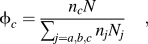 $${\phi _c} = {{{n_c}N} \over {\sum\nolimits_{j = a,b,c} {{n_j}{N_j}} }}\quad ,$$
and the relative A fraction of homopolymers,
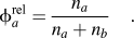 $$\phi _a^{{\rm{rel}}} = {{{n_a}} \over {{n_a} + {n_b}}}\quad .$$
The configuration of the kth polymer of type j is
given by  ${{\underline{R}}_{j,k}}\left( s \right)$, parameterized by
 $s \in \left[ {0,{N_j}} \right]$. We assume that all chains in the system have a Gaussian shape
distribution
 ${\cal P}\left( {{{{\underline{R}}}_{j,k}}\left( s \right)} \right)$. The local monomer densities of A and
B monomers at position
 ${\underline{x}}$ are given by
 ${{\hat \rho }_A}\left( {{\underline{x}}} \right)$ and
 ${{\hat \rho }_B}\left( {{\underline{x}}} \right)$, respectively. The local density
 ${{\hat \rho }_A}\left( {{\underline{x}}} \right) = {{\hat \rho }}_A^{\left( 0 \right)}\left( {{\underline{x}}} \right) + {\hat \rho }_A^{\left( 1 \right)}\left( {{\underline{x}}} \right)$ can be divided into the density
 ${{\hat \rho }}_A^{\left( 0 \right)}\left( {{\underline{x}}} \right)$ from type a homopolymers and the density
 ${\hat \rho }_A^{\left( 1 \right)}\left( {{\underline{x}}} \right)$ from the A part of the copolymers. Analogously,
one has
 ${{\hat \rho }_B}\left( {{\underline{x}}} \right) = {\hat \rho }_B^{\left( 0 \right)}\left( {{\underline{x}}} \right) + {\hat \rho }_B^{\left( 1 \right)}\left( {{\underline{x}}} \right)$. An overview of the notation is given in Fig. 2.
Summary of important parameters and fields. Homopolymers
A and B and copolymers
AB have volume fractions φa, φb, and φc, respectively. Local densities of A monomers
from homopolymers  ${{\hat \rho }}_A^{\left( 0 \right)}$ and copolymer
 ${{\hat \rho }}_A^{\left( 1 \right)}$ sum up to the total local density of
A monomers
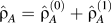 ${{{\hat \rho }}_A} = {{\hat \rho }}_A^{\left( 0 \right)} + {{\hat \rho }}_A^{\left( 1 \right)}$. The notation of B monomer densities is analogous.
In the absence of crosslinks, the partition function of the system can be written as
 $${Z_{nb}} = \prod\limits_{j = a,b,c} {{1 \over {{n_j}!}}\prod\limits_{k = 1}^{{n_j}} {\int {\hat {\cal D}\left\{ {{{{\underline{R}}}_{j,k}}} \right\}{\cal P}\left( {{{{\underline{R}}}_{j,k}}\left( s \right)} \right){\eta _{nb}}\quad ,} } }$$
with path integrals  $\int {\hat {\cal D}\left\{ {{{{\underline{R}}}_{j,k}}} \right\}}$ over all configurations of the kth polymer of
type j and
 $${{\rm{\eta }}_{nb}} \equiv {\rm{\delta }}\left( {{{{\hat \rho }}_A} + {{{\hat \rho }}_B} - {{\rm{\rho }}_0}} \right)\exp \left( { - {1 \over {{{\rm{\rho }}_0}}}\int {dx{\rm{\chi }}{{{\hat \rho }}_A}{{{\hat \rho }}_B}} } \right)\quad .$$
The delta function considers the incompressibility of the system and the exponential term represents the Flory–Huggins interaction with a Flory parameter χ.
Now we consider that reversible crosslinks can form between copolymers. We assume that if a monomer pair A + A, A + B, or B + B is in contact, a crosslink forms with the probability proportional to zωAωA, zωAωB, or zωBωB, respectively (see Fig. 3). One finds that the partition function can then be written as
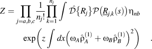 $$Z = \prod\limits_{j = a,b,c} {{1 \over {{n_j}!}}} \prod\limits_{k = 1}^{{n_j}} {\int {\hat {\cal D}\left\{ {{R_j}} \right\}{\cal P}\left( {{{{\underline{R}}}_{j,k}}\left( s \right)} \right){{\rm{\eta }}_{nb}}}}\cr\exp \left( {z\int {dx{{\left( {{{\rm{\omega }}_A}{\hat{\rho }}_A^{\left( 1 \right)} + {{\rm{\omega }}_B}{\hat \rho }_B^{\left( 1 \right)}} \right)}^2}} } \right)} \quad .}$$
Reversible crosslinks can form between copolymers. Crosslinks between two monomers of type X and Y with X, Y ∈ {A, B} form with a probability proportional to zωXωY.
We choose ωA + ωB = 1, so that the crosslink properties are determined by the
crosslink strength and the crosslink asymmetry  $\Delta {\rm{\omega }} \equiv {{\rm{\omega }}_A} - {{\rm{\omega }}_B}$.
In the SCF theory for polymer systems, the Hubbard–Stratonovich (HS)
transformation is used to simplify the expression of the partition function in Eq. (5). Below, we present the
resulting free energy expression with dimensionless quantities, indicated by a
tilde. Dimensionless lengths are defined as  $\tilde x = {x \mathord{\left/ {\vphantom {x {{R_{\rm{g}}}}}} \right. \kern-\nulldelimiterspace} {{R_{\rm{g}}}}}$ with the gyration radius R g of a free
Gaussian polymer of length N. Dimensionless densities are given by
 ${{\tilde \rho }_A} = {{{{\rm{\rho }}_A}} \mathord{\left/ {\vphantom {{{{\rm{\rho }}_A}} {{{\rm{\rho }}_0}}}} \right. \kern-\nulldelimiterspace} {{{\rm{\rho }}_0}}}$, while we use dimensionless free energies of the form
 $\tilde F = {F \mathord{\left/ {\vphantom {F {\left( {{k_B}T{{\rm{\rho }}_0}R_{\rm{g}}^d{N^{ - 1}}} \right)}}} \right. \kern-\nulldelimiterspace} {\left( {{k_B}T{{\rm{\rho }}_0}R_{\rm{g}}^{\,d}{N^{ - 1}}} \right)}}$. Here kT is the thermal energy and
d is the dimension of the system. We use
 ${z_{{\rm{rel}}}} = {{z{{\rm{\rho }}_0}} \mathord{\left/ {\vphantom {{z{{\rm{\rho }}_0}} {\rm{\chi }}}} \right. \kern-\nulldelimiterspace} {\rm{\chi }}}$ for the crosslink strength. With the HS transformation, one
obtains a mean field free energy that can be divided into three termsReference Li, Gruhn and Emmerich25:
 $${\tilde F_{{\rm{tot}}}} = {\tilde F_{\rm{\chi }}} + {\tilde F_{\rm{\omega }}} + {\tilde F_{{\rm{en}}}}\quad .$$
The Flory–Huggins part is given by
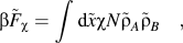 $${\rm{\beta }}{\tilde F_{\rm{\chi }}} = \int {{\rm{d}}\tilde x{\rm{\chi }}N{{{\tilde \rho }}_A}{{{\tilde \rho }}_B}} \quad ,$$
with an inverse thermal energy  ${\rm{\beta }} = {\left( {{k_B}T} \right)^{ - 1}}$. The crosslink contribution can be written as
 $${\rm{\beta }}{\tilde F_{\rm{\omega }}} = \int {{\rm{d}}\tilde x{z_{{\rm{rel}}}}{\rm{\chi }}N{{\left( {{{\rm{\omega }}_A}{\tilde \rho }_A^{\left( 1 \right)} + {{\rm{\omega }}_B}{\tilde \rho }_B^{\left( 1 \right)}} \right)}^2}} \quad .$$
The third term in Eq. (6) considers the entropy of the incompressible polymer blend for given average monomer densities,
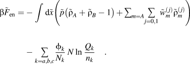 $${\rm{\beta }}{\tilde F_{{\rm{en}}}} = - \int {{\rm{d}}\tilde x\left( {\tilde p\left\big( {{{{\tilde \rho }}_A} + {{{\tilde \rho }}}_B} - 1} \right)\mathop+\sum\limits_{m = A} {\mathop\sum\limits_{j = 0,1} {\tilde w_m^{\left( j \right)}{\tilde \rho }_m^{\left( j \right)}} } } \right)} \cr - \mathop\sum\limits_{k = a,b,c} {{{{\phi _k}} \over {{N_k}}}\,N\ln\, {{{Q_k}} \over {{n_k}}}\quad .} }$$
Here,  $\tilde p\left( {{\underline{x}}} \right)$ stems from the incompressibility condition and
 $\tilde w_X^{\left( j \right)}\left( {{\underline{x}}} \right)$ are auxiliary fields conjugated to the dimensionless equilibrium
densities
 ${\tilde \rho }_X^{\left( j \right)}\left( {{\underline{x}}} \right)$ with X = A,
B and j = 0, 1. Finally, Q k is the partition function of a single polymer chain of type
k fluctuating in the auxiliary fields. A detailed derivation is
given in Ref. Reference Li, Gruhn and Emmerich25.
In the saddle point approximation, variations of the free energy with respect to  $\tilde w_X^{\left( j \right)}\left( {{\underline{x}}} \right)$,
 ${\tilde \rho }_X^{\left( j \right)}\left( {{\underline{x}}} \right)$, and
 $\tilde p\left( {{\underline{x}}} \right)$ must vanish. The resulting equations can be used to calculate
 $\tilde w_X^{\left( j \right)}\left( {{\underline{x}}} \right)$,
 ${\tilde \rho }_X^{\left( j \right)}\left( {{\underline{x}}} \right)$, and
 $\tilde p\left( {{\underline{x}}} \right)$ numerically. An algorithm is described in Ref. Reference Li, Gruhn and Emmerich25.
III. PHASE DIAGRAM
The theoretical model, described in the previous section, has been used for a
comprehensive study of symmetric AB + A
+ B polymer blends with reversibly crosslinking
copolymers. We consider homopolymers of lengths  ${N_a} = {N_b} = {N \mathord{\left/ {\vphantom {N 5}} \right. \kern-\nulldelimiterspace} 5}$, where N ≡ N c is the length of the copolymers. For the sake of a reasonable computational
effort, we restrict the calculations to two-dimensional systems with box lengths
L x and L y and an area
 $A = {L_x}{L_y}$. We use periodic boundary conditions, a Flory parameter of
χN = 11.3 and a volume fraction
 ${\phi _c} = 0.6$ of copolymers. For calculating the single-polymer partition
functions, concentration fields, and auxiliary fields, we use a discretization on a
square grid in real space. In future calculations, Fourier mode methods may be used
to speed up the calculations.
The phase diagram has been studied in the range of  $0.5 \le \phi _A^{{\rm{rel}}} \le 0.75$,
 $0 \le {z_{{\rm{rel}}}} \le 2$, and
 $- 1 \le \Delta {\rm{\omega }} \le 1$. Depending on these parameters, the system formed two different
phases in the observed phase region, a hexagonal phase for small
z rel and
 $\left| {\Delta {\rm{\omega }}} \right|$ as well as a lamellar phase for suitably large
z rel and
 $\left| {\Delta {\rm{\omega }}} \right|$. As shown below, the transition between these two phases is of
first order. Close to the phase boundaries, there are strong hysteresis effects and
the structure found in the calculations depends on the start configuration. To
overcome this problem, we study small systems with a box length ratio of
 ${{{L_y}} \mathord{\left/ {\vphantom {{{L_y}} {{L_x}}}} \right. \kern-\nulldelimiterspace} {{L_x}}} = \sqrt 3$. In this geometry, unit cells of the hexagonal or the lamellar
phase can form if L x is of the correct size. We have varied L x in the range of
 $3.0 \le {L_x} \le 4.8$. The number of grid points was kept fixed. Frequently, we tested
that discretization effects are negligible by comparing calculations with different
grid sizes up to systems with 960 ✕ 1663 grid points. From the lowest
free energy obtained in the interval
 $3.0 \le {L_x} \le 4.8$, we determine the stable phase. Figure 4(a) shows a sequence of free energy plots for
 $\phi _a^{{\rm{rel}}} = 0.65$,
 $\Delta {\rm{\omega }} = 0.2$, and various values of z. The phase transition
occurs at
 ${z_{{\rm{rel}}}} \simeq 0.8$. The density of A monomers is shown for a
lamellar phase in Fig. 4(b) and for a
hexagonal phase in Fig. 4(c).
(a) Free energy of the system as a function of box length L x with  ${{{L_y}} \mathord{\left/ {\vphantom {{{L_y}} {{L_x}}}} \right. \kern-\nulldelimiterspace} {{L_x}}} = \sqrt 3$,
 $\phi _a^{{\rm{rel}}} = 0.65$,
 $\Delta {\rm{\omega }} = 0.2$, and different values of z. Empty
circles correspond to the lamellar phase [see unit cell in (b)], filled
boxes correspond to the hexagonal phase [see unit cell in (c)]. The
dotted lines help to see the differences between the local energy minima
of the hexagonal and the lamellar phases.
With the described method, we have calculated the phase diagram as a function of  $\phi _a^{{\rm{rel}}}$, z rel, and Δω.
The result is depicted in Fig. 5. It shows
phase boundaries between the hexagonal and the lamellar phase for different values
of
 $\phi _a^{{\rm{rel}}}$. Note that for symmetry reasons, it is sufficient to study
 $\phi _a^{{\rm{rel}}} \ge 0.5$. For
 $\phi _a^{{\rm{rel}}} \ge 0.58$, the system shows a hexagonal phase for suitably small
z and
 $\left| {\Delta {\rm{\omega }}} \right|$ separated by the phase boundaries from the lamellar phase outside.
The phase diagram is not symmetric with respect to ∆ω
= 0 or any other horizontal line ∆ω =
constant. The asymmetry is caused by the excess of A homopolymers
for
 $\phi _a^{{\rm{rel}}} \ge 0.5$.
Phase diagram of the AB + A
+ B polymer blend: The colored curves denote
the phase boundaries between the hexagonal phase on the inside (small  $\left| {\Delta \omega } \right|$) and the lamellar phase on the outside. Phase
boundaries are shown for
 ${\phi _A} = 0.75$ (dark blue),
 ${\phi _A} = 0.7$ (red),
 ${\phi _A} = 0.65$ (green),
 ${\phi _A} = 0.6$ (brown),
 ${\phi _A} = 0.59$ (magenta), and
 ${\phi _A} = 0.58$ (cyan).
The hexagonal phase region expands with increasing  $\phi _a^{{\rm{rel}}}$. For values
 $\phi _a^{{\rm{rel}}} \ge 0.57$, only lamellar phases have been found for
z rel > 0. For
z rel = 0, the system always forms a hexagonal
phase.
IV. COMPARISON OF FREE ENERGY CONTRIBUTIONS IN THE HEXAGONAL AND THE LAMELLAR PHASE
Analyzing the density distributions of the lamellar and the hexagonal phase, we have
found that the system forms more pronounced oscillations of  ${\rm{\rho }}_A^{\left( 1 \right)}$ and
 ${\rm{\rho }}_B^{\left( 1 \right)}$ in the lamellar phase than in the hexagonal phase. The stronger
oscillations in the lamellar phase leads to a more negative crosslink contribution
to the free energy,
 $\tilde F_{\rm{\omega }}^{{\rm{lam}}} \lt \tilde F_{\rm{\omega }}^{{\rm{hex}}}$. Figure 6 shows the
differences
 $\Delta \tilde F = {\tilde F^{{\rm{hex}}}} - {\tilde F^{{\rm{lam}}}}$ between the hexagonal and the lamellar phase for a system with
 $\phi _a^{{\rm{rel}}} = 0.65$, ∆ω = 0.2, and various
z. For the same systems, free energies
 ${\tilde F_{{\rm{tot}}}}\left( {{L_z}} \right)$ are shown in Fig. 4(a).
The total free energy  ${\tilde F_{{\rm{tot}}}}$ consists of a crosslink part
 ${\tilde F_{\rm{\omega }}}$, a Flory–Huggins part
 ${\tilde F_{\rm{\chi }}}$, and an entropy part
 ${\tilde F_{{\rm{en}}}}$ [see Eq.
(6)]. For suitably large crosslink strength
z rel, the crosslink free energy
 $F_{\rm{\omega }}^{{\rm{hex}}}$ in the hexagonal phase is distinctly larger than
 $F_{\rm{\omega }}^{{\rm{lam}}}$ in the corresponding lamellar phase so that the
difference
 $\Delta {\tilde F_{\rm{\omega }}} = \tilde F_{\rm{\omega }}^{{\rm{hex}}} - \tilde F_{\rm{\omega }}^{{\rm{lam}}}$ is distinctly larger than zero. For
 ${z_{{\rm{rel}}}} > 0.8$, this stabilization of the lamellar phase wins over
the remaining free energy contributions
 ${\tilde F_{{\rm{en}}}} + {\tilde F_{\rm{\chi }}}$ that favor the hexagonal phase (note that
 $\Delta {\tilde F_{{\rm{en}}}} + \Delta {\tilde F_{\rm{\chi }}} = \left( {\tilde F_{{\rm{en}}}^{{\rm{hex}}} - \tilde F_{{\rm{en}}}^{{\rm{lam}}}} \right) + \left( {\tilde F_{\rm{\chi }}^{{\rm{hex}}} + F_{\rm{\chi }}^{{\rm{lam}}}} \right) \lt 0$). In the inset,
 $\Delta {\tilde F_{{\rm{en}}}}$ and
 $\Delta \tilde F{\rm{\chi }}$ are shown, separately. Free energy values are taken
from corresponding hexagonal and lamellar phases at the respective local
minima of
 ${\tilde F_{{\rm{tot}}}}$, which are shown in Fig. 4(a) for
 $\phi _a^{{\rm{rel}}} = 0.65$,
 $\Delta {\rm{\omega }} = 0.2$, and different values of z. See Sec.
IV for a discussion of the free energy contributions.
The difference  $\Delta {\tilde F_{\rm{\omega }}} = \tilde F_{\rm{\omega }}^{{\rm{hex}}} - \tilde F_{\rm{\omega }}^{{\rm{lam}}}$ between the free energy contributions from the crosslinks is
positive for all values of z. The sum of the remaining free energy
contributions is always lower in the hexagonal phase
 $\left( {\Delta {{\tilde F}_{{\rm{en}}}} + \Delta {{\tilde F}_{\rm{\chi }}} \lt 0} \right)$. In the inset of Fig. 6,
 $\Delta {\tilde F_{{\rm{en}}}}$ and
 $\Delta {\tilde F_{\rm{\chi }}}$ are shown, individually. The absolute value of both quantities is
much larger than that of ΔF tot, but
 $\Delta {\tilde F_{{\rm{en}}}}$ and
 $\Delta {\tilde F_{\rm{\chi }}}$ have opposite signs and their sum is of the order of
ΔF tot. The value
 $\Delta {\tilde F_{{\rm{en}}}}$ decreases with increasing z rel,
whereas
 $\Delta {\tilde F_{\rm{\chi }}}$ gets larger. For
 ${z_{{\rm{rel}}}} \ge 0.4$, the entropy is larger in the hexagonal state, whereas the
Flory–Huggins contribution is more pronounced in the lamellar phase. For
a stabile hexagonal phase, the difference between the volume fractions of
homopolymers A and B must be suitably large, i.e.,
 $\phi _a^{{\rm{rel}}}$ must be big enough. Then, the entropic free energy contribution
 $\Delta {\tilde F_{{\rm{en}}}}$ profits from the hexagonal structure, in which the circular
domains are predominantly filled with B monomers. For larger
z rel or Δω, the crosslink
contribution dominates. Studying the density distribution in the lamellar phase, one
finds that
 ${\tilde \rho }_A^{\left( 1 \right)}$ and
 ${\tilde \rho }_B^{\left( 1 \right)}$ oscillates almost symmetrically around
 ${{\tilde \rho }^{\left( 1 \right)}}$.
With  $\Delta {{\tilde \rho }^{\left( 1 \right)}} \equiv {\tilde \rho }_A^{\left( 1 \right)} - {\tilde \rho }_B^{\left( 1 \right)}$ the free energy contribution
 ${\tilde F_{\rm{\omega }}}$ can be written as
 $$ & \tilde F_{\rm{\omega }} = - z\int {{\rm{d}}\tilde x\left( {{{1 + \Delta {\rm{\omega }}} \over 2}\left( {{\rm{\rho }}^{\left( 1 \right)} + \Delta {\rm{\rho }}^{\left( 1 \right)} } \right) \cr + {{1 + \Delta {\rm{\omega }}} \over 2}\left( {{\rm{\rho }}^{\left( 1 \right)} - \Delta {\rm{\rho }}^{\left( 1 \right)} } \right)} \right)^2 } \cr & \quad \, \simeq -{z \over 4}\int {{\rm{d}}\tilde x\left( {\left( {{{\tilde \rho }}^{\left( 1 \right)} } \right)^2 + \Delta {\rm{\omega }}^2 \left( {\Delta {{\tilde \rho }}^{\left( 1 \right)} } \right)^2 } \right)} \quad . \cr} $$
For a given lamellar density distribution,  ${\tilde F_{\rm{\omega }}}$ decreases with increasing z or
 $\left| {\Delta {\rm{\omega }}} \right|$, independent of the sign of Δω. Thus, a
demixing of the A and B parts of the copolymers is
more favored as z or
 $\left| {\Delta {\rm{\omega }}} \right|$ increases.
It is interesting to compare the phase behavior of our system with that of regular
copolymer blends. For the latter systems, the large values of the parameter
Nχ/T support a higher degree of
order and segregation in the system and counteracts the mixing tendency of the
entropy.Reference Helfand29–Reference Hillmyer, Maurer, Lodge, Bates and Almdal32 For our system with reversible
crosslinks, large values of χ, z, and  $\left| {\Delta {\rm{\omega }}} \right|$ support a higher degree of order. With this respect, we find that,
similar to regular copolymer blends,Reference Helfand29–Reference Hillmyer, Maurer, Lodge, Bates and Almdal32 the
lamellar phase is more stable than the hexagonal phase if a high degree of order is
favored.
However, phase stability depends sensitively on details of the polymer blend. In our
system, an excess of A homopolymers  $\left( {\phi _A^{{\rm{rel}}} > 0.5} \right)$ supports the hexagonal phase, in which the A-rich domains are
larger than the circular B-rich domains; the size of the hexagonal part of the phase
diagram grows with increasing
 $\phi _A^{{\rm{rel}}}$. One might expect the same effect in systems of noncrosslinking
block copolymers if the length l A is larger than the length l B of the B blocks. Such systems have been studied with the SCF theory.Reference Matsen and Bates34 It was found that for a small excess of A monomers, the
hexagonal phase is most stable. However, for distinctly longer A
blocks
 $\left( {{{{l_A}} \mathord{\left/ {\vphantom {{{l_A}} {{l_B}}}} \right. \kern-\nulldelimiterspace} {{l_B}}} \mathbin{\gsim\lower.3ex\hbox{$\buildrel\over {\smash{\scriptstyle}\vphantom{_x}}$}} 0.68} \right)$, the lamellar phase is more stable than the hexagonal phase. (In
addition, these systems form three-dimensional microphases. For details, we refer to
Ref. Reference Matsen and Bates34.)
V. CONCLUSIONS
An extended SCF theory has been used to investigate a polymer blend formed by
AB diblock copolymers and A and
B homopolymers. Reversible crosslinks are considered between the
copolymers with a crosslink strength z and a crosslink asymmetry
∆ω = ωA − ωB. We obtain a phase diagram as a function of  $\phi _a^{{\rm{rel}}} > 0.5$, z rel, and Δω.
For
 $\phi _a^{{\rm{rel}}} \lt 0.58$ and z rel > 0, only a lamellar
phase is found. Otherwise, a hexagonal phase is found for suitably small
z rel and
 $\left| {\Delta {\rm{\omega }}} \right|$. With increasing
 $\phi _a^{{\rm{rel}}}$, the stoichiometry gets more asymmetric, and the asymmetric
hexagonal phase region in the phase diagram grows.
Our studies reveal that the structure of the studied system can be switched from the
hexagonal phase to the lamellar phase and back by changing the crosslink properties
or the stoichiometry of the system. The first switching method can be achieved with
crosslinks that depend on external parameters like the temperatureReference Adelsberger, Metwalli, Diethert, Grillo, Bivigou-Koumba, Laschewsky, Müller-Buschbaum and Papadakis33 or illumination.Reference Huck35 The second switching method can be easily achieved by changing the ratio
between the volume fractions of A and B
homopolymers. Analyzing the free energy contributions for  $\phi _a^{{\rm{rel}}} \ge 0.58$, we find that the hexagonal phase has a larger entropic
contribution to free energy, whereas the crosslink free energy contribution is
stronger in the lamellar phase.
With these studies, we have shown that our extended version of the SCF theory is an excellent tool for a detailed investigation of reversibly crosslinked polymer networks. Many advanced SCF techniques, developed for complex polymer blends without crosslinks, can be combined with our method to study reversibly crosslinked polymer networks with more complex structures.
ACKNOWLEDGMENT
This work was supported by DFG SPP 1259: “Intelligente Hydrogele, modeling and simulation of hydrogel swelling under strong non-equilibrium conditions using the phase-field and phase-field crystal methods” and by DFG SFB 840: “Von Partikulären Nanosystemen zur Mesotechnologie.”



