Emission taxes when pollution depends on location

Walid Marrouch; Bernard Sinclair-Desgagné

doi:10.1017/S1355770X12000101

Emission taxes when pollution depends on location

Published online by Cambridge University Press: 09 March 2012

Walid Marrouch and

Bernard Sinclair-Desgagné

Show author details

Walid Marrouch: Affiliation:
School of Business, Lebanese American University, Lebanon; and CIRANO. Email: walid.marrouch@lau.edu.lb
Bernard Sinclair-Desgagné: Affiliation:
HEC Montréal, 3000 Chemin de la Côte-Sainte-Catherine, Montréal (Québec), Canada H3T 2A7; CIRANO and École Polytechnique de Paris. Email: bsd@hec.ca

Article contents

Abstract
Introduction
The model
First case: polluters are price-takers
Second case: polluters form a monopoly
Concluding remarks
Footnotes
References

Rights & Permissions

Abstract

It is well known that an efficient pollution taxation scheme should charge each source according to its specific marginal contribution to social damages. Despite significant advances in environmental assessment, geographic information systems and data analysis, this requirement would impose technical, informational and administrative expenses that most regulators – notably in developing countries – seem unable to afford. This paper shows that it can actually be less demanding than it seems. If polluters are price-takers, for instance, in a context where the affected population concentrates at a given location, then the optimal emission tax will disregard a source's location. Otherwise, the adjustment of the optimal tax to location will depend on the extent of a polluter's market power.

Information

Type: Theory and Applications
Information: Environment and Development Economics , Volume 17 , Issue 4 , August 2012 , pp. 433 - 443

DOI: https://doi.org/10.1017/S1355770X12000101 [Opens in a new window]
Copyright: Copyright © Cambridge University Press 2012

1. Introduction

To the extent that the social costs associated with certain polluting activities often depend on the geographic area where such activities are taking place, one reasonably expects optimal corrective measures to take spatial information into account. Indeed, Tietenberg (Reference Tietenberg1974), Henderson (Reference Henderson1977), Hochman et al. (Reference Hochman, Pines and Zilberman1977), Hochman and Ofek (Reference Hochman and Ofek1979), Baumol and Oates (Reference Baumol and Oates1988), and others have emphasized early on that policy instruments, notably taxes, should explicitly consider local features that influence the amount and impact of polluting emissions. Over the past 30 years, a number of studies in the fields of urban/regional and environmental economics have also pursued this line of investigation.Footnote ¹ Some theoretical contributions, such as Xepapadeas (Reference Xepapadeas1992) and Uimonen (Reference Uimonen2001), sought to develop sophisticated price instruments. Applied works, on the other hand, often built on novel technologies, such as Geographic Information Systems (GIS), which are now helping environmental economists to collect and use spatial data.Footnote ²

A major practical limitation of fine-tuned environmental policies, however, has traditionally been the technical and administrative costs involved in gathering and processing the needed information.Footnote ³ In a recent paper, Muller and Mendelsohn (Reference Muller and Mendelsohn2009: 1735) yet argue that ‘… calculating the marginal damages of emissions for a large number of air pollution sources is [now] possible and practical, [so …] regulations can now move from cost effectiveness to efficiency [and …] incorporate source-specific marginal damages of emissions into policy’. They illustrate this in a convincing fashion by cleverly using a well-established integrated assessment model which tracks the consequences of several regulated air pollutants – coarse particulate matter, sulfur dioxide, fine particulate matter, volatile organic compound and ammonia – to impute the resulting damages to 10,000 separate sources across the United States. The welfare gains from updating current policies based on this information are shown to be quite substantial. But whether the same exercise can be performed equally well in other countries and for other types of pollution remains to be seen. In the context of riverbed downstream sedimentation caused by upstream farming activities, for example, which is a common environmental problem adversely affecting users of watersheds, notably in developing countries,Footnote ⁴ governments are a priori likely to still lack the necessary expertise, technology and administrative resources to collect and use geographic information effectively.

This paper's raison d'être is to point out that the role of geographical information in crafting a pollution taxation scheme depends anyhow on the polluters' market power. If, in particular, polluting firms have no market power, then an efficient tax might be set which economizes on locational data. In a nutshell, market intelligence modulates, and might sometimes substitute for, spatial information.

The literature on spatial taxation has so far ignored the additional distortions induced by imperfect competition. This paper contributes an analysis à la Buchanan (Reference Buchanan1969) and Barnett (Reference Barnett1980), whereby two polar market structures – perfect competition and monopoly – are being considered; the optimal tax rule is then shown to ignore geography in the former case but to tradeoff spatial adjustments and market power in the latter. These results rest on a specific context, however. Unlike Muller and Mendelsohn (Reference Muller and Mendelsohn2009), we assume that all pollutees lie at a single point in a stylized landscape and that the positive (output) and negative (emissions) contributions from a given source depend on distance from this point only.Footnote ⁵ This framework applies to situations such as noise, smells, light or other similar nuisances, where the major disamenity is caused by the level/quantity of the pollutant reaching the pollutee. Such location-dependent environmental externalities are pervasive in both rural and urban settings. Man-made silt build-up in riverbeds provides another stylized case of particular interest.Footnote ⁶ Around the world, hundreds of rivers are currently dammed, among which 37 are major ones, and 261 rivers make up several internationally shared basins.Footnote ⁷ One then often sees a river with a downstream reservoir serving a nearby city in transportation, water and/or hydroelectricity while some homogeneous farming activities are taking place upstream. Through land clearing and excavation, farming causes soil erosion, thereby accelerating the sedimentation of downstream basins. This can entail substantial social damages. Reporting on some studies of the Panama Canal, for instance, The Economist magazine asserted that:Footnote ⁸

Deforestation allows more sediment and nutrients to flow into the canal. Sediment clogs the channel directly. Nutrients do so indirectly, by stimulating the growth of waterweeds. Both phenomena require regular, and expensive, dredging.

Silt build-up in reservoirs also makes electricity generation more costly and reduces both the quantity and quality of water.

This paper will now unfold as follows. The upcoming section lays out the model. Section 3 considers the situation where polluters are price-takers. Section 4 deals with the monopolistic polluter case. Section 5 makes concluding remarks.

2. The model

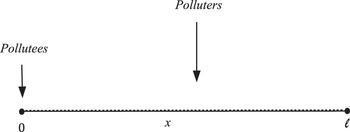
Consider the stylized landscape pictured in figure 1. It is composed of a continuum of identical polluters uniformly distributed on a line of total length ℓ, and some affected party (the pollutees) situated at the extreme left-hand side. The latter location, which we associate with that of a city/urban center or marketplace, is labeled as the origin (0). The variable x thus denotes the distance between polluters and pollutees.

Figure 1.

The landscape.

In this model, the magnitude of the externality caused by a specific polluter will only depend on the latter's location x. This stylized assumption seems to match the specific but quite frequent situations mentioned in the introduction, such as the soil erosion and sedimentation provoked by farming activities occurring upstream along a river that feeds a city's water reservoir.Footnote ⁹

2.1. The polluters

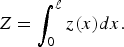
Assume all polluters deliver a homogeneous product, and let z(x) denote the output of a polluting firm/farm/individual (thereafter referred to as a source) situated at x. Total production is thus given by

(1)

$Z = \vint_0^{\ell} z\lpar x\rpar dx.$

At output level z(x), the corresponding polluter incurs a cost C(z, x) which depends on its distance x from the market. This cost function is strictly increasing and convex in both z and x, and the cross derivative C _zx is strictly positive. Convexity in the distance x, and the assumption that the marginal cost of production increases in x, can mean that polluters located farther from the market suffer larger transportation and marketing costs.

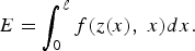
Suppose that a source's emissions are captured by the function f(z, x) which is increasing and convex in z. This reflects the fact that pollution grows at an increasing rate with production. On the other hand, let f _x < 0 and f _zx < 0. The latter indicate that, all things equal, external damages are less important when the source is more distant from the city. To keep things tractable, we assume that a source's pollution does not affect other polluters' production. The overall level of pollution is thus given by

(2)

$E = \vint_0^{\ell} f\lpar z\lpar x\rpar \comma \; x\rpar dx.$

Let us now turn to the affected party.

2.2. The consumers

People located at the origin will consume the overall output Z; let p(Z), with p′(Z) < 0, denote their aggregated inverse demand for the product, where Z is given by (1). They also endure a disamenity a(E) which increases linearly with total emissions, i.e., a = ν E with some positive coefficient ν.

A non-indexed coefficient ν means of course that we are considering here a representative pollutee. This assumption can be justified by the fact that pollutees are located at a single node in our framework. The heterogeneity of the firms/polluters, on the other hand, is embedded in the total emissions function defined in (2), which depends on how a firm's specific location affects its pollution.

Note also that making the disamenity depend on concentration rather than total emissions would not qualitatively change our results. In this static model, the stock or concentration of pollutants could be given by any function of total emissions S = S(E) with S′(E) > 0. The disamenity suffered at the city node might then alternatively amount to a = a(S) where a′(S) > 0. In this case, we have that 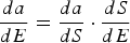$\displaystyle{{da} \over {dE}} = \displaystyle{{da} \over {dS}} \cdot \displaystyle{{dS} \over {dE}}$ using the chain rule. The relationship between a and S is then implicit in the functional form a = ν E through the coefficient ν.

We shall now compute the optimal emission tax in this setup, assuming at first that polluters are price-takers.

3. First case: polluters are price-takers

In the absence of a tax on polluting emissions, each price-taking polluter maximizes profits

$\pi \lpar z\rpar = pz - C\lpar z\comma \; x\rpar \comma \;$

so its marginal cost matches the market price

$p\lpar {\bi Z}\rpar = C_z \lpar z\comma \; x\rpar .$

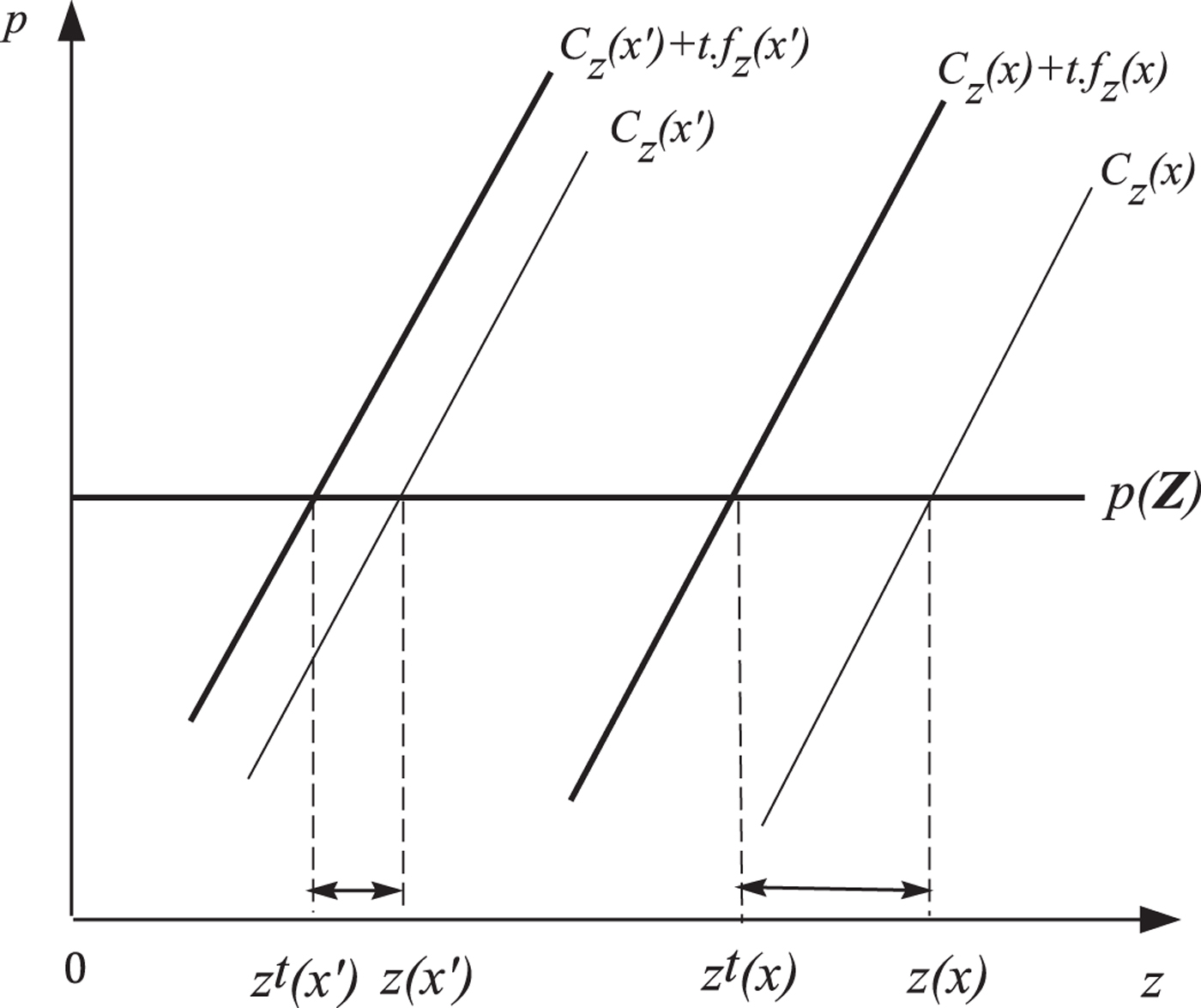
Since this marginal cost increases with the distance x from the market (recall that C _zx > 0), a more remote source delivers less output. It follows that the derivative z _x < 0. This situation is depicted in figure 2 (assuming a quadratic cost function).

Figure 2.

The effect of location and taxation on marginal costs (x′ > x).

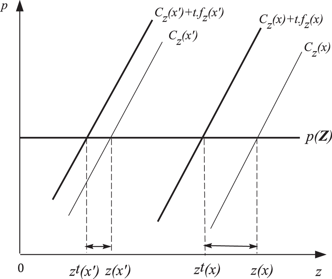
Suppose a positive tax t per unit of pollution/disamenity is imposed. A polluter situated at x will maximize the profit function

$\pi \lpar z\rpar = pz-C\lpar z\comma \; x\rpar - t\cdot f\lpar z\comma \; x\rpar \comma \;$

thereby setting a production level that satisfies the first-order condition

(3)

$p\lpar {\bi Z}\rpar = C_z + t\cdot f_z.$

Meeting (3) entails of course that the output goes down as t goes up.

Let now the corrective tax be set by a benevolent regulator who seeks the largest value of the sum of consumer surplus and producer benefits minus the social disamenity. Ignoring redistribution and income transfer issues, and replacing E by the right-hand-side formula in (2), the tax should then maximize

(4)

$W = \vint_0^{{\bi Z}^t} p\lpar u\rpar du - \vint_0^{\ell} C\lpar z^t\comma \; x\rpar dx - \nu \vint_0^{\ell} f\lpar z^t\comma \; x\rpar dx\comma \;$

where the superscript t in (4) refers to the polluters' adjusted output once they bear the tax. The necessary and sufficient first-order condition for an optimal policy is now

(5)

$W^\prime\lpar t\rpar = \vint_0^{\ell} \left(p\lpar {\bi Z}\rpar \displaystyle{{dz} \over {dt}} - C_z \displaystyle{{dz} \over {dt}} - \nu f_z \displaystyle{{dz} \over {dt}}\right)dx = 0.$

Condition (5) holds only when

(6)

$p\lpar {\bi Z}\rpar \displaystyle{{dz} \over {dt}} - C_z \displaystyle{{dz} \over {dt}} - \nu f_z \displaystyle{{dz} \over {dt}} = 0$

is true at every point (x) ∈ [0, ℓ].Footnote ¹⁰ Substituting (3) into (6) yields the following expression for an optimal emission tax:

(7)

$t = \nu.$

This is precisely the original Pigouvian tax (Pigou Reference Pigou1920), which equals the (in the present setting, location-invariant) marginal social disamenity.

Proposition 1

When polluters have no market power, the optimal pollution tax is the standard Pigouvian one, t = ν, which ignores spatial information.

This result might suggest that there is no difference between our setup and the standard one where polluters are taxed regardless of their location-dependent impact. Note, however, that while the above tax given by (7) is uniform across locations, polluters will adjust according to their specific production spot. To see this, recall from expression (3) that

$p\lpar {\bi Z}\rpar = C_z \lpar z\comma \; x\rpar + t \cdot f_z \lpar z\comma \; x\rpar .$

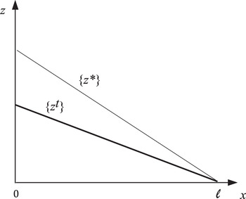
Since the marginal contribution to pollution f _z decreases in x, a more distant (hence less polluting and productive) source needs therefore to adjust proportionally less than one that is located closer to the market (see figure 2). Thus, as figure 3 illustrates, this corrective measure's final outcome is to render the distribution of production across space z(x) flatter.Footnote ¹¹

Figure 3.

The effect of taxation on production distribution.

The difference between our framework and the standard one will nonetheless be more striking in the next section, as we address a case in which polluters have market power.

4. Second case: polluters form a monopoly

Suppose that all producers in the present landscape collude to form a monopoly.Footnote ¹² Their common objective is then to maximize their joint profits

$\Pi\lpar {\bi Z}\rpar = p\lpar {\bi Z}\rpar {\bi Z} - \vint_0^{\ell} C\lpar z\comma \; x\rpar dx - t\vint_0^{\ell} f\lpar z\comma \; x\rpar dx.$

Therefore, the production level at every spot x must altogether satisfy the following first-order condition

(8)

$\vint_0^{\ell} \lsqb p^{\prime}\lpar {\bi Z}\rpar z + p\lpar {\bi Z}\rpar - C_z -tf_z\rsqb dx = 0.$

Condition (8) indicates that

(9)

$p^{\prime}\lpar {\bi Z}\rpar z + p\lpar {\bi Z}\rpar - C_z -tf_z = 0$

at every x ∈ [0, ℓ].Footnote ¹³ Substituting (9) into (6) yields the general formula for the optimal tax per unit of polluting emission:

(10)

$t\lpar x\rpar = \nu + \displaystyle{p^{\prime}\lpar {\bi Z}\rpar z\displaystyle{{dz} \over {dt}} \over f_z \displaystyle{{dz} \over {dt}}}.$

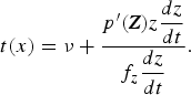
The second term on the right-hand side is negative, so the new tax rate is actually smaller than the one proposed in the previous section. This agrees with the classical results of Buchanan (Reference Buchanan1969) and Barnett (Reference Barnett1980). The underlying intuition is now well known: in the presence of a monopolistic polluter, the optimal corrective tax must be set lower than the marginal social cost of damage in order to alleviate the consequent strategic reduction in output. Expression (10) can in fact be rewritten as

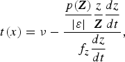
$t\lpar x\rpar = \nu - \displaystyle{\displaystyle{p\lpar {\bi Z}\rpar \over \vert \varepsilon\vert } \displaystyle{z \over {\bi Z}} \displaystyle{dz \over dt} \over f_z \displaystyle{dz \over dt}}\comma \;$

where ɛ denotes the price-elasticity of demand. As demand becomes less elastic, the size of the downward adjustment tends therefore to increase. This property limits the exercise of market power by the monopolist and prevents consumer surplus from falling too drastically.

This taxation scheme also presents an original feature: its downward adjustment term takes into account the respective impacts of each source according to its specific location. Comparative statics with respect to the spatial coordinate x implies indeed that

(11)

$\displaystyle{\partial t \over \partial x} = p^{\prime}\lpar {\bi Z}\rpar \left(\displaystyle{z_x \lpar f_z -zf_{zz}\rpar - zf_{zx} \over \lpar f_z\rpar ^2}\right).$

The sign of (11) now depends on that of A = z _x(f _z–zf _zz–zf _zx. Straightforward manipulations reveal that

(12)

$A \lesseqgtr 0 \Leftrightarrow \displaystyle{{z_x } \over {z}}\lpar 1-\eta\rpar \lesseqgtr \displaystyle{{f_{zx}} \over {f_z}}\Leftrightarrow \displaystyle{{\partial t} \over {\partial x}} \gtreqless 0$

where $\eta =\displaystyle{f_{zz} \over f_{z}}z$ is the elasticity of a polluter's marginal contribution to pollution with respect to output z. This yields the following proposition.

Proposition 2

If all polluting sources operate altogether as a monopoly, the optimal emission tax increases (decreases) with the spatial coordinate x if and only if the adjusted rate of change of output relative to location, given by $\displaystyle{z_x \over z}\lpar 1 - \eta\rpar$ , is smaller (larger) than the rate of change of the marginal contribution to pollution with respect to location $\left(\displaystyle{f_{zx} \over f_z}\right)$ .Footnote ¹⁴

The elasticity coefficient η spans in fact two distinct intervals. In the higher range where η > 1, the marginal contribution to pollution is very responsive to output. We have from (12) that

$\displaystyle{z_x \over z}\lpar 1 - \eta\rpar \gt \displaystyle{f_{zx} \over f_z} \Leftrightarrow \displaystyle{\partial t \over \partial x} \lt 0\comma \;$

so the optimal pollution tax must decrease in the distance x unambiguously. In the inelastic range where 0 < η< 1, i.e., when the marginal contribution to pollution is not too responsive to an increase in output, on the other hand, the tradeoff highlighted in our proposition holds. If output z(x) drops by a larger amount than the marginal contribution to pollution for a given increase in the distance x from the urban center/market, then the optimal pollution tax is set to augment with x. In this case, the tax rule provides reduced incentives for the monopoly to shift production from closer sources to farther ones, where larger production costs will translate into higher prices for consumers with relatively little compensation on the environmental side. The opposite occurs when the marginal contribution to pollution drops by a larger amount than production as x increases: the optimal tax is set to decrease with the distance x, for the positive impact on welfare of shifting production away from the urban center/market outweighs the negative impact this has on consumer prices.

5. Concluding remarks

We studied an emission tax scheme meant to regulate polluting activities when their impact on a given pollutee is inversely related to distance. The upshot is that this remedy should be location dependent only when polluters have some market power. In this case, it should be proportional to the marginal social cost of pollution and also depend on observables such as local productivity and distance from the affected party.

As we pointed out initially, our model seems to fit several concrete situations, notably in developing countries, such as the pollution of a river, riverway or canal – due to recurrent agricultural activities taking place along its banks – which affects the inhabitants of a downstream city. Implementing the above taxation scheme in these contexts will of course require further refinements. Dealing with other market structures, such as monopolistic competition, is perhaps the most obvious one. Land rents and farm location should also be made endogenous.

Although we focused here on taxes, our analysis may contain suggestions for other types of instruments, such as zoning. Zoning can of course take various forms: it may consist of a complete ban on all farming activities, for instance, or it may just require farmers to offset erosion by planting trees and other soil-preserving plants in specific areas. All things considered, when farmers have some market power a tradeoff similar to the one outlined in proposition 2 would make it preferable to create a buffer zone free of farming activities near the riverbank or waterway.

Further extended, the above conclusions may also inform the current discussions on ‘eco-conditionality’, or whether and how much to reward farmers for their ‘environmental services’ (such as safeguarding the beauty of certain rural areas and sheltering endangered species). To see this, note that the above tax t and environmental cost ν could be assumed negative; they would then correspond respectively to a subsidy and an environmental amenity enjoyed by urban citizens (which becomes smaller as it is generated farther away). If farmers collude (forming a cooperative or some powerful association), then proposition 2 recommends to base individual grants, not only on the marginal value of the provided environmental services, but also on distance and local productivity.

Finally, the generic question raised at the beginning of this paper – what type of information does the regulator need to learn? – is of significant practical use, especially in developing countries where governments have limited means. Although there is a vast literature on environmental policy under asymmetric information, few articles have so far addressed this precise issue (a paper by Magesan and Turner (Reference Magesan and Turner2010) is a notable recent exception). In the specific case where closer polluters inflict greater damages to a given pollutee, we showed that market intelligence can often substitute for geographical information. Whether and how similar assertions can be made in other contexts awaits further investigation.

Footnotes

¹ For an excellent review on spatial land use, see Bockstael and Irwin (Reference Bockstael, Irwin, Folmer and Tietenberg2000) and Hardie et al. (Reference Hardie, Parks, van Kooten, Folmer and Tietenberg2004). Works drawing instead on Hotelling's (Reference Hotelling1929) seminal linear-city model are also carefully surveyed by Gerking and List (Reference Gerking, List, Folmer, Gabel, Gerking and Rose2001) and Geoghegan and Gray (Reference Geoghegan, Gray, Folmer and Tietenberg2005).

² Bateman et al. (Reference Bateman, Yang, Boxall, Folmer and Tietenberg2006) provide a good survey of GIS applications.

³ See Laffont and Tirole (Reference Laffont and Tirole1993, chapter 1) for further discussion of administrative regulatory costs.

⁴ Bockstael and Irwin (Reference Bockstael, Irwin, Folmer and Tietenberg2000) offer a good discussion of the soil erosion problems caused by farming.

⁵ This means that polluters use similar production and abatement technologies. It also excludes uniformly mixed pollutants such as greenhouse gases, whose contribution to environmental depletion does not depend on location.

⁶ Noise, light, odors and silt are typical examples of local pollutants. In some cases – when polluters and pollutees reside in different countries – they will also generate international conflicts. Moreover, they might soon become a topic of global concern, because of their impact on habitats, ecosystems and biodiversity (Hogan et al., Reference Hogan, Caley, McGinley and Cleveland2010). Dealing with transboundary pollution or global environmental issues, however, is beyond the scope of this article.

⁷ For further information, see ‘International river basins of the world’ in the Transboundary Freshwater Dispute Database, available at http://www.transboundarywaters.orst.edu/.

⁸ See ‘Environmental economics, are you being served?’, in The Economist, print edition, 21 April 2005.

⁹ An interesting alternative would be to have production occurring at a point and polluting consumers dispersed along a line (say, the production point is a coal mine and consumers are electric utilities, as one referee suggested). The forthcoming results, however, may not hold in this case.

¹⁰ Except on a set of Lebesgue measure 0. This step is authorized by the fact that the integrand in (5) never changes sign over [0, ℓ]. Were this the case, the market price would not always cover marginal cost, so some firms would abandon production while others would stay. This cannot happen in the present model.

¹¹ Another possible consequence might be to force the farther and less productive producers to exit the market. We do not consider this issue here; it would make total industrial or farm land endogenous to the adopted taxation scheme.

¹² The main qualitative conclusions of our analysis would remain valid under an oligopoly.

¹³ Except on a set of Lebesgue measure 0. This is true by an argument similar to the one as stated in footnote 10.

¹⁴ Notice that all rates of change here are in nominal rather than absolute values.

References

Barnett, A.H. (1980), ‘The Pigouvian tax rule under monopoly’, American Economic Review 70(5): 1037–1041.Google Scholar

Bateman, I., Yang, W., and Boxall, P. (2006), ‘Geographical information systems (GIS) and spatial analysis in resource and environmental economics’, in Folmer, H. and Tietenberg, T. (eds), The International Yearbook of Environmental and Resource Economics, Cheltenham: Edward Elgar Publishing, pp. 43–92.Google Scholar

Baumol, W.J. and Oates, W.E. (1988), The Theory of Environmental Policy, Cambridge: Cambridge University Press.CrossRef Google Scholar

Bockstael, N.E. and Irwin, E.G. (2000), ‘Economics and the land use-environment link’, in Folmer, H. and Tietenberg, T. (eds), The International Yearbook of Environmental and Resource Economics, Cheltenham: Edward Elgar Publishing, pp. 1–54.Google Scholar

Buchanan, J.M. (1969), ‘External diseconomies, corrective taxes, and market structure’, American Economic Review 59(1): 174–177.Google Scholar

Geoghegan, J. and Gray, W.B. (2005), ‘Spatial environmental policy’, in Folmer, H. and Tietenberg, T. (eds), The International Yearbook of Environmental and Resource Economics, Cheltenham: Edward Elgar Publishing, pp. 52–96.Google Scholar

Gerking, S. and List, J. (2001), ‘Spatial economic aspects of the environment and environmental policy’, in Folmer, H., Gabel, H.L., Gerking, S. and Rose, A. (eds), Frontiers of Environmental Economics, Cheltenham: Edward Elgar Publishing, pp. 57–84.Google Scholar

Hardie, I.W., Parks, P.J., and van Kooten, G.C. (2004), ‘Land use decisions and policy at the intensive and extensive margin’, in Folmer, H. and Tietenberg, T. (eds), The International Yearbook of Environmental and Resource Economics, Cheltenham: Edward Elgar Publishing, pp. 101–138.Google Scholar

Henderson, J.V. (1977), ‘Externalities in a spatial context’, Journal of Public Economics 7(1): 89–110.CrossRef Google Scholar

Hochman, E. and Ofek, H. (1979), ‘A theory of the behavior of municipal governments: the case of internalizing pollution externalities’, Journal of Urban Economics 6(4): 416–431.CrossRef Google Scholar

Hochman, E., Pines, D., and Zilberman, D. (1977), ‘The effects of pollution taxation on the pattern of resource allocation: the downstream diffusion case’, Quarterly Journal of Economics 91(4): 625–638.CrossRef Google Scholar

Hogan, M., Caley, K.J., and McGinley, M. (2010), ‘Causes of extinction’, in Cleveland, C.J. (ed.), Encyclopedia of Earth, Washington, DC: Environmental Information Coalition, National Council for Science and the Environment, [Available at] http://www.eoearth.org/article/Causes_of_extinction.Google Scholar

Hotelling, H. (1929), ‘Stability in competition’, Economic Journal 39(153): 41–57.CrossRef Google Scholar

Laffont, J.-J. and Tirole, J. (1993), A Theory of Incentives in Procurement and Regulation, Cambridge, MA: MIT Press.Google Scholar

Magesan, A. and Turner, M.A. (2010), ‘The value of information in regulation’, The B.E. Journal of Economic Analysis & Policy 10(1): Art. 76.CrossRef Google Scholar

Muller, N.Z. and Mendelsohn, R. (2009), ‘Efficient pollution regulation: getting the prices right’, American Economic Review 99(5): 1714–1739.CrossRef Google Scholar

Pigou, A.C. (1920), The Economics of Welfare, London: Macmillan.Google Scholar

Tietenberg, T.H. (1974), ‘On taxation and the control of externalities: comment’, American Economic Review 64(3): 462–466.Google Scholar

Uimonen, S. (2001), ‘The insufficiency of Pigouvian taxes in a spatial general equilibrium model’, Annals of Regional Science 35(2): 283–298.CrossRef Google Scholar

Xepapadeas, A. (1992), ‘Optimal taxes for pollution regulation: dynamic, spatial and stochastic characteristics’, Natural Resource Modeling 6(2): 139–170.CrossRef Google Scholar

Figure 1. The landscape.

Figure 2. The effect of location and taxation on marginal costs (x′ > x).

Figure 3. The effect of taxation on production distribution.

Article contents

Emission taxes when pollution depends on location

Abstract

Information

1. Introduction

2. The model

2.1. The polluters

2.2. The consumers

3. First case: polluters are price-takers

Proposition 1

4. Second case: polluters form a monopoly

Proposition 2

5. Concluding remarks

Footnotes

References

Save article to Kindle

Save article to Dropbox

Save article to Google Drive

Reply to: Submit a response

Your details

You have entered the maximum number of contributors

Conflicting interests