1 Introduction
Thermal convection is omnipresent in nature and technical applications. The model system of Rayleigh–Bénard convection (RBC), where a fluid is confined between a hot bottom plate and a cold top plate, has been thoroughly studied for over a century (Bodenschatz, Pesch & Ahlers Reference Bodenschatz, Pesch and Ahlers2000; Ahlers, Grossmann & Lohse Reference Ahlers, Grossmann and Lohse2009; Roche et al.
Reference Roche, Gauthier, Kaiser and Salort2010; Chillà & Schumacher Reference Chillà and Schumacher2012). In most of the studies, moderate and relatively large diameter-to-height aspect ratios
 $\unicode[STIX]{x1D6E4}$
of the convection cell (
 $\unicode[STIX]{x1D6E4}\geqslant 1/2$
) and fluids of relatively large Prandtl number
 $Pr\geqslant 0.7$
were considered.
Along with the advances in computer technology, it is now possible to investigate thermal convection in low-Prandtl-number fluids by means of direct numerical simulations (DNS). Studies of convection in fluids such as liquid mercury or gallium (
 $Pr=0.021$
,
 $Ra\leqslant 4\times 10^{8}$
) in a cylindrical container of diameter-to-height aspect ratio
 $\unicode[STIX]{x1D6E4}=1$
(Schumacher, Götzfried & Scheel Reference Schumacher, Götzfried and Scheel2015; Scheel & Schumacher Reference Scheel and Schumacher2016; Schumacher et al.
Reference Schumacher, Bandaru, Pandey and Scheel2016) revealed several differences to convection in high-Prandtl-number fluids. In general, convection in these fluids is characterized by the production of coarse thermal plumes and the development of more vigorous turbulent flows. The production of only a few but coarse plumes is caused by the increased thermal diffusivity at low Prandtl numbers and is accompanied by a smaller maximum in the root-mean-square temperature profile. Especially for their lowest Prandtl number (
 $Pr=0.005$
) Scheel & Schumacher (Reference Scheel and Schumacher2016) observed only one hot and one cold large plume rather than multiple ones. Furthermore, in low-Prandtl-number RBC, the viscous boundary layer (BL) is embedded in the thermal BL. With decreasing Prandtl number the viscous BL becomes thinner, while the thermal one becomes thicker and the profiles of the root-mean-square velocities are enhanced, which indicates a more vigorous flow. Scheel & Schumacher (Reference Scheel and Schumacher2016) examined the local viscous BL thickness and the local shear Reynolds number
 $Re_{sh}$
(based on the viscous BL thickness and the root-mean-square velocity at the BL edge) and found that the boundary layer is in a transient state with multiple turbulent patches when
 $Re_{sh}\geqslant 250$
. These turbulent patches cover a larger fraction (
 ${\sim}5\,\%$
) of the BL at smaller Prandtl numbers and/or higher Rayleigh numbers. Schumacher et al. (Reference Schumacher, Götzfried and Scheel2015) found that the Kolmogorov-like cascade is extended at both the large- and small-scale ends for smaller Prandtl numbers at constant Grashof number
 $Gr=Ra/Pr=4.76\times 10^{8}$
. Additionally, the enstrophy generation is enhanced because of the higher Reynolds numbers achieved by higher Rayleigh/lower Prandtl numbers.
Apart from
 $Pr$
and the Rayleigh number
 $Ra$
, the geometry of the container plays an important role. In several experimental and numerical studies, the effect of lateral geometric confinement in rectangular containers (width-to-height aspect ratio
 $\unicode[STIX]{x1D6E4}\leqslant 1/3$
) was studied (Huang et al.
Reference Huang, Kaczorowski, Ni and Xia2013; Wagner & Shishkina Reference Wagner and Shishkina2013; Chong et al.
Reference Chong, Huang, Kaczorowski and Xia2015; Chong & Xia Reference Chong and Xia2016; Chong et al.
Reference Chong, Wagner, Kaczorowski, Shishkina and Xia2018). Experiments by Huang et al. (Reference Huang, Kaczorowski, Ni and Xia2013) revealed a confinement-induced increase in convective heat transport in water (
 $Pr=4.38$
,
 $8.6\times 10^{7}\leqslant Ra\leqslant 2.5\times 10^{9}$
). They observed more coherent plumes, also inside the bulk, and these plumes suppress the large-scale circulation (LSC). In a numerical study, Wagner & Shishkina (Reference Wagner and Shishkina2013) found that at fixed Prandtl number (
 $Pr=0.786$
,
 $10^{5}\leqslant Ra\leqslant 10^{9}$
) the heat and mass transport is reduced and the global flow structure changes with increasing confinement. Chong et al. (Reference Chong, Huang, Kaczorowski and Xia2015) found that for a fixed Prandtl number (
 $Pr=4.38$
,
 $10^{7}\leqslant Ra\leqslant 10^{10}$
) there exists an optimal aspect ratio at which the heat transport is maximized and it decreases with increasing Rayleigh number. Recently, Chong et al. (Reference Chong, Wagner, Kaczorowski, Shishkina and Xia2018) found that the Prandtl number determines whether the optimal aspect ratio exists or not. Thus, the Prandtl number plays an important role in the formation of the global flow structure and heat transport in confined containers. For
 $Pr\geqslant 0.5$
(
 $Ra=10^{8}$
) an enhanced heat transport was observed, where the optimal aspect ratio decreases with increasing Prandtl number, but for
 $Pr\leqslant 0.5$
a gradual reduction of the heat transport with confinement was observed, as reported by Wagner & Shishkina (Reference Wagner and Shishkina2013). The global flow structure under geometrical confinement changes in such a way that clusters of thermal plumes develop near the lateral walls and change the plume-covered area of the boundary layers, which appears to be associated with an increased heat transport. For all Prandtl numbers, the confinement-induced friction causes a decrease of the Reynolds number.
Previous investigations of thermal convection in inclined cylinders with
 $\unicode[STIX]{x1D6E4}=1$
showed a complex non-monotonic behaviour of the Nusselt number and the Reynolds number (Shishkina & Horn Reference Shishkina and Horn2016). In these investigations the classical Rayleigh–Bénard cell was tilted up to
 $\unicode[STIX]{x03C0}/2$
, i.e. up to the case of so-called vertical convection (VC), while the Rayleigh number ranged from
 $10^{6}$
to
 $10^{8}$
and the Prandtl number ranged from 0.1 to 100. Guo et al. (Reference Guo, Zhou, Cen, Qu, Lu, Sun and Shang2015) observed, in their experiments in a rectangular cell (length-to-height aspect ratio 1 and width-to-height aspect ratio 0.25), a monotonic decrease in heat transport with an inclination angle of up to
 $\unicode[STIX]{x03C0}/2$
, for
 $Pr\simeq 6.3$
and
 $Ra\simeq 4.42\times 10^{9}$
. The Reynolds number behaves differently with inclination: first it increases until a certain inclination angle and then monotonically decreases. Sun, Xi & Xia (Reference Sun, Xi and Xia2005) observed a decrease in Nusselt number of approximately 2 % for a tilt of
 $2^{\circ }$
in their diameter-to-height aspect ratio
 $1/2$
cylindrical cell filled with water (
 $Pr=5.3$
,
 $Ra=5.3\times 10^{10}$
). Weiss & Ahlers (Reference Weiss and Ahlers2013) conducted experiments in a similar cell filled with water (
 $Pr=4.38$
,
 $Ra\simeq 10^{10}$
) for tilt angles
 $\unicode[STIX]{x1D6FD}<7^{\circ }$
and, in contrast to Sun et al. (Reference Sun, Xi and Xia2005), found a very small increase in the Nusselt number of approximately 0.3 %. In RBC (
 $\unicode[STIX]{x1D6FD}=0$
) they observed transitions between two different flow states: a single-roll state and a double-roll state. They proposed that the double-roll state produces a lower global heat flux and this state is generally suppressed by inclination, that is, for larger inclination angle the system spends less time in the double-roll state. In this article we will also show the existence of these states and confirm their influence on the global heat transport. Dropkin & Somerscales (Reference Dropkin and Somerscales1965) did experiments on inclined convection for various Rayleigh numbers and Prandtl numbers inside a large-aspect-ratio cell. They found that the scaling relation of the Nusselt number is similar for all inclination angles; only the prefactor differs.
For vertical convection (
 $\unicode[STIX]{x1D6FD}=\unicode[STIX]{x03C0}/2$
), the second limiting case of our study, the scaling relations of the Nusselt and Reynolds numbers with
 $Ra$
and
 $Pr$
are already known for the laminar case (Shishkina Reference Shishkina2016). In an attempt to adapt the unifying theory for RBC (Grossmann & Lohse Reference Grossmann and Lohse2000; Stevens et al.
Reference Stevens, van der Poel, Grossmann and Lohse2013) to turbulent vertical convection, Ng et al. (Reference Ng, Ooi, Lohse and Chung2015) showed that the principal ideas can be applied to VC, but for closure it is necessary to model the buoyancy flux parallel to the plates. The closure problem exists also in the general case of inclined convection, where the buoyancy flux splits into two components, as we will see in § 2.2. Vertical convection was also observed experimentally, for example by Belmonte, Tilgner & Libchaber (Reference Belmonte, Tilgner and Libchaber1995), who investigated the heat transport and temperature profiles in a box.
The present work aims to study the effect of combining the three aforementioned aspects: low Prandtl number, lateral geometric confinement and inclination of the convection cell. Recent experiments of this kind, as conducted by Frick et al. (Reference Frick, Khalilov, Kolesnichenko, Mamykin, Pakholkov, Pavlinov and Rogozhkin2015), showed a doubled global heat transport for the inclined case compared to that in RBC. In their experiments, a cylindrical cell (
 $\unicode[STIX]{x1D6E4}=1/5$
) with liquid sodium (
 $Pr\approx 0.008$
,
 $Ra\approx 10^{9}$
) was used. Teimurazov & Frick (Reference Teimurazov and Frick2017) compared the results obtained in these experiments and in large-eddy simulations (LES). Their simulations indicated that the LSC plays an important role in the heat transport of inclined convection. Furthermore they compared two different boundary conditions (BC): constant temperature and constant heat transport at the plates. The latter boundary condition is closer to the experimental reality, because of the small difference in thermal conductivity of the plate and the fluid. The constant-heat-transport BC leads to a Nusselt number that is approximately 15 %–20 % higher than the Nusselt number obtained for the constant-temperature BC. Proceeding to even stronger confinement, Vasilev et al. (Reference Vasilev, Kolesnichenko, Mamykin, Frick, Khalilov, Rogozhkin and Pakholkov2015) observed an approximately tenfold increase in the heat transport for an inclination angle of
 $\simeq 65^{\circ }$
at Rayleigh number
 $Ra_{D}=2.4\times 10^{6}$
, based on the cell diameter. In their experiments, liquid sodium and a cylinder of diameter-to-height aspect ratio
 $\unicode[STIX]{x1D6E4}=1/20$
was used. This effect of a huge increase in the Nusselt number might be exploited and can be very important for numerous technical applications, e.g. in cooling systems for nuclear power plants or computers; therefore it is necessary to gain further insight into its mechanism. However, especially in experiments with liquid metals, it is impossible to access the flow structure in detail. Therefore, we aim to close this gap of knowledge with our direct numerical simulations.
In the present study, we will show that inclination and confinement of the convection cell influence the global flow structure in convection of low-Prandtl-number fluids, which manifests in the development of two plume columns inside the inclined cell, a hot one and a cold one. The formation and the strength of these plume columns are the main features that determine the enhancement of the heat transport.
2 Analytical relations and numerical simulations
2.1 Governing equations
Inclined thermal convection in Boussinesq approximation is described by the following Navier–Stokes and energy equations:
 $$\begin{eqnarray}\displaystyle & \unicode[STIX]{x2202}_{t}\boldsymbol{u}+\boldsymbol{u}\boldsymbol{\cdot }\unicode[STIX]{x1D735}\boldsymbol{u}=-\unicode[STIX]{x1D735}p+\unicode[STIX]{x1D708}\unicode[STIX]{x1D6FB}^{2}\boldsymbol{u}+\unicode[STIX]{x1D6FC}(T-T_{0})g\boldsymbol{e}, & \displaystyle\end{eqnarray}$$
 $$\begin{eqnarray}\displaystyle & \unicode[STIX]{x2202}_{t}T+\boldsymbol{u}\boldsymbol{\cdot }\unicode[STIX]{x1D735}T=\unicode[STIX]{x1D705}\unicode[STIX]{x1D6FB}^{2}T, & \displaystyle\end{eqnarray}$$
with
 $T_{0}=(T_{+}+T_{-})/2$
,
 $\boldsymbol{u}=(u_{r},u_{\unicode[STIX]{x1D719}},u_{z})$
and
 $\boldsymbol{e}=(-\!\sin \unicode[STIX]{x1D6FD}\cos \unicode[STIX]{x1D719},\sin \unicode[STIX]{x1D6FD}\sin \unicode[STIX]{x1D719},\cos \unicode[STIX]{x1D6FD})$
, where
 $\unicode[STIX]{x1D6FD}$
is the angle of inclination,
 $\unicode[STIX]{x1D6E5}=T_{+}-T_{-}$
the temperature difference between the hot and cold plates,
 $g$
the gravitational acceleration,
 $\unicode[STIX]{x1D705}$
the thermal diffusivity,
 $\unicode[STIX]{x1D708}$
the kinematic viscosity and
 $\unicode[STIX]{x1D6FC}$
the thermal expansion coefficient. The inclination angle
 $\unicode[STIX]{x1D6FD}$
is varied between
 $\unicode[STIX]{x1D6FD}=0$
, which corresponds to RBC, and
 $\unicode[STIX]{x1D6FD}=\unicode[STIX]{x03C0}/2$
, so-called VC (Ng et al.
Reference Ng, Ooi, Lohse and Chung2015, Reference Ng, Ooi, Lohse and Chung2017; Shishkina Reference Shishkina2016). Additionally, the incompressibility condition,
 $\unicode[STIX]{x1D735}\boldsymbol{\cdot }\boldsymbol{u}=0$
, is fulfilled and the following boundary conditions are applied: no-slip velocity at all walls, constant temperature at the top/bottom plates and adiabatic sidewalls. Non-dimensionalization of these equations results in three governing input parameters, the Rayleigh number
 $Ra$
, Prandtl number
 $Pr$
and aspect ratio
 $\unicode[STIX]{x1D6E4}$
:
 $$\begin{eqnarray}Ra\equiv \frac{\unicode[STIX]{x1D6FC}g\unicode[STIX]{x0394}H^{3}}{\unicode[STIX]{x1D705}\unicode[STIX]{x1D708}},\quad Pr\equiv \frac{\unicode[STIX]{x1D708}}{\unicode[STIX]{x1D705}},\quad \unicode[STIX]{x1D6E4}\equiv \frac{D}{H},\end{eqnarray}$$
where
 $D$
and
 $H$
are the diameter and height of the cylinder.
In the present work we consider two Prandtl numbers,
 $Pr=0.1$
and
 $1$
, and the Rayleigh numbers
 $Ra=10^{6}$
,
 $10^{7}$
,
 $10^{8}$
and
 $10^{9}$
. For each combination of the Rayleigh number and Prandtl number, we conduct simulations with 11 different inclination angles distributed equally from 0 to
 $\unicode[STIX]{x03C0}/2$
. The aspect ratio is fixed to
 $\unicode[STIX]{x1D6E4}=1/5$
, except for
 $Pr=1$
and
 $Ra=10^{9}$
, where we present results also for the aspect ratio
 $\unicode[STIX]{x1D6E4}=1$
.
The main output quantities are the global heat transport represented by the dimensionless Nusselt number,
 $$\begin{eqnarray}Nu\equiv \frac{\langle Tu_{z}\rangle _{A}-\unicode[STIX]{x1D705}\langle \unicode[STIX]{x2202}_{z}T\rangle _{A}}{\unicode[STIX]{x1D705}\unicode[STIX]{x1D6E5}/H},\end{eqnarray}$$
and the Reynolds number based on the kinetic energy,
 $$\begin{eqnarray}Re\equiv \frac{H\sqrt{\langle \boldsymbol{u}^{2}\rangle }}{\unicode[STIX]{x1D708}}.\end{eqnarray}$$
Here
 $\langle \cdot \rangle _{A}$
denotes the averaging in time and over a cross-section at any distance from the heated plate and
 $\langle \cdot \rangle$
denotes the averaging in time and over the entire volume.
We define the velocity across the plates, the so-called wind, as
 $$\begin{eqnarray}U_{w}\equiv \max _{z}\left(\sqrt{\langle u_{r}^{2}\rangle _{A}+\langle u_{\unicode[STIX]{x1D719}}^{2}\rangle _{A}}\right)\end{eqnarray}$$
and the Reynolds number
 $Re_{w}$
based on the wind as
 $$\begin{eqnarray}Re_{w}\equiv \frac{HU_{w}}{\unicode[STIX]{x1D708}}.\end{eqnarray}$$
Following Teimurazov & Frick (Reference Teimurazov and Frick2017), we define the Reynolds number based on the volume-averaged velocity fluctuations, or small-scale Reynolds number, as
 $$\begin{eqnarray}Re_{u^{\prime }}\equiv \frac{H\sqrt{\langle (\boldsymbol{u}-\langle \boldsymbol{u}\rangle _{t})^{2}\rangle }}{\unicode[STIX]{x1D708}},\end{eqnarray}$$
where
 $\langle \cdot \rangle _{t}$
denotes the averaging in time, and the large-scale Reynolds number
 $$\begin{eqnarray}Re_{U}\equiv \frac{H\sqrt{\langle \langle \boldsymbol{u}\rangle _{t}^{2}\rangle _{V}}}{\unicode[STIX]{x1D708}}.\end{eqnarray}$$
Note that it is different from (2.5) because
 $\langle \boldsymbol{u}\rangle _{t}^{2}\neq \langle \boldsymbol{u}^{2}\rangle _{t}$
.
2.2 Exact relations for the dissipation rates in inclined convection
The Nusselt number in RBC is related to the kinetic and thermal energy dissipation rates,
 $$\begin{eqnarray}\langle \unicode[STIX]{x1D700}_{u}\rangle \equiv \unicode[STIX]{x1D708}\langle [\unicode[STIX]{x2202}_{i}u_{j}]^{2}\rangle _{}\quad \text{and}\quad \langle \unicode[STIX]{x1D700}_{\unicode[STIX]{x1D703}}\rangle \equiv \unicode[STIX]{x1D705}\langle [\unicode[STIX]{x2202}_{i}\unicode[STIX]{x1D703}]^{2}\rangle _{},\end{eqnarray}$$
respectively, as follows (Shraiman & Siggia Reference Shraiman and Siggia1990):
 $$\begin{eqnarray}\displaystyle \langle \unicode[STIX]{x1D700}_{u}\rangle =\frac{\unicode[STIX]{x1D708}^{3}}{H^{4}}\frac{Ra}{Pr^{2}}(Nu-1) & & \displaystyle\end{eqnarray}$$
and
 $$\begin{eqnarray}\displaystyle \langle \unicode[STIX]{x1D700}_{\unicode[STIX]{x1D703}}\rangle =\frac{\unicode[STIX]{x1D705}\unicode[STIX]{x1D6E5}^{2}}{H^{2}}Nu. & & \displaystyle\end{eqnarray}$$
These fundamental relations are widely used, for example to validate the computational mesh in numerical simulations (see § 2.3). They are also the starting point of the Grossmann & Lohse (Reference Grossmann and Lohse2000) theory (GLT) for the scaling relations of the mean heat and momentum transport in different regimes of RBC. However, in inclined convection, the relation (2.11) generally does not hold, but it is possible to get a similar relation for
 $\langle \unicode[STIX]{x1D700}_{u}\rangle$
. In the inclined case, this relation has an additional term, which describes the heat transport parallel to the plates and which can be modelled. Ng et al. (Reference Ng, Ooi, Lohse and Chung2015) pointed out that, in order to extend the GLT to vertical convection, it is necessary to find a closure model for this term.
Multiplying scalarly the Navier–Stokes equation (2.1) with the velocity vector field
 $\boldsymbol{u}$
, averaging in time and space and utilizing the definition of the Nusselt number (2.4), we get
 $$\begin{eqnarray}\frac{\unicode[STIX]{x1D708}^{3}}{H^{4}}\frac{Ra}{Pr^{2}}(Nu-1)=\frac{\langle \unicode[STIX]{x1D700}_{u}\rangle +\unicode[STIX]{x1D6FC}g\langle Tu_{\Vert }\rangle \sin \unicode[STIX]{x1D6FD}}{\cos \unicode[STIX]{x1D6FD}},\end{eqnarray}$$
where
 $\langle Tu_{\Vert }\rangle$
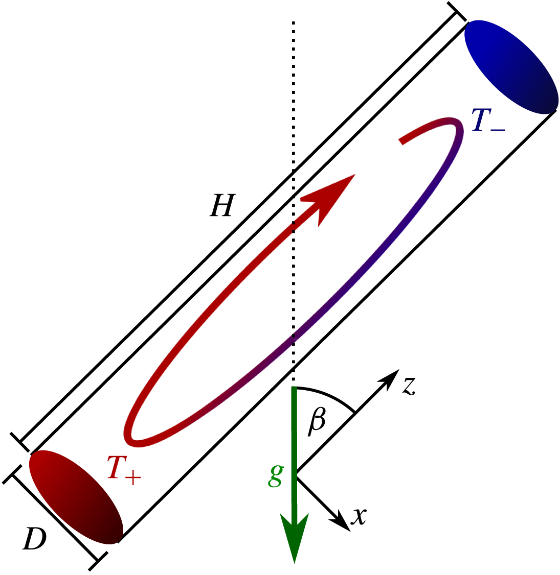
denotes the time- and volume-averaged heat transport parallel to the plates in the
 $x$
direction (see figure 1). For the two limiting cases of RBC (
 $\unicode[STIX]{x1D6FD}=0$
) and VC (
 $\unicode[STIX]{x1D6FD}=\unicode[STIX]{x03C0}/2$
) we get
 $$\begin{eqnarray}\displaystyle \langle \unicode[STIX]{x1D700}_{u}\rangle _{\unicode[STIX]{x1D6FD}=0}=\unicode[STIX]{x1D6FC}g\langle Tu_{z}\rangle & & \displaystyle\end{eqnarray}$$
and
 $$\begin{eqnarray}\displaystyle \langle \unicode[STIX]{x1D700}_{u}\rangle _{\unicode[STIX]{x1D6FD}=\unicode[STIX]{x03C0}/2}=-\unicode[STIX]{x1D6FC}g\langle Tu_{\Vert }\rangle , & & \displaystyle\end{eqnarray}$$
respectively. From (2.13) and the definition of the Nusselt number (2.4) we obtain
 $$\begin{eqnarray}\frac{H^{4}}{\unicode[STIX]{x1D708}^{3}}\frac{Pr^{2}}{Ra}\frac{\langle \unicode[STIX]{x1D700}_{u}\rangle }{Nu-1}=\cos \unicode[STIX]{x1D6FD}-\frac{\langle Tu_{\Vert }\rangle }{\langle Tu_{z}\rangle }\sin \unicode[STIX]{x1D6FD}.\end{eqnarray}$$
This equation shows how the ratio of
 $\langle \unicode[STIX]{x1D700}_{u}\rangle$
and the Nusselt number depends on the inclination angle. Note that
 $\langle Tu_{\Vert }\rangle /\langle Tu_{z}\rangle$
depends on the inclination angle as well.
Sketch of an inclined convection set-up. Here
 $D$
is the diameter,
 $H$
is the height of the cylinder,
 $\unicode[STIX]{x1D6FD}$
is the inclination angle,
 $T_{+}$
(
 $T_{-}$
) is the temperature of the hot (cold) plate and
 $g$
is the acceleration due to gravity.

2.3 Direct numerical simulations and mesh resolution
To investigate inclined thermal convection, three-dimensional DNS were performed in a cylindrical domain. The momentum and energy equations (2.1) and (2.2) are solved by the Goldfish code (Shishkina et al.
Reference Shishkina, Horn, Wagner and Ching2015; Shishkina & Horn Reference Shishkina and Horn2016; Shishkina & Wagner Reference Shishkina and Wagner2016; Kooij et al.
Reference Kooij, Botchev, Frederix, Geurts, Horn, Lohse, van der Poel, Shishkina, Stevens and Verzicco2018). The utilized mesh needs to resolve the smallest scales of the flow like the Batchelor and Kolmogorov scales (Shishkina et al.
Reference Shishkina, Stevens, Grossmann and Lohse2010). Since here we consider the case of
 $Pr\leqslant 1$
, the Kolmogorov scale
 $\unicode[STIX]{x1D702}=(\unicode[STIX]{x1D708}^{3}/\unicode[STIX]{x1D700}_{u})^{1/4}$
is the most demanding scale in our DNS. As a finite volume scheme is used in the simulations, the local characteristic mesh size is defined as
 $h=(r\unicode[STIX]{x1D6E5}_{r}\unicode[STIX]{x1D6E5}_{\unicode[STIX]{x1D719}}\unicode[STIX]{x1D6E5}_{z})^{1/3}$
, where
 $\unicode[STIX]{x1D6E5}_{r}$
,
 $\unicode[STIX]{x1D6E5}_{\unicode[STIX]{x1D719}}$
and
 $\unicode[STIX]{x1D6E5}_{z}$
are the local mesh spacings in the
 $r$
,
 $\unicode[STIX]{x1D719}$
and
 $z$
directions, respectively. For a good mesh resolution
 $h$
should be less than or at least similar to
 $\unicode[STIX]{x1D702}$
. This ratio
 $h/\unicode[STIX]{x1D702}$
is a local quantity, since a non-equidistant mesh is used and the kinetic energy dissipation rate varies locally as well. To get a single characteristic number to describe the mesh resolution, the maximum of the average in the
 $\unicode[STIX]{x1D719}$
direction is used:
 $$\begin{eqnarray}h_{\unicode[STIX]{x1D702}}=\max _{r,z}\langle h/\unicode[STIX]{x1D702}\rangle _{t,\unicode[STIX]{x1D719}}.\end{eqnarray}$$
Furthermore, deviations from the exact relations (2.12) and (2.13) can serve as reliable indicators for the accuracy of the numerical simulations. Therefore we also monitor the quantities
 $$\begin{eqnarray}{\mathcal{E}}_{u}\equiv \max _{\unicode[STIX]{x1D6FD}\in [0,\unicode[STIX]{x03C0}/2)}\left\{\frac{H^{4}}{\unicode[STIX]{x1D708}^{3}}\frac{Pr^{2}}{Ra}\frac{\langle \unicode[STIX]{x1D700}_{u}\rangle +\unicode[STIX]{x1D6FC}g\langle Tu_{\Vert }\rangle \sin \unicode[STIX]{x1D6FD}}{(Nu-1)\cos \unicode[STIX]{x1D6FD}}-1\right\}\end{eqnarray}$$
(for
 $\unicode[STIX]{x1D6FD}<\unicode[STIX]{x03C0}/2$
only, since the limit
 $\unicode[STIX]{x1D6FD}\rightarrow \unicode[STIX]{x03C0}/2$
is difficult to obtain numerically) and
 $$\begin{eqnarray}{\mathcal{E}}_{\unicode[STIX]{x1D703}}\equiv \max _{\unicode[STIX]{x1D6FD}\in [0,\unicode[STIX]{x03C0}/2]}\left\{\frac{H^{2}}{\unicode[STIX]{x1D705}\unicode[STIX]{x1D6E5}^{2}}\frac{\langle \unicode[STIX]{x1D700}_{\unicode[STIX]{x1D703}}\rangle }{Nu}-1\right\}.\end{eqnarray}$$
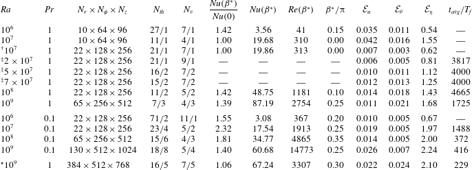
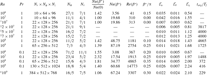
In table 1 these values as well as the number of mesh points are listed for all performed simulations. Additionally, for
 $Ra=10^{7}$
,
 $Pr=1$
,
 $\unicode[STIX]{x1D6FD}/\unicode[STIX]{x03C0}=0$
and
 $\unicode[STIX]{x1D6E4}=1/5$
a simulation was run also on a finer mesh, similar to the one for
 $Ra=10^{8}$
. It showed good agreement with the lower resolved mesh: averaged quantities such as the Nusselt number and Reynolds number deviate only approximately 1 %.
Overview of the conducted simulations: the Rayleigh number
 $Ra$
, Prandtl number
 $Pr$
, number of computational mesh points
 $N_{i}$
in all three directions (
 $r,\unicode[STIX]{x1D719},z$
), number of points inside the thermal BL
 $N_{th}$
and viscous BL
 $N_{v}$
compared to required number of points inside the BL according to Shishkina et al. (Reference Shishkina, Stevens, Grossmann and Lohse2010) (note that here, for each case, we calculate the parameter
 $a$
in equation (14) of Shishkina et al. (Reference Shishkina, Stevens, Grossmann and Lohse2010) from the Reynolds number
 $Re_{w}$
and viscous BL thickness, since for the aspect ratio
 $\unicode[STIX]{x1D6E4}=1/5$
it is approximately 2.5 times smaller than originally estimated), maximum relative increase of the Nusselt number
 $Nu$
(2.4) at the optimal inclination angle
 $\unicode[STIX]{x1D6FD}^{\ast }$
, Nusselt number
 $Nu$
and Reynolds number
 $Re$
(2.5) at the optimal inclination angle, maximal (over all inclinations angles) deviation of the exact dissipation relations (2.18) and (2.19), characteristic mesh resolution
 ${\mathcal{E}}_{\unicode[STIX]{x1D702}}=\max _{\unicode[STIX]{x1D6FD}}h_{\unicode[STIX]{x1D702}}$
(2.17) and the shortest averaging time
 $t_{avg}$
(for unsteady flows), normalized with
 $T_{f}\equiv \sqrt{R/(\unicode[STIX]{x1D6FC}g\unicode[STIX]{x1D6E5})}$
(no averaging time is given if the flow is steady for all
 $\unicode[STIX]{x1D6FD}$
). Note that for all presented cases 11 different inclination angles
 $\unicode[STIX]{x1D6FD}$
,
 $0\leqslant \unicode[STIX]{x1D6FD}\leqslant \unicode[STIX]{x03C0}/2$
, were considered.
 $^{\star }$
The aspect ratio is
 $\unicode[STIX]{x1D6E4}=1/5$
, except for the last row, marked by
 $^{\star }$
, which has the aspect ratio
 $\unicode[STIX]{x1D6E4}=1$
.
 $^{\dagger }$
Only five different inclination angles used.
 $^{\ddagger }$
Only RBC (
 $\unicode[STIX]{x1D6FD}/\unicode[STIX]{x03C0}=0$
).
3 Results
3.1 The effect of inclination
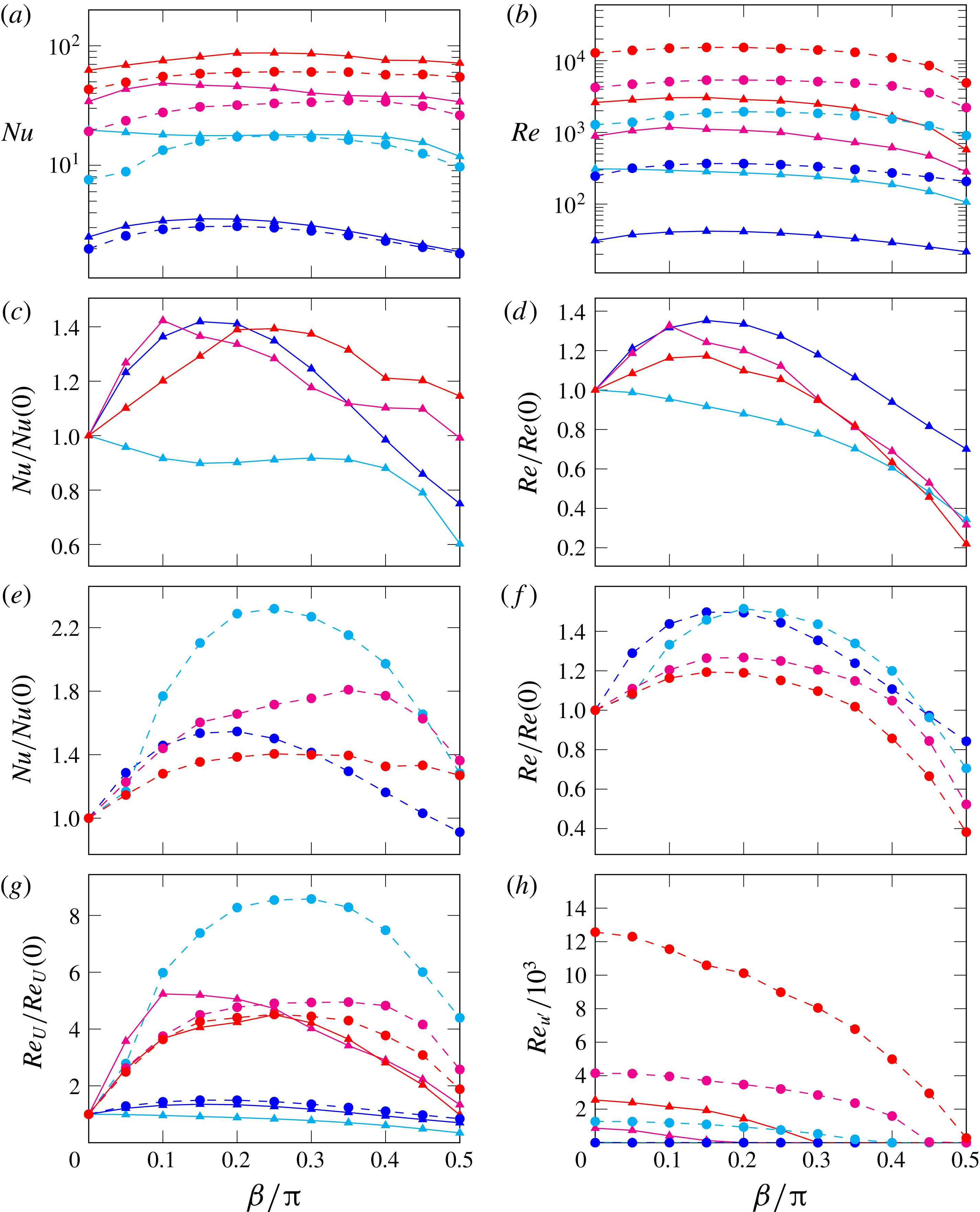
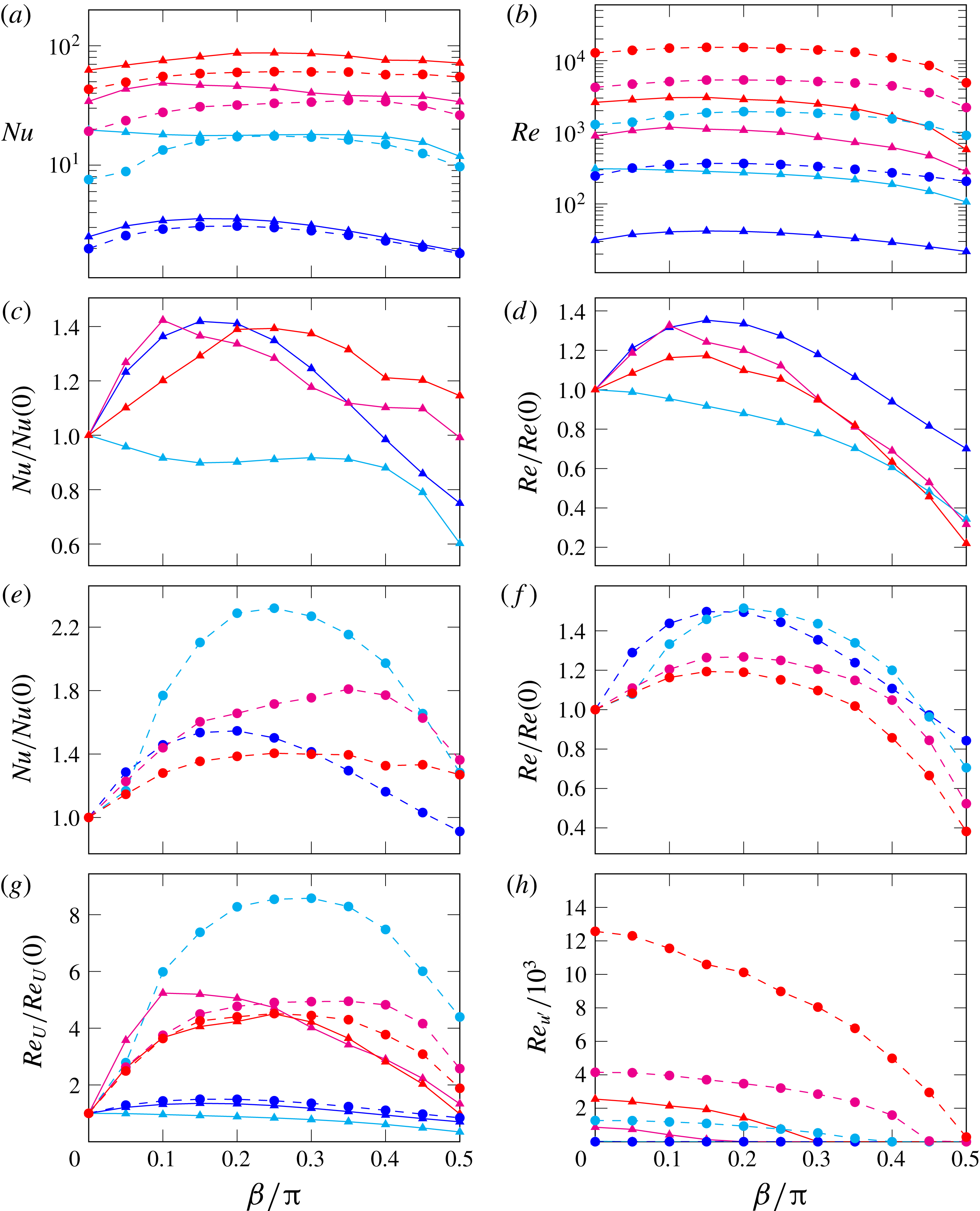
We consider the global transport quantities in the case of inclined convection. Inclination of the cell, in the investigated parameter range, usually leads to an increase in the global heat transport until a certain optimal inclination angle
 $\unicode[STIX]{x1D6FD}^{\ast }$
where the heat transport is maximal. Further inclination leads to a decrease of the global heat transport (see figure 2
a,c,e). For the Reynolds number,
 $Re$
, based on the kinetic energy (2.5), the behaviour with inclination is similar to that for the heat transport. However, the maximum of the Reynolds number, based on kinetic energy, is usually observed for angles smaller than or equal to
 $\unicode[STIX]{x1D6FD}^{\ast }$
and the relative decrease of
 $Re$
is much stronger near the VC case (see figure 2
b,d,f). Also, the relative increase of the Reynolds number is usually less than the relative increase of the Nusselt number (cf. figure 2
c,e with 2
d,f). The only exception to the above observations is the case of
 $Pr=1$
and
 $Ra=10^{7}$
, where inclination always leads to a decrease of the heat and momentum transport. The reason for this will be discussed further below.
The absolute and normalized (with respect to RBC) Nusselt and Reynolds numbers plotted against the inclination angle
 $\unicode[STIX]{x1D6FD}$
for
 $Pr=1$
(solid lines) and
 $Pr=0.1$
(dashed lines). Rayleigh numbers are
 $10^{6}$
(blue),
 $10^{7}$
(cyan),
 $10^{8}$
(magenta) and
 $10^{9}$
(red). (a) Absolute Nusselt number. (b) Absolute Reynolds number, based on kinetic energy. (c) Normalized Nusselt number for
 $Pr=1$
. (d) Normalized Reynolds number for
 $Pr=1$
.(e) Normalized Nusselt number for
 $Pr=0.1$
. (f) Normalized Reynolds number for
 $Pr=0.1$
. (g) Normalized large-scale Reynolds number. (h) Absolute small-scale Reynolds number.
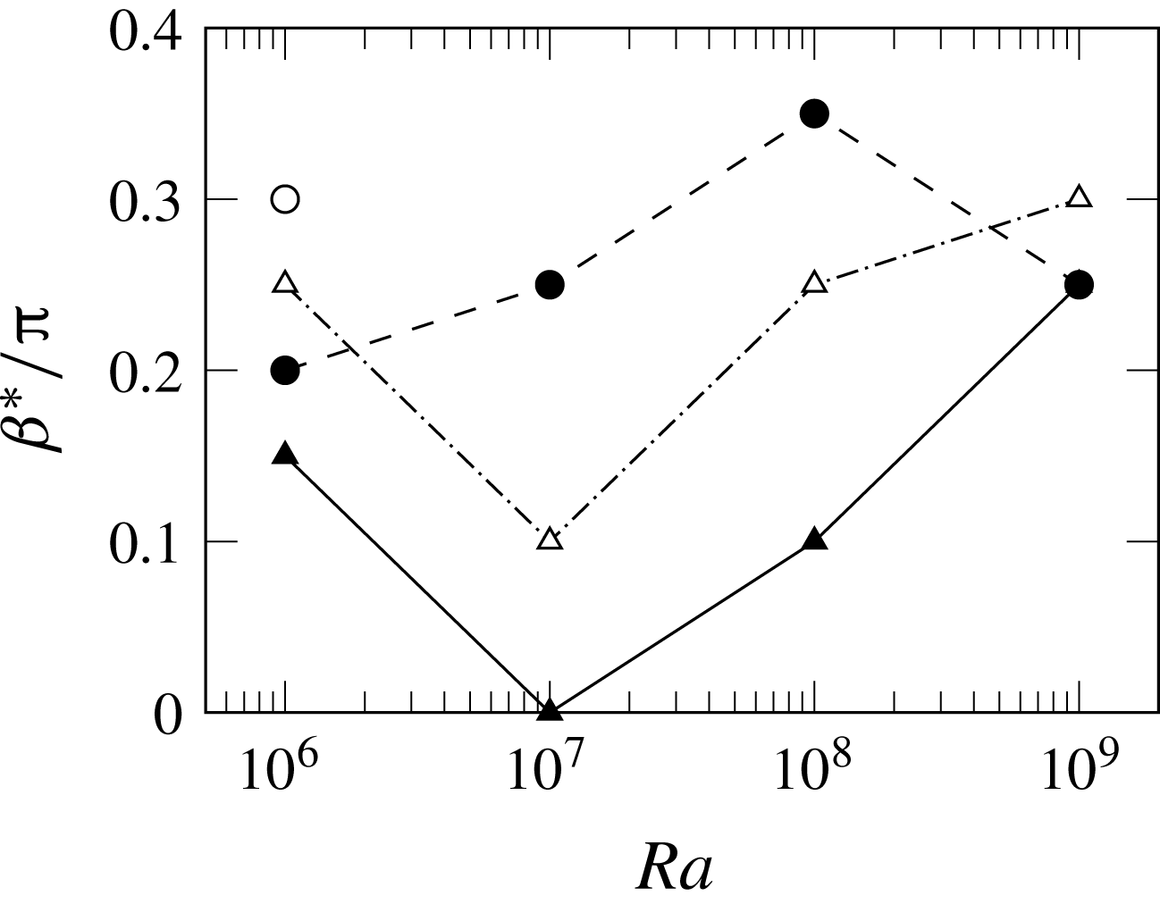
Inclination angle
 $\unicode[STIX]{x1D6FD}^{\ast }$
for the optimal heat transport, as a function of
 $Ra$
, for
 $Pr=1$
(triangles) and
 $Pr=0.1$
(circles), for the aspect ratios
 $\unicode[STIX]{x1D6E4}=1/5$
(filled symbols) and
 $\unicode[STIX]{x1D6E4}=1$
(open symbols). The data for
 $\unicode[STIX]{x1D6E4}=1$
,
 $Ra<10^{9}$
are adapted from Shishkina & Horn (Reference Shishkina and Horn2016).

Vertical cross-sections through the instantaneous flow fields for
 $Pr=1$
and (a)
 $Ra=10^{6}$
, (b)
 $Ra=10^{7}$
, (c)
 $Ra=10^{8}$
and (d)
 $Ra=10^{9}$
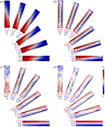
. The colour scale is from hot (red) to cold (blue). The numbers are (from top) the Nusselt number (red), Reynolds number (blue) and inclination angle
 $\unicode[STIX]{x1D6FD}/\unicode[STIX]{x03C0}$
(black). The thickness of the black streamlines reflects the normalized velocity magnitude.

Vertical cross-sections through the instantaneous flow fields for
 $Pr=0.1$
and (a)
 $Ra=10^{6}$
, (b)
 $Ra=10^{7}$
, (c)
 $Ra=10^{8}$
and (d)
 $Ra=10^{9}$
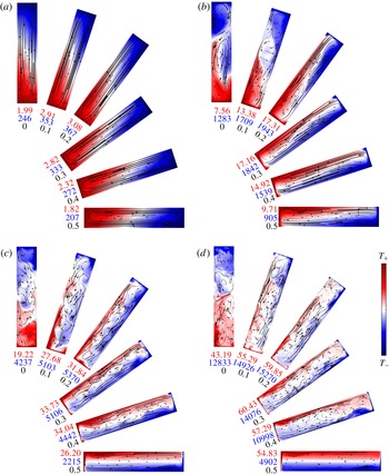
. The numbers are (from top) the Nusselt number (red), Reynolds number (blue) and inclination angle
 $\unicode[STIX]{x1D6FD}/\unicode[STIX]{x03C0}$
(black). Colour scale and streamlines as in figure 4.

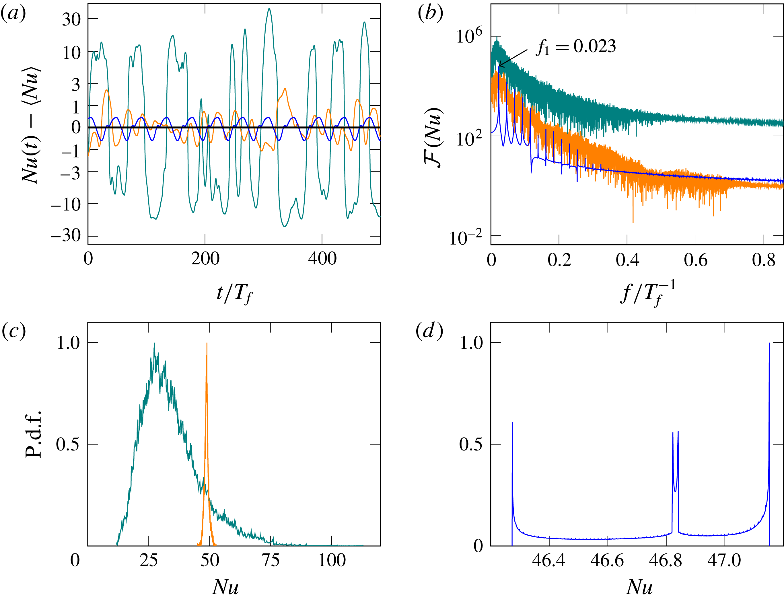
The temporal behaviour of the Nusselt number for
 $Ra=10^{8}$
,
 $Pr=1$
,
 $\unicode[STIX]{x1D6E4}=1/5$
and
 $\unicode[STIX]{x1D6FD}/\unicode[STIX]{x03C0}=0$
(green),
 $\unicode[STIX]{x1D6FD}/\unicode[STIX]{x03C0}=0.1$
(orange) and
 $\unicode[STIX]{x1D6FD}/\unicode[STIX]{x03C0}=0.15$
(blue). The time scale is based on
 $T_{f}=\sqrt{R/(\unicode[STIX]{x1D6FC}g\unicode[STIX]{x1D6E5})}$
. (a) Deviations of the Nusselt number from its mean value (note that the positive and negative scale is logarithmic) versus time. (b) Amplitude of the Fourier spectrum
 ${\mathcal{F}}$
of the Nusselt number. (c,d) Probability density functions (p.d.f.) of the Nusselt number normalized by the respective maximum. Here the instantaneous Nusselt number
 $Nu(t)$
is determined by averaging over the entire volume.

The inclination angle
 $\unicode[STIX]{x1D6FD}^{\ast }$
for the optimal heat transport is plotted against the Rayleigh number in figure 3. The figure shows that
 $\unicode[STIX]{x1D6FD}^{\ast }$
depends non-monotonically on
 $Ra$
. However, one can see that, at a lower Prandtl number and/or larger aspect ratio, the optimal heat transport is reached at a larger inclination angle.
A closer look at the instantaneous flow fields (see figure 4 for
 $Pr=1$
and figure 5 for
 $Pr=0.1$
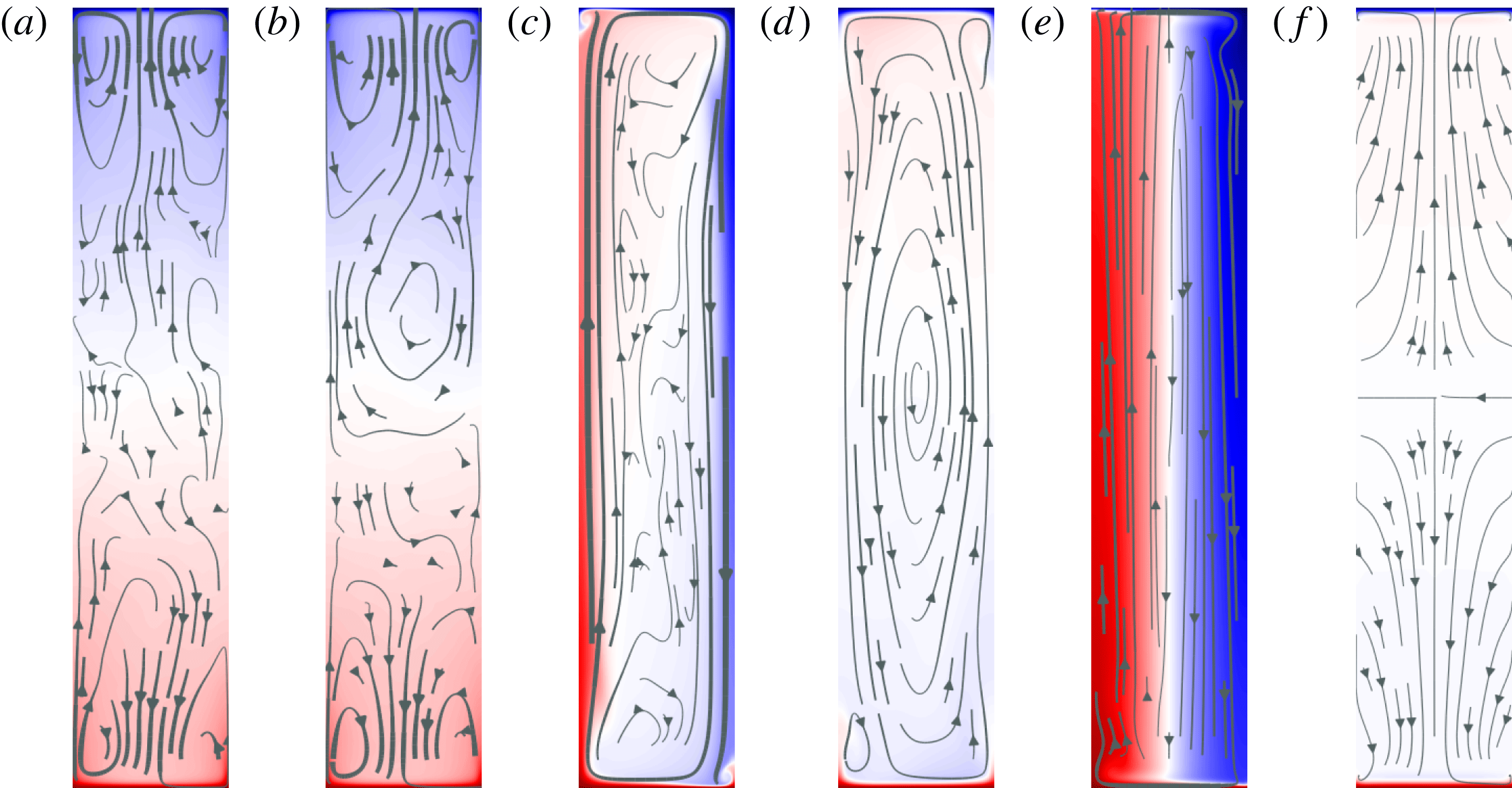
) reveals some expected and also some new features, which can be associated with the inclination. Inclining the cylinder forces the direction of the LSC to be fixed, which results in a very structured flow. This is illustrated by those flow fields in figures 4 and 5, where the streamlines align nicely in the case of inclined convection.
At the lowest Rayleigh number,
 $Ra=10^{6}$
, the spatial temperature distribution is similar to that of the conductive case and there are no single plumes visible for either of the investigated Prandtl numbers. These flow states are steady solutions of the governing equations (2.1) and (2.2) because the Reynolds number based on the velocity fluctuations,
 $Re_{u^{\prime }}$
, vanishes. Additionally, the streamlines are aligned and show a flow field with a smooth laminar-like LSC (see figures 4
a and 5
a).
While increasing the Rayleigh number and thus the thermal driving (
 $Ra=10^{7}$
,
 $Pr=1$
), we still observe a laminar-like flow with an LSC but the spatial temperature distribution looks completely different now (figure 4
b). The temperature at the rising/falling side of the LSC is close to the temperature of the respective BL. This picture is reminiscent of hot/cold channels or plume columns which span the whole cylinder and is observed for all inclination angles. Nevertheless, in this case there are no distinguishable plumes apart from the rising/falling ones and the flow is also laminar-like. As we will see, these plume columns appear to play an important role in the increase of the heat transport in inclined convection (cf. § 3.2).
For
 $Ra=10^{7}$
and
 $Pr=1$
, the RBC flow provides the optimal heat transport. This can be explained by the fact that the plume columns are already present in the flow configuration without inclination (
 $\unicode[STIX]{x1D6FD}/\unicode[STIX]{x03C0}=0$
) (see figure 4
b), while the strength of the LSC decreases with increasing inclination (cf. figure 2
c,g).
A further increase of the Rayleigh number to
 $Ra=10^{8}$
leads to the development of quite a vigorous flow in RBC (see figure 4
c,
 $\unicode[STIX]{x1D6FD}=0$
) and in this case the rising and falling plumes appear chaotically, leading to a complicated flow structure (see supplementary movie 1 available at https://doi.org/10.1017/jfm.2018.477). Also, the small-scale Reynolds number (
 $Re_{u^{\prime }}=865$
) is no longer vanishing, which means that there are significant fluctuations in the velocity field. Inclining the cell leads to a decrease in the small-scale Reynolds number (figure 2
h, solid magenta line), and for an inclination angle of
 $\unicode[STIX]{x1D6FD}\approx 0.2\unicode[STIX]{x03C0}$
, the flow becomes steady. The emergence of the plume columns is observed at
 $\unicode[STIX]{x1D6FD}=0.1\unicode[STIX]{x03C0}$
, where also the maximal Nusselt number is obtained (cf. figure 4
b,c). Furthermore, the large-scale Reynolds number reaches its maximum there too, while the small-scale Reynolds number decreases by approximately 50 % compared to that in RBC.
Except for the case of highest Rayleigh number,
 $Ra=10^{9}$
, and lowest Prandtl number,
 $Pr=0.1$
, we always observe a transition to a steady flow field when the inclination angle is increased. Hence, we will discuss this transition to steady flow using this parameter set of
 $Ra=10^{8}$
and
 $Pr=1$
as an example, since it demonstrates all kinds of behaviour, from a turbulent flow in RBC to the formation of plume columns, as well as an oscillatory state and finally, for a sufficiently large inclination angle, a steady flow. Therefore, we pick the five most interesting inclination angles, namely
 $\unicode[STIX]{x1D6FD}/\unicode[STIX]{x03C0}=0$
(RBC),
 $\unicode[STIX]{x1D6FD}^{\ast }/\unicode[STIX]{x03C0}=0.1$
(optimal heat transport),
 $\unicode[STIX]{x1D6FD}/\unicode[STIX]{x03C0}=0.15$
(oscillatory state),
 $\unicode[STIX]{x1D6FD}/\unicode[STIX]{x03C0}\approx 0.2$
(steady flow) and
 $\unicode[STIX]{x1D6FD}=\unicode[STIX]{x03C0}/2$
(VC) to discuss the behaviour. The time evolution of the Nusselt number is displayed in figure 6(a), and for a better understanding we also provide the amplitude of the Fourier spectrum (figure 6
b) and the probability density function (p.d.f.) of the Nusselt number (figure 6
c,d).
In RBC we observe strong fluctuations of the Nusselt number, where the standard deviation is approximately 35 % of the mean value and the p.d.f. shows a wide tail at higher Nusselt numbers. In the case of optimal heat transport (
 $\unicode[STIX]{x1D6FD}=0.1\unicode[STIX]{x03C0}$
), the probability density function of the Nusselt number is narrow, almost symmetric, and the standard deviation is only approximately 1.8 % of the mean value. The width of the p.d.f. of the Nusselt number is decreasing with inclination, which is due to the strong stratification of the flow. The third case, as already mentioned, is special, because we observe an oscillatory state that leads to a periodic variation of the Nusselt number. The main frequency is
 $f_{1}=0.023T_{f}^{-1}$
and the Fourier spectrum (figure 6
b) also shows multiples of this main frequency. Apparently this frequency is also characteristic (strongest) for the less inclined cases, which show a continuous spectrum. Below, the oscillating case will be further discussed. At
 $\unicode[STIX]{x1D6FD}/\unicode[STIX]{x03C0}\approx 0.2$
, the flow becomes steady and the Nusselt number no longer changes in time, so it is of no interest to look at the p.d.f. or spectrum for any larger inclination angles. In VC we observe a temperature distribution which is strongly stratified with respect to the direction of gravity. For large
 $Ra$
and
 $Pr=0.1$
, the Nusselt numbers in VC are larger than those in RBC (cf. figure 2
e).
Supplementary movie 2 shows the temperature isosurfaces of the oscillating flow field (
 $\unicode[STIX]{x1D6FD}/\unicode[STIX]{x03C0}=0.15$
). There is a torsional oscillation visible in the flow, which is asymmetric in azimuthal direction. Oscillating states were also observed for RBC in an aspect-ratio-one cell between the onset of convection and fully turbulent flow, by Verzicco & Camussi (Reference Verzicco and Camussi1997). This suggests that the route to turbulence in inclined convection is similar to RBC.
The qualitative picture of the flow structure, i.e. the emergence of plume columns, at the optimal inclination angle
 $\unicode[STIX]{x1D6FD}^{\ast }$
(with respect to the Nusselt number) appears to be similar for both investigated Prandtl numbers and
 $Ra\geqslant 10^{7}$
. This means that the maximal heat transport is reached as soon as the plume columns are fully developed, i.e. they span the whole cylinder, and the large-scale Reynolds number is also very close to its maximal value. Thus, our simulations evince similar behaviour of the small- and large-scale Reynolds number as observed in the LES by Teimurazov & Frick (Reference Teimurazov and Frick2017). They claimed that these observations are an indicator that the LSC is playing an important role in the heat transport in inclined convection.
As expected, for a lower Prandtl number (
 $Pr=0.1$
) turbulent flows are obtained already at lower Rayleigh numbers and they remain turbulent until larger inclination angles. This is underlined quantitatively by the small-scale Reynolds numbers, which are plotted in figure 2(h). One can see from these data that the transition from a turbulent to a steady flow happens at larger inclination angles for lower Prandtl numbers or higher Rayleigh numbers.
Although the Prandtl number in the experiments by Frick et al. (Reference Frick, Khalilov, Kolesnichenko, Mamykin, Pakholkov, Pavlinov and Rogozhkin2015) and LES by Teimurazov & Frick (Reference Teimurazov and Frick2017) is significantly lower than
 $Pr=0.1$
, there are certain similarities between our and their results. We obtained a similar relative increase of the heat transport (
 $Nu(\unicode[STIX]{x1D6FD}^{\ast })/Nu(0)$
). The studies showed also that, for otherwise similar set of parameters, a higher Nusselt number is obtained in VC rather than in RBC. In both the LES and our DNS, similar temperature profiles were obtained that demonstrated a non-vanishing gradient of the mean temperature in the bulk in RBC and vanishing gradient in inclined and vertical convection.
The highest relative increase in heat transport is observed for Rayleigh number
 $Ra=10^{7}$
and Prandtl number
 $Pr=0.1$
. We see a vigorous flow,
 $Re_{u^{\prime }}=756$
, and system-sized plume column formation that finally leads to an approximately 2.3 times stronger heat transport in the inclined case (
 $\unicode[STIX]{x1D6FD}^{\ast }\approx 0.25\unicode[STIX]{x03C0}$
) compared to that in RBC.
3.2 Plume columns and the flow structure of enhanced heat transfer
Since the plume columns appear to increase the heat transport as soon as they span the whole cylinder and, therefore, impinge on the opposite boundary layer, one might also compare the situation in inclined convection with that of impinging jets on a surface. When a jet impinges on a hot surface, the heat transport depends on many parameters, such as the Reynolds number, Prandtl number, ratio of plate distance to nozzle diameter, and radial distance from the stagnation point (Jambunathan et al.
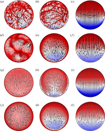
Reference Jambunathan, Lai, Moss and Button1992). It is known that the heat transport is generally larger in an impinging jet rather than in a parallel flow, but the heat transport decreases with the distance from the stagnation point of the jet. This was shown by various experiments such as those by Huang & El-Genk (Reference Huang and El-Genk1994). Under the assumption that the fully developed plume columns, spanning the whole cylinder, act like a jet impinging on a surface, it is reasonable to assume that this might cause the strongly increased heat transport. Additionally, such impinging zones are clearly seen in figure 7(h,k). From these panels it is apparent that the ratio of the impinging area to the plate area is much smaller in aspect ratio
 $\unicode[STIX]{x1D6E4}=1$
compared to
 $\unicode[STIX]{x1D6E4}=1/5$
and the heat transport behaves similarly, i.e. it is higher inside the slender cylinder. For a thorough analysis of the aspect ratios, see § 3.4.
Our slender geometry also shows some similarities of heat transport through an inclined vertical channel. Riedinger et al. (Reference Riedinger, Tisserand, Seychelles, Castaing and Chillà2013) carried out such experiments with a square channel of aspect ratio
 $1/4$
, where the ends of the channel are connected to a hot/cold reservoir of water. They found similar behaviour in the inclined channel, like stratification due to gravity, and an apparently higher scaling exponent in the transition region to the turbulent regime (as discussed below in § 3.5). Furthermore, they also observed two non-mixing symmetrical jets with inclination angle
 $\unicode[STIX]{x1D6FD}/\unicode[STIX]{x03C0}>0$
.
In general, stratification of the temperature field, which is induced by the cell inclination, supports the formation of the plume columns. On the other hand, high Rayleigh numbers enhance the turbulent mixing and thus break apart the plume columns. All this leads to the conclusion that, for larger
 $Ra$
, the optimal heat transfer is to be expected at larger values of
 $\unicode[STIX]{x1D6FD}/\unicode[STIX]{x03C0}$
. A careful interpretation of figure 3 supports this trend. Here, one has to keep in mind that the plume columns exist only for
 $Ra\geqslant 10^{7}$
.
Cross-sections parallel to the heated plate at the edge of the thermal BL (
 $z=\unicode[STIX]{x1D6FF}_{T}=H/(2Nu)$
) for
 $Ra=10^{9}$
and
 $Pr=1$
of (a–f) the instantaneous and (g–l) the time-averaged temperature and velocity fields (colour scale and streamlines as in figure 4). The aspect ratios are (a–c, g–i)
 $\unicode[STIX]{x1D6E4}=1$
and (d–f, j–l)
 $\unicode[STIX]{x1D6E4}=1/5$
. All cross-sections are taken for three different inclination angles
 $\unicode[STIX]{x1D6FD}/\unicode[STIX]{x03C0}=0$
(first column),
 $\unicode[STIX]{x1D6FD}/\unicode[STIX]{x03C0}=0.25$
(second column) and
 $\unicode[STIX]{x1D6FD}/\unicode[STIX]{x03C0}=0.5$
(third column). The inner circles in (a–c) show the area of the cross-section in the case of
 $\unicode[STIX]{x1D6E4}=1/5$
for the same height as in (d–f), respectively.

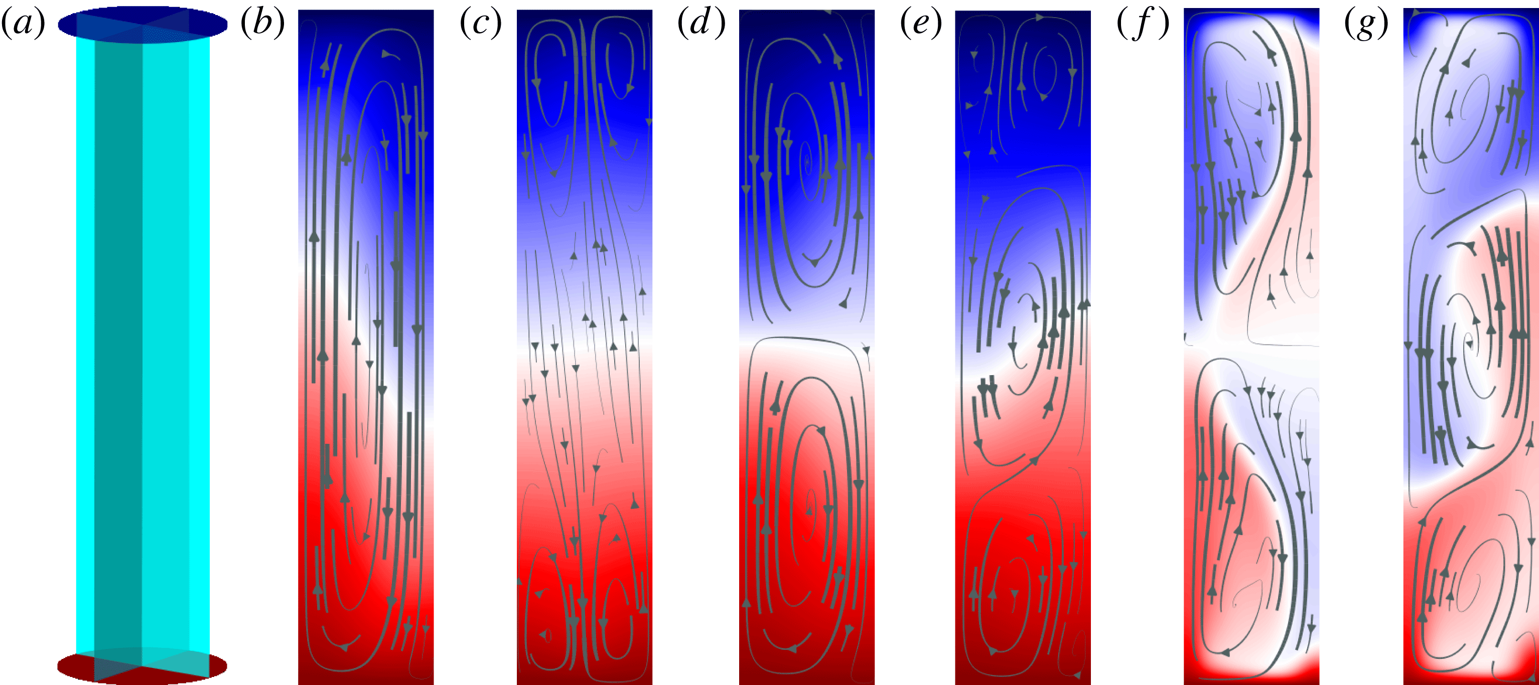
Vertical cross-sections sketched in (a) through the instantaneous flow fields of (b,c) the single-roll state for
 $Ra=10^{6}$
and
 $Pr=0.1$
, (d,e) the double-roll state for
 $Ra=10^{6}$
and
 $Pr=0.1$
, and (f,g) the double-roll state for
 $Ra=10^{7}$
and
 $Pr=1$
. Vertical cross-sections through (b,d,f) the plane of the rolls and (c,e,g) the plane perpendicular to it. Colour scale and streamlines as in figure 4.

It is necessary to further discuss the physical processes that support the formation of plume columns, since the reported findings indicate the importance of the emerging plume columns to the increase in heat transport. Therefore, let us consider a hot thermal plume or some small patch of hot fluid that has just detached from the thermal BL and what will happen to it afterwards. There are two relevant time scales: the time that the plume needs to travel to the opposite BL, and the thermal diffusion time, during which the plume loses its thermal energy to the surrounding fluid. First, the thermal plume is collected by the LSC and therefore accelerates to the velocity of the LSC,
 $U=\sqrt{\langle \langle \boldsymbol{u}\rangle _{t}^{2}\rangle _{V}}$
(as used in (2.9)), which gives the travelling time scale,
 $\unicode[STIX]{x1D70F}_{u}=H/U$
. The relevant length scale for the travelling time is the height of the cylinder
 $H$
, whereas we set the radius
 $R$
as the relevant length scale for the thermal diffusion time,
 $\unicode[STIX]{x1D70F}_{\unicode[STIX]{x1D705}}=R^{2}/\unicode[STIX]{x1D705}$
, since this is the approximate lateral extent the plume can gain before it will interact with the cold plume channel. The lateral viscous diffusion time,
 $R^{2}/\unicode[STIX]{x1D708}$
, is longer and hence not important in these considerations for
 $Pr\leqslant 1$
. Plume columns can be formed if the travelling time is less than or approximately the same as the thermal diffusion time,
 $H/U\lessapprox R^{2}/\unicode[STIX]{x1D705}$
. From this we can estimate a threshold for our large-scale Reynolds number that is necessary to produce plume columns:
 $4\unicode[STIX]{x1D6E4}^{2}Re_{U}Pr\gtrapprox 1$
. As already discussed for
 $Ra=10^{6}$
and both Prandtl numbers, we have a profile that is close to the conductive temperature distribution (no plume columns) and indeed we find
 $4\unicode[STIX]{x1D6E4}^{2}Re_{U}Pr<1$
. For
 $Ra=10^{7}$
and
 $Pr=1$
we observe plume columns and
 $4\unicode[STIX]{x1D6E4}^{2}Re_{U}Pr\approx 3$
. A further condition for the plume columns to exist is that the velocity fluctuations must not prevail over the mean flow.
3.3 Single-roll and double-roll states in Rayleigh–Bénard convection
For the RBC case of this parameter set, we find two possible states: a single-roll state and a double-roll state (figure 8). The single-roll state is used as the reference case for the relative change of the Nusselt number and Reynolds number, because in inclined convection the single-roll state dominates. As known, for example, from experiments by Xi & Xia (Reference Xi and Xia2008) and Weiss & Ahlers (Reference Weiss and Ahlers2013), the heat flux in the double-roll state is smaller compared to that in a single-roll state. Our simulations confirm this fact, and we find a strong reduction, i.e. the heat transport in the double-roll state is only approximately 80 % of the heat transport in the single-roll state for
 $Ra=10^{6}$
and
 $Pr=0.1$
(figure 8
b–e). There is one further case where we observe a single-roll state and a double-roll state, which is
 $Ra=10^{7}$
and
 $Pr=1$
(figures 4
b and 8
f,g).
Both states are steady (vanishing velocity fluctuations) but their occurrence depends on the initial flow fields of the simulation. This means that, unlike the experiment by Weiss & Ahlers (Reference Weiss and Ahlers2013), transitions between these states are not to be expected.
For a slightly higher Rayleigh number,
 $Ra=2\times 10^{7}$
, we tried to find both states as well, but initiating the simulations from the single-roll state leads to the double-roll state. This suggests that the double-roll state might be the preferred state; however, finding the probability of each state is computationally too expensive. At the Rayleigh number
 $Ra=5\times 10^{7}$
and higher, there is no long-term LSC present any more. This is caused by the small aspect ratio, as we will discuss in § 3.4.
3.4 The effect of confinement
To investigate the influence of the aspect ratio on the transport quantities, as well as on the flow structure, simulation data for
 $Ra=10^{9}$
,
 $Pr=1$
and 11 different inclination angles
 $\unicode[STIX]{x1D6FD}$
are compared for the aspect ratios
 $\unicode[STIX]{x1D6E4}=1$
and
 $\unicode[STIX]{x1D6E4}=1/5$
. Thereby, a special focus lies on the cases of RBC (
 $\unicode[STIX]{x1D6FD}/\unicode[STIX]{x03C0}=0$
), the optimal inclination angle (
 $\unicode[STIX]{x1D6FD}=\unicode[STIX]{x1D6FD}^{\ast }$
) and VC (
 $\unicode[STIX]{x1D6FD}/\unicode[STIX]{x03C0}=0.5$
).
In RBC both aspect ratios have similar values of the Nusselt numbers, where
 $Nu\;(\unicode[STIX]{x1D6E4}=1)$
is less than 2 % larger than
 $Nu\;(\unicode[STIX]{x1D6E4}=1/5)$
. Although the heat transport shows qualitatively similar behaviour with inclination in both cases, i.e. the heat transport increases with inclination, reaches a maximum at a certain inclination angle (in this case
 $\unicode[STIX]{x1D6FD}^{\ast }\approx \unicode[STIX]{x03C0}/4$
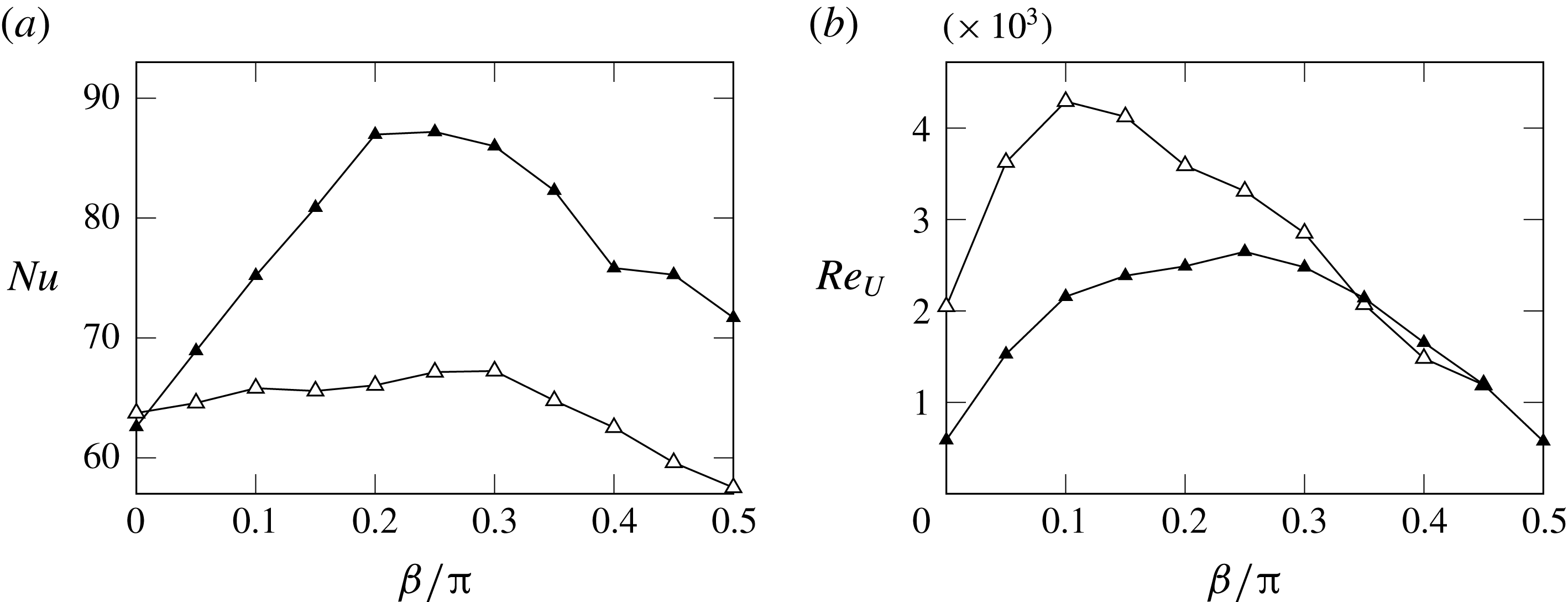
for both aspect ratios) and then decreases again, there are some important differences. The first and most apparent difference is the higher relative increase in the heat transport for the slender cylinder, which is approximately 40 % compared to only 6 % increase for the cylinder with aspect ratio one (figure 9
a). Furthermore, the small-aspect-ratio cylinder shows a larger heat transport for VC compared to RBC, but for the aspect-ratio-one cylinder VC has a lower heat transport compared to the respective RBC.
The Nusselt number and the different Reynolds numbers for
 $Ra=10^{9}$
and the aspect ratio
 $\unicode[STIX]{x1D6E4}=1$
(open triangles) and
 $\unicode[STIX]{x1D6E4}=1/5$
(filled triangles) plotted against the inclination angle
 $\unicode[STIX]{x1D6FD}$
. (a) Absolute Nusselt number. (b) Absolute large-scale Reynolds number
 $Re_{U}$
.

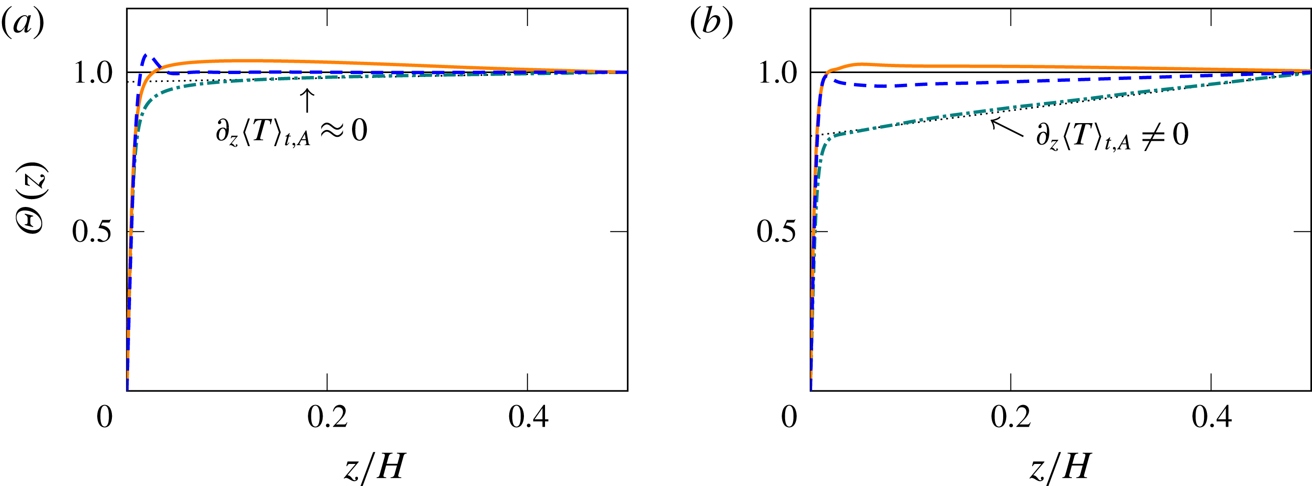
The normalized mean temperature profiles,
 $\unicode[STIX]{x1D6E9}(z)=2(T_{+}-\langle T\rangle _{t,A})/\unicode[STIX]{x1D6E5}$
, for
 $Ra=10^{9}$
,
 $Pr=1$
and three different inclination angles
 $\unicode[STIX]{x1D6FD}/\unicode[STIX]{x03C0}=0$
(green dash-dotted),
 $\unicode[STIX]{x1D6FD}/\unicode[STIX]{x03C0}=0.25$
(orange solid) and
 $\unicode[STIX]{x1D6FD}/\unicode[STIX]{x03C0}=0.5$
(blue dashed). The aspect ratios are (a)
 $\unicode[STIX]{x1D6E4}=1$
and (b)
 $\unicode[STIX]{x1D6E4}=1/5$
.

In contrast to the heat transport, the Reynolds number, based on the kinetic energy, is higher for all inclination angles in aspect ratio
 $\unicode[STIX]{x1D6E4}=1$
, whereas the relative increase with inclination is higher for the slender cylinder. This is due to the stabilizing effect of the slender geometry on the flow. A look at the large-scale Reynolds numbers
 $Re_{U}$
(figure 9
b) reveals that, in aspect ratio
 $\unicode[STIX]{x1D6E4}=1$
, the maximum is reached already at
 $\unicode[STIX]{x1D6FD}=0.1\unicode[STIX]{x03C0}$
, which is at a smaller inclination angle than the optimal one (
 $\unicode[STIX]{x1D6FD}^{\ast }=\unicode[STIX]{x03C0}/4$
). Above we discussed that for slender cylinders the points of the maxima of
 $Re_{U}$
and of the Nusselt number coincide, pointing out that the strength of the LSC is important for the increase in the heat transport (Teimurazov & Frick Reference Teimurazov and Frick2017). Also from the same figure we can see that, in aspect ratio one, there is a dominant LSC in RBC.
In figure 10 we compare the normalized temperature profiles, averaged in time and over cross-sections at distance
 $z$
from the heated plate, of the two aspect ratios, for the three cases: RBC, the optimal inclination angle and VC. The temperature is normalized in such a way that it is equal to zero at the heated plate and to one in the core part of the domain. The usual expectation of the temperature profile in RBC is that the temperature rises within the thermal BL close to the mean value, then in the bulk region it takes the mean value, hence the temperature gradient is approximately zero in the bulk. In the aspect-ratio-one case, we observe this expected behaviour, but in the slender cylinder, the temperature rises only to approximately
 $3/4$
of the bulk temperature within the thermal BL. This is accompanied by a non-zero temperature gradient inside the bulk region (see figure 10
b). At an inclination angle of
 $\unicode[STIX]{x1D6FD}=\unicode[STIX]{x03C0}/4$
, both aspect ratios show a slight inversion of the bulk temperature gradient, i.e. the sign of the temperature gradient changes compared to the gradient of the conductive profile. This kind of behaviour was previously observed by Scheel & Schumacher (Reference Scheel and Schumacher2016) for a very low Prandtl number,
 $Pr=0.005$
, in RBC inside an aspect-ratio-one cylinder. For vertical convection there is a slightly colder/warmer region above the hot/cold thermal BL. These regions show up as local extrema in the temperature profile and can also be seen in the vertical slices of the time-averaged fields (figures 11
c,f and 12
e,f). In the aspect ratio
 $\unicode[STIX]{x1D6E4}=1$
case, the region of the local extremum shows an inversion, which means that the layer of hot fluid above the BL has a temperature larger than the average temperature inside the bulk.
Thermal plumes are an important feature of turbulent thermal convection and, as mentioned above, the formation of plume columns apparently facilitates an increase of the heat transport. Further visualization of the flow field reveals how thermal plumes are influenced by inclination and the aspect ratio. Slices taken at the edge of the thermal BL,
 $z=\unicode[STIX]{x1D6FF}_{\unicode[STIX]{x1D703}}$
, of the instantaneous temperature and velocity fields are shown for both aspect ratios in figure 7(a–f). There is a visual aid (black circle) given to show the diameter of the small-aspect-ratio cylinder scaled by its height. In the case of RBC and aspect ratio one, plenty of thermal plumes are visible, whereas the aspect ratio
 $\unicode[STIX]{x1D6E4}=1/5$
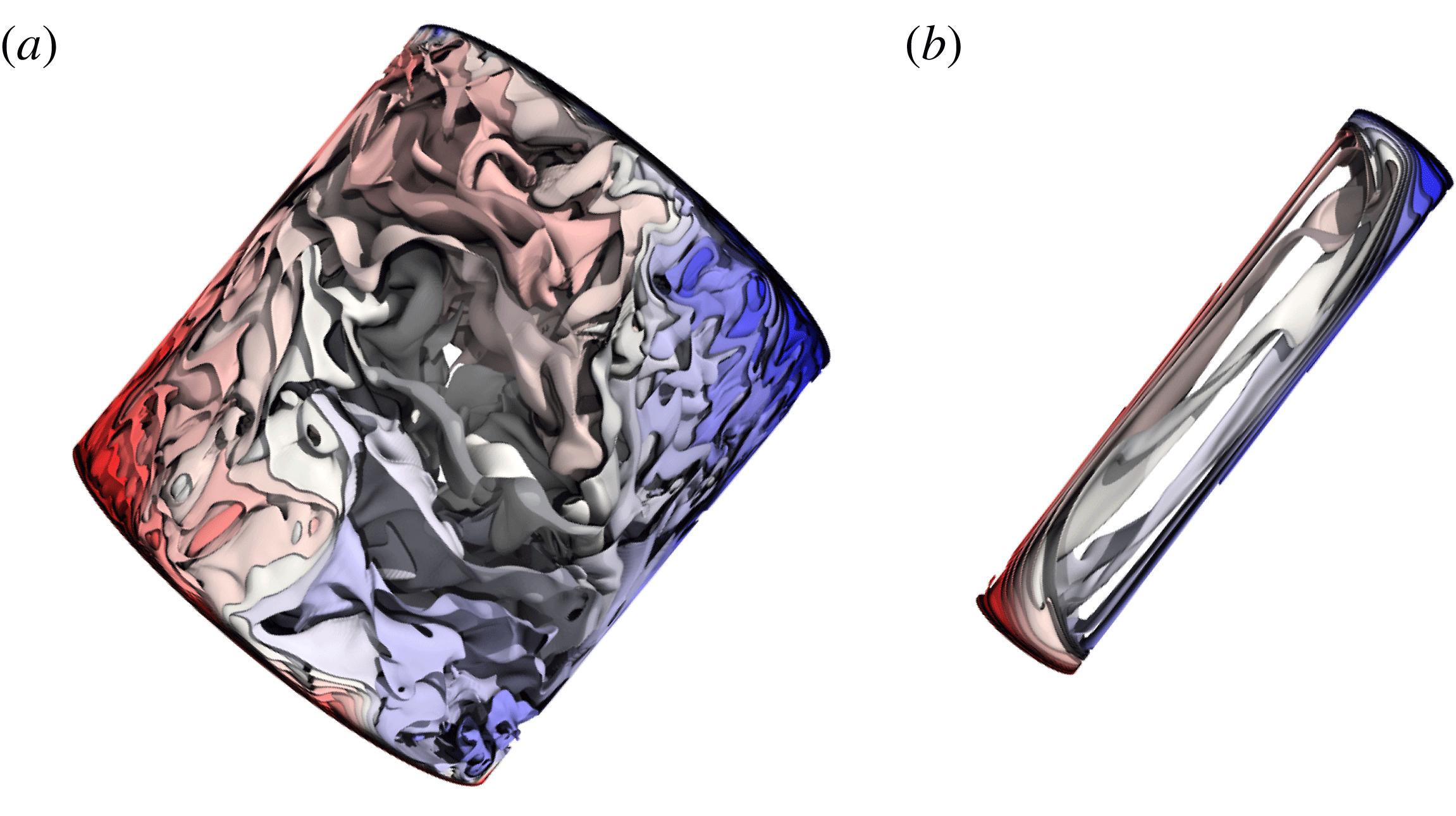
shows just very few. However, the absolute size of the thermal plumes appears to be similar, since the Rayleigh number and Prandtl number are the same for both aspect ratios. Tilting the aspect-ratio-one cylinder causes the plumes to change their orientation with respect to the mean flow direction: they align perpendicular to the streamlines. On the contrary, the optimally inclined, slender cylinder shows no separate thermal plumes, but only one rising and one falling plume, which span the whole cylinder (cf. figures 7
b,e and 13
a,b).
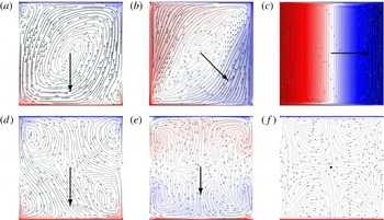
Vertical cross-sections of the time-averaged flow fields, for
 $Ra=10^{9}$
,
 $Pr=1$
and
 $\unicode[STIX]{x1D6E4}=1$
, through (a–c) the plane of the LSC and (d–f) the plane perpendicular to the LSC. The inclination angles are (a,d)
 $\unicode[STIX]{x1D6FD}/\unicode[STIX]{x03C0}=0$
, (b,e)
 $\unicode[STIX]{x1D6FD}=\unicode[STIX]{x03C0}/4$
and (c,f)
 $\unicode[STIX]{x1D6FD}=\unicode[STIX]{x03C0}/2$
. The thick black arrows indicate the strength and direction of gravity. Colour scale and streamlines as in figure 4.

Vertical cross-sections of the time-averaged flow fields, for
 $Ra=10^{9}$
,
 $Pr=1$
and
 $\unicode[STIX]{x1D6E4}=1/5$
, through two perpendicular planes. The inclination angles are (a,b)
 $\unicode[STIX]{x1D6FD}/\unicode[STIX]{x03C0}=0$
, (c,d)
 $\unicode[STIX]{x1D6FD}=\unicode[STIX]{x03C0}/4$
and (e,f)
 $\unicode[STIX]{x1D6FD}=\unicode[STIX]{x03C0}/2$
. Colour scale and streamlines as in figure 4.

Isosurfaces of the instantaneous temperature field for
 $Ra=10^{9}$
,
 $Pr=1$
,
 $\unicode[STIX]{x1D6FD}=\unicode[STIX]{x03C0}/4$
. The aspect ratios are (a)
 $\unicode[STIX]{x1D6E4}=1$
and (b)
 $\unicode[STIX]{x1D6E4}=1/5$
. Colour scale as in figure 4.

Furthermore, the flow inside the slender cylinder is strongly stratified compared to the aspect-ratio-one case (cf. figure 13). In the case of RBC, buoyancy is the only mechanism to cause convection, but as soon as the cell is tilted, the shear flow becomes important. From inclined layer convection, where the aspect ratio is large or infinite, it is known that these are two different instability mechanisms that govern the fluid motion: one due to buoyancy and the other due to shear. The buoyancy or thermal mechanism leads to the development of longitudinal rolls where the axes are aligned with the shear flow. The onset of the longitudinal rolls is independent of
 $Pr$
. The other mechanism, i.e. the shear-flow mechanism, determines the development of transverse rolls, the axes of which are transverse to the shear. In the competition between these two mechanisms, the Prandtl number is crucial: for
 $Pr<0.26$
transverse rolls are always realized, while for larger
 $Pr$
longitudinal rolls may start first if the inclination angle is not too large. This has been studied in various works – see Chen & Pearlstein (Reference Chen and Pearlstein1989), Fujimura & Kelly (Reference Fujimura and Kelly1993), Bodenschatz et al. (Reference Bodenschatz, Pesch and Ahlers2000), Daniels, Plapp & Bodenschatz (Reference Daniels, Plapp and Bodenschatz2000), Daniels, Wiener & Bodenschatz (Reference Daniels, Wiener and Bodenschatz2003) and references therein. Thus, depending on the aspect ratio, there might be a specific inclination angle at which both mechanisms support the heat transport in such a way that it can explain the strong increase of the heat transport in inclined convection.
Further features of the flow become apparent in the time-averaged fields. These are again taken at the edge of the thermal BL,
 $z=\unicode[STIX]{x1D6FF}_{\unicode[STIX]{x1D703}}$
, as horizontal slices (figure 7
g–l). In RBC inside the aspect-ratio-one cell a long-term LSC is present in the flow, as one can see in figures 7(g) and 11(a). In contrast to this, for
 $\unicode[STIX]{x1D6E4}=1/5$
, there are no signs of an LSC visible; instead, there are ring vortices close to the plates (figure 12
a,b). The inclined aspect-ratio-one cell shows a symmetric flow field (figure 7
h) with two hot channels at each side and a smaller impinging zone compared to
 $\unicode[STIX]{x1D6E4}=1/5$
(figure 7
k). For the latter case we observe that the asymmetric flow from the instantaneous field is still present, despite a long averaging time of
 $t_{avg}=1725T_{f}$
. However, the flow is not steady: the velocity is still fluctuating, which means that the asymmetric flow structure prevails for a long time. This asymmetry can be seen in the vertical slice through the plane that is perpendicular to the LSC as well (figure 12
d). In vertical convection the velocity field in the aspect-ratio-one case is almost parallel over the whole plate, although one can see the influence of the sidewalls (figure 7
c,f). In the averaged fields (figures 11
c,f and 12
e,f) we see a difference in the flow organization in the vertical slice that is perpendicular to the LSC. In the small-aspect-ratio case there is only one saddle point in the velocity vector field, while in the aspect-ratio-one case, there are three saddle points at half height.
3.5 Limiting cases: Rayleigh–Bénard and vertical convection
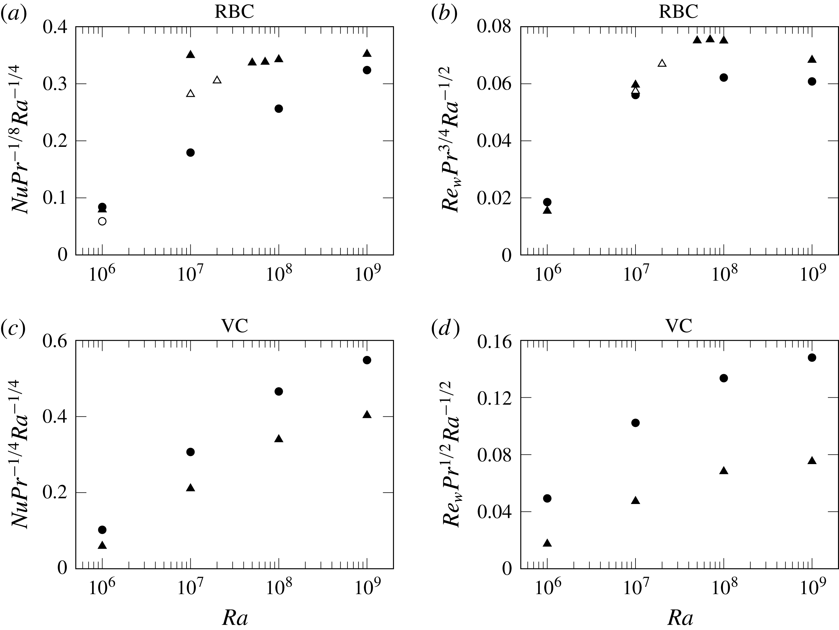
(a,c) The Nusselt number and (b,d) the Reynolds number, compensated with respect to the Rayleigh and Prandtl number scaling relations in the regime
 $I_{l}$
(a,b) in RBC (Grossmann & Lohse Reference Grossmann and Lohse2000) and (c,d) in VC (Shishkina Reference Shishkina2016) for Prandtl numbers
 $Pr=1$
(triangles) and
 $Pr=0.1$
(circles). Flows in a single-roll state are marked with filled symbols and flows in double-roll state are marked with open symbols.

Global heat and momentum transport scaling relations
 $Nu\sim Ra^{a}Pr^{b}$
and
 $Re\sim Ra^{c}Pr^{d}$
, respectively, are of common interest in all configurations of convective flows and here we will briefly discuss the two limiting cases of inclined convection, which are RBC (
 $\unicode[STIX]{x1D6FD}=0$
) and VC (
 $\unicode[STIX]{x1D6FD}=\unicode[STIX]{x03C0}/2$
). The scaling relations for these cases are presented in figure 14 in compensated plots with the scaling exponents according to the boundary-layer-determined low-Prandtl-number regime
 $I_{l}$
(Grossmann & Lohse Reference Grossmann and Lohse2000; Shishkina Reference Shishkina2016). Here the wind-based Reynolds number (2.7) is used, since the GLT assumes a large-scale wind above the BL, which is best represented by the velocity along the plate.
In the regime
 $I_{l}$
, the kinetic and thermal energy dissipation rates are both dominated by their BL contributions. In the vicinity of the plates, the kinetic BL is embedded in the thermal one, while the kinetic BL, which is attached to the adiabatic sidewall of the cylinder, is located outside the thermal BL. In a slender container, the kinetic BL at the adiabatic sidewall occupies a larger fraction of the total volume and this strongly influences the scaling relations.
In all considered cases we observe the exponents (
 $a$
and
 $c$
) in the
 $Nu$
versus
 $Ra$
and in the
 $Re$
versus
 $Ra$
scaling relations, which are larger than those predicted for fully developed, unconfined convective flows. The reason for this discrepancy is the strong lateral geometric confinement (small
 $\unicode[STIX]{x1D6E4}$
) that shifts the onset of convection to higher critical Rayleigh numbers. Since for fully developed convective flows the scaling exponents
 $a$
and
 $c$
should be the same for all
 $\unicode[STIX]{x1D6E4}$
, in the case
 $\unicode[STIX]{x1D6E4}<1$
there exists a transitional
 $Ra$
region with higher scaling exponents than those predicted by the theory for infinite plates. In other words, for the considered Rayleigh numbers, the size of the heated/cooled plates is not sufficiently large to observe the scaling relations proposed for infinite plates. This kind of transition was observed previously, for example in DNS of RBC inside an aspect-ratio-one cylinder, where the onset of convection and the transition to turbulence in mercury were investigated (cf. figure 11 in Verzicco & Camussi (Reference Verzicco and Camussi1997)). The above discussed influence of the geometrical confinement on the scaling relations is stronger for smaller Rayleigh numbers.
Finally we note that, although the obtained exponent
 $a$
in the
 $Nu$
versus
 $Ra$
scaling relation in VC is slightly larger than that proposed in Shishkina (Reference Shishkina2016) (
 $a=1/4$
), it is significantly smaller than that proposed in Castaing et al. (Reference Castaing, Rusaouën, Salort and Chillà2017) for small-Prandtl-number soft-turbulence regime (
 $a=2$
) and significantly larger than that proposed in Castaing et al. (Reference Castaing, Rusaouën, Salort and Chillà2017) for large-Prandtl-number soft-turbulence regime (
 $a=1/5$
).
4 Summary and conclusions
A favourable combination of the Rayleigh number, Prandtl number, aspect ratio and inclination angle can lead to a large increase in heat transport compared to classical Rayleigh–Bénard convection. Among the studied cases the highest relative increase of the heat transport was observed for
 $Ra=10^{7}$
,
 $Pr=0.1$
and an inclination angle of
 $\unicode[STIX]{x1D6FD}=\unicode[STIX]{x03C0}/4$
in an aspect ratio
 $1/5$
cylinder. In this case, the heat transport is increased by a factor of approximately 2.3.
Changes in the flow structure were identified that lead to the significant increase of the heat transport. First, inside a geometrically confined, slender container there is a stronger enhancement of the LSC, which is caused by the shear flow in inclined convection. The large-scale Reynolds number,
 $Re_{U}$
, can be several times larger in inclined convection compared to RBC. Thus, it increases by a factor of approximately 4.5 at the optimal inclination angle compared to no inclination for the slender cylinder and
 $Ra=10^{9}$
and
 $Pr=1$
. In the aspect-ratio-one cylinder, the large-scale Reynolds number increased only by a factor of 1.6, for the same Rayleigh and Prandtl numbers.
Second, inside the slender cylinder with inclination, plumes stack onto each other forming plume columns that eventually reach and impinge on the opposite BL. Since we always observe the optimal heat transport as soon as those plume columns span the whole cylinder, the interaction of the plumes with the opposite BL is certainly important for the heat transport enhancement.
Third, usually at a larger inclination angle than the optimal one, the flow becomes laminar-like or even (almost) steady. We observe this transition to steady flow for all parameters except for the combination of the highest Rayleigh number and the lowest Prandtl number. This transition to steady flow may show oscillatory states, which means that the route to turbulence in inclined convection is similar to that in RBC.
Furthermore, we observe that for lower Prandtl number and/or larger aspect ratio, the optimal heat transport is reached at a larger value of
 $\unicode[STIX]{x1D6FD}/\unicode[STIX]{x03C0}$
. Careful considerations suggest that this is also the case for higher Rayleigh numbers.
Additionally we observed the existence of single- and double-roll states in RBC and confirmed that the double-roll state has indeed less efficient heat transport compared to the single-roll state.
Since in a slender geometry the sidewalls strongly affect the flow, we could not observe the scaling relations expected for convection between infinite plates. Furthermore, the symmetry is broken by the tilt of the cylinder and we observed asymmetric solutions. For turbulent RBC in the slender cylinder we did not find a prevailing LSC as in the aspect-ratio-one cell. However, the presence of the LSC is not that important in RBC, since the heat transport is approximately the same in the
 $\unicode[STIX]{x1D6E4}=1$
and
 $\unicode[STIX]{x1D6E4}=1/5$
cases. This is in conformity with previous results by Ciliberto, Cioni & Laroche (Reference Ciliberto, Cioni and Laroche1996). However, it is important to note that, in inclined convection inside small-aspect-ratio cylinders, the LSC appears to play a very important role for the heat transport. Thus, our data suggest that the highest increase in heat transport for a certain aspect ratio depends not only on the inclination angle but also on the Rayleigh number and Prandtl number.
Acknowledgements
This work is supported by the Priority Programme SPP 1881 Turbulent Superstructures of the Deutsche Forschungsgemeinschaft (DFG) under the grant Sh405/7. O.S. thanks DFG for the support under the grant Sh405/4 – Heisenberg fellowship. The authors acknowledge Leibniz Supercomputing Centre (LRZ) for providing computing time.
Supplementary movies
Supplementary movies are available at https://doi.org/10.1017/jfm.2018.477.