



1 Introduction
Erythrocytes, commonly known as red blood cells (RBCs), are the primary constituent of human blood. Each cell is composed of a viscous liquid drop of haemoglobin solution encapsulated by a thin elastic membrane. As such, these cells fall under the broad class of soft deformable objects, and their behaviour in flow leads to a rich and complex problem of fluid/structure interaction which, despite a great amount of research over several decades, lacks a clear understanding (see, e.g. Freund (Reference Freund2014) and Viallat & Abkarian (Reference Viallat and Abkarian2014) for recent reviews). Early studies, e.g. by Goldsmith & Marlow (Reference Goldsmith and Marlow1972) and Fischer, Stohr-Liesen & Schmid-Schonbein (Reference Fischer, Stohr-Liesen and Schmid-Schonbein1978), have established that in a simple shear flow, an isolated cell exhibits either a rigid-body-like tumbling (TB) or a liquid-drop-like tank treading (TT) in which the cell membrane and the interior fluid rotate while the cell deforms and maintains an inclination with the flow direction. Recent advances in experimental techniques have revealed additional fine dynamics. Abkarian, Faivre & Viallat (Reference Abkarian, Faivre and Viallat2007) observed that during the TT motion, which occurs above a threshold shear stress, the cell axis also oscillates about a mean angle, resulting in a swinging motion (SW) of the cell. In the same study, an intermittent motion consisting of several swinging cycles interrupted by one or multiple tumble(s) was also observed. These observations have spurred complementary research in computational and analytical modelling. The SW dynamics has been predicted by several three-dimensional (3D) computational models for RBCs and RBC-like deformable bodies (e.g. Kessler, Finken & Seifert Reference Kessler, Finken and Seifert2008; Sui et al. Reference Sui, Low, Chew and Roy2008; Bagchi & Kalluri Reference Bagchi and Kalluri2009; Walter, Salsac & Barthes-Biesel Reference Walter, Salsac and Barthes-Biesel2011; Yazdani & Bagchi Reference Yazdani and Bagchi2011, Reference Yazdani and Bagchi2013) and by reduced-order analytical models (e.g. Abkarian et al. Reference Abkarian, Faivre and Viallat2007; Skotheim & Secomb Reference Skotheim and Secomb2007; Kessler, Finken & Seifert Reference Kessler, Finken and Seifert2009; Noguchi Reference Noguchi2009; Abreu & Seifert Reference Abreu and Seifert2012; Gao, Hu & Castaneda Reference Gao, Hu and Castaneda2012). In contrast, the existence of the intermittent dynamics has remained controversial despite the success of reduced-order models in predicting such dynamics (e.g. Abkarian et al. Reference Abkarian, Faivre and Viallat2007; Skotheim & Secomb Reference Skotheim and Secomb2007; Noguchi Reference Noguchi2009; Abreu & Seifert Reference Abreu and Seifert2012). Indeed, many reduced-order models suffer from the drawback of assuming a fixed cell shape, while large deformation is a hallmark of RBCs in flow. Refinement of these models continues to date to improve their reliability by incorporating, e.g. some amount of deformation (Noguchi Reference Noguchi2009, Reference Noguchi2010; Vlahovska et al. Reference Vlahovska, Young, Danker and Misbah2011). Very recently, Cordasco & Bagchi (Reference Cordasco and Bagchi2014) have predicted the intermittent dynamics using, for the first time, a 3D computational model of fully deformable cells.
While there has been a great deal of research on RBC dynamics in steady shear flows, only a handful of studies exists for unsteady flow conditions. In vivo, RBCs are subject to unsteady conditions due to the pulsatile nature of blood flow and the vasomotion of the blood vessels. Nakajima et al. (Reference Nakajima, Kon, Maeda, Tsunekawa and Shiga1990) experimentally studied cell deformation in a sinusoidally varying shear flow, and observed that the deformation during the retarding phase of the imposed flow is higher than that during the accelerating phase. Watanabe et al. (Reference Watanabe, Kataoka, Yasuda and Takatani2006) also experimentally studied cell deformation at high shear stress and in a low-frequency range (1–5 Hz). They observed that the deformation response lagged behind the imposed shear stress by an amount that was independent of the forcing frequency. The authors also found that the maximum deformation was less than that of a cell subjected to a steady shear flow of the same strength. Using a reduced-order model, and supported by experiments, Dupire, Abkarian & Viallat (Reference Dupire, Abkarian and Viallat2010), hereafter referred to as DAV, showed that the cells could perform either a regular periodic motion or chaotic dynamics. In the periodic motion, the cell reversed its orientation in response to the flow reversals either by passing through the horizontal (flow direction) axis or by passing through the vertical (flow gradient) axis. The chaotic dynamics was manifested as a non-periodic sequence of horizontal and vertical reversals, and was proposed to occur near the resonance of flow frequency and the natural frequency of the cell. A resonant behaviour was also predicted by Kessler et al. (Reference Kessler, Finken and Seifert2009) using a reduced-order model. By including a phenomenological model of cell deformation, Noguchi (Reference Noguchi2010) predicted similar non-periodic dynamics to those observed by DAV in certain ranges of oscillation frequency, and periodic reversals at low frequencies. Additionally, he found that multiple limit cycles were possible at high frequency depending on the initial conditions.
Computational studies of RBC dynamics in oscillating shear flow using direct 3D models of fully deformable cells or cell-like bodies have been rare. Zhao & Bagchi (Reference Zhao and Bagchi2011) considered capsules of resting ellipsoidal and spherical shapes in sinusoidally oscillating shear flow and observed rigid-body-like orientation reversals at low shear rates and deformation-driven reversals at high shear rates. The authors further noted that the dynamics was highly sensitive to the initial conditions, suggesting the possibility of chaos. Matsunaga et al. (Reference Matsunaga, Imai, Yamaguchi and Ishikawa2015) considered spherical capsules subjected to oscillating shear flows and observed a large overshoot in time-dependent deformation compared with a steady shear flow. However, neither Zhao & Bagchi (Reference Zhao and Bagchi2011) nor Matsunaga et al. (Reference Matsunaga, Imai, Yamaguchi and Ishikawa2015) considered the resting biconcave discocyte shape of the RBC in their models. Furthermore, both Zhao & Bagchi (Reference Zhao and Bagchi2011) and Matsunaga et al. (Reference Matsunaga, Imai, Yamaguchi and Ishikawa2015) assumed that the initial shape of the capsule was stress-free, while the model of Matsunaga et al. (Reference Matsunaga, Imai, Yamaguchi and Ishikawa2015) lacked membrane bending resistance which is needed to generate a stress-free state that is different from the resting shape. The notion that the resting biconcave shape is not the stress-free state of the RBC has gained much credence due to several recent studies, e.g. by Dupire, Socol & Viallat (Reference Dupire, Socol and Viallat2012), Li, Vlahovska & Karniadakis (Reference Li, Vlahovska and Karniadakis2013), Tsubota, Wada & Liu (Reference Tsubota, Wada and Liu2013) and Peng, Mashayekh & Zhu (Reference Peng, Mashayekh and Zhu2014). Cordasco & Bagchi (Reference Cordasco and Bagchi2014) showed that the intermittent dynamics of the cells observed in steady shear flow experiments, as well as predicted by reduced-order models, could also be predicted by 3D computational models of fully deformable cells if the stress-free state was assumed to be an oblate spheroid. Zhao & Bagchi (Reference Zhao and Bagchi2011) and Matsunaga et al. (Reference Matsunaga, Imai, Yamaguchi and Ishikawa2015) did not predict many interesting dynamics, such as the occurrence of chaos and the presence of multiple stable limit cycles, that were observed in experiments performed using RBCs in oscillating shear flows and predicted by the reduced-order models by DAV and Noguchi (Reference Noguchi2010). Evidently, our understanding of the RBC dynamics in oscillatory shear flow requires further improvement.
In this article, we present a 3D computational study of fully deformable RBCs of the biconcave resting shape with an appropriate stress-free state as they are subjected to a sinusoidally oscillating shear flow. We provide a comprehensive investigation of the cell dynamics and an analysis over a wide range of flow frequency, shear rate amplitude and viscosity contrast between internal and external fluids. Our study provides the first conclusive evidence of the chaotic dynamics of the cells in oscillating flow, as observed in experiments and predicted by reduced-order models, but using a fully deformable and deterministic cell model without the introduction of any stochastic noise. We further show that chaos is suppressed at higher shear rates due to a large deformation experienced by the cells. Therefore, while our full model confirms the earlier findings at low shear rates, it also underscores the important role that the cell deformation plays at higher shear rates. Specifically, we show that the cell deformation is much larger and is manifested in the form of more complex shapes in oscillating shear flows when compared with steady shear flows of a similar strength.
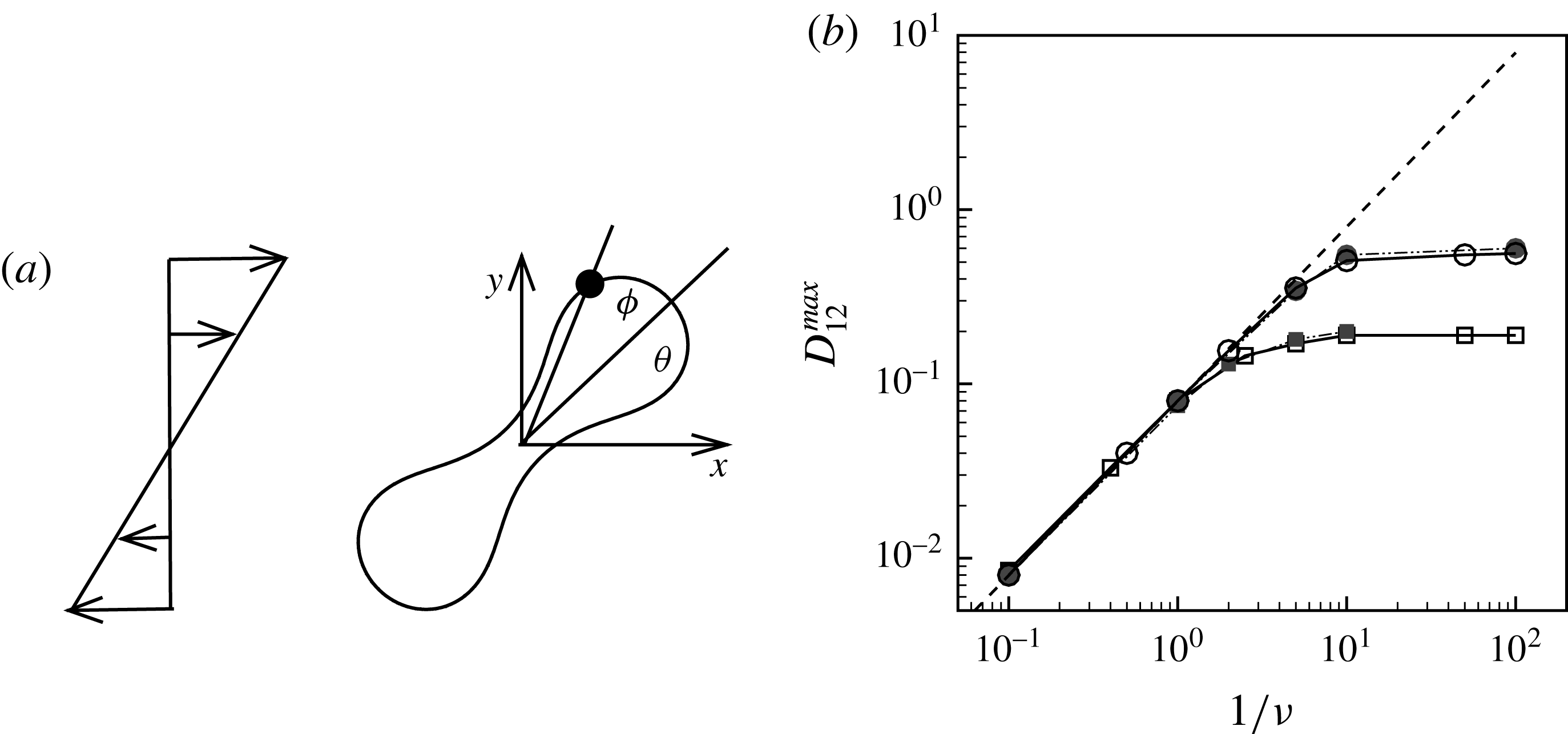
(a) Schematic of an RBC of the biconcave resting shape subjected to a sinusoidally oscillating zero-mean linear shear flow. The angles
 ${\it\theta}$
and
 ${\it\phi}$
are the major axis inclination with respect to the flow direction, and the membrane phase. (b) Comparison of the numerical results (symbols) and the exact analytical result (dashed line) of Matsunaga et al. (Reference Matsunaga, Imai, Yamaguchi and Ishikawa2015) for a spherical capsule in oscillating shear flow. The analytical result is valid in the limit of high
 ${\it\nu}$
. The filled symbols are the present numerical simulations, and the unfilled symbols are from Matsunaga et al. (Reference Matsunaga, Imai, Yamaguchi and Ishikawa2015): ▫,
 $Ca=0.1$
; ○,
 $Ca=1$
;
 ${\it\lambda}=1$
in all cases.
2 Numerical method and problem set-up
We perform 3D numerical simulations of deformable RBCs suspended in a sinusoidally oscillating zero-mean simple shear flow
 $\boldsymbol{u}=\{\dot{{\it\gamma}}y,0,0\}$
, where
 $$\begin{eqnarray}\dot{{\it\gamma}}(t)=\dot{{\it\gamma}}_{a}\sin (2{\rm\pi}\tilde{{\it\nu}}t)\end{eqnarray}$$
is the instantaneous shear rate,
 $t$
is time,
 $\dot{{\it\gamma}}_{a}$
is the amplitude and
 $\tilde{{\it\nu}}$
is the frequency. The axis of revolution of the RBC lies in the shear plane (figure 1). The numerical methodology is described in detail in our previous work, e.g. Yazdani & Bagchi (Reference Yazdani and Bagchi2013) and Cordasco & Bagchi (Reference Cordasco and Bagchi2014). Here, we provide a summary of the method for the sake of completeness. The cell is modelled as a viscous liquid drop enclosed by a zero-thickness elastic membrane having the experimentally observed biconcave discocyte shape as the resting shape. The interior and suspending fluids are assumed to be incompressible and Newtonian with viscosity
 ${\it\lambda}{\it\mu}_{o}$
and
 ${\it\mu}_{o}$
respectively. The membrane is assumed to possess a resistance against shear deformation, area dilatation and bending. The shear deformation and area dilatation are modelled following Skalak et al. (Reference Skalak, Tozeren, Zarda and Chien1973) using an in-plane strain energy function as
 $$\begin{eqnarray}W_{E}=\frac{G_{s}}{4}[(I_{1}^{2}+2I_{1}-2I_{2})+CI_{2}^{2}],\end{eqnarray}$$
where
 $G_{s}$
is the membrane shear elastic modulus,
 $I_{1}={\it\epsilon}_{1}^{2}+{\it\epsilon}_{2}^{2}-2$
and
 $I_{2}={\it\epsilon}_{1}^{2}{\it\epsilon}_{2}^{2}-1$
are the strain invariants of the Green strain tensor, and
 ${\it\epsilon}_{1}$
and
 ${\it\epsilon}_{2}$
are the principal stretch ratios. The parameter
 $C$
limits the surface area dilatation. The area dilatation of an RBC is nearly zero; this requires the use of a very high value of
 $C$
which leads to numerical instability. Based on our previous extensive numerical experiments (e.g. Yazdani & Bagchi Reference Yazdani and Bagchi2011; Cordasco, Yazdani & Bagchi Reference Cordasco, Yazdani and Bagchi2014), we found that
 $C=1000Ca$
limits the surface area change without causing a numerical instability. Hence, this is the value of
 $C$
used in the present study. However, this expression of
 $C$
should not be used to infer that it is the area dilatation modulus. A finite-element method is used to obtain the membrane tension resulting from the shear deformation and area dilatation. The bending resistance is modelled following Helfrich’s formulation for bending energy (Zhong-can & Helfrich Reference Zhong-can and Helfrich1989),
 $$\begin{eqnarray}W_{B}=\frac{E_{b}}{2}\int _{S}(2{\it\kappa}-c_{o})^{2}\,\text{d}S,\end{eqnarray}$$
where
 $E_{b}$
is the bending modulus,
 ${\it\kappa}$
is the mean curvature,
 $c_{o}$
is the spontaneous curvature and
 $S$
is the surface area. An expression for a bending force density derived from (2.3) was used in the numerical implementation. The fluid motion interior and exterior to the cell is obtained by solving the Navier–Stokes equations with negligible inertia. A combination of spectral and finite-difference schemes is used for the flow solver. The coupling between the flow and the membrane deformation is performed using a front-tracking/immersed-boundary method. The computational domain is a cubic box of length
 $2{\rm\pi}a_{o}$
, where
 $a_{o}$
is the radius of a sphere having the same volume as the cell. The domain is discretized by
 $120^{3}$
points, and the cell surface is discretized using 20 480 triangular elements. The dimensionless time is denoted by
 $t^{\ast }=t\dot{{\it\gamma}}_{a}$
.
The relevant dimensionless parameters for the present study are the ratio of the peak viscous force to the membrane elastic force
 $Ca=\dot{{\it\gamma}}_{a}\,{\it\mu}_{o}\,a_{o}/G_{s}$
, the viscosity ratio
 ${\it\lambda}$
and the dimensionless frequency of the flow oscillation
 ${\it\nu}=\tilde{{\it\nu}}/\dot{{\it\gamma}}_{a}$
. The ranges of
 $Ca$
and
 ${\it\lambda}$
considered here are 0.03–0.5 and 0.1–5 respectively, corresponding to a shear rate of approximately 0.3–
 $300~\text{s}^{-1}$
. The shear rate is typical of a microcirculatory flow, and the physiological
 ${\it\lambda}$
is approximately 5. The dimensionless frequency range considered is
 $1/{\it\nu}=5{-}120$
.
The stress-free state of the cell is assumed to be an oblate spheroid of reduced volume
 $V_{0}=V_{obl}/(A^{3/2}/3\sqrt{4{\rm\pi}})=0.997$
, where
 $V_{obl}$
is the spheroid volume and
 $A=134.1~{\rm\mu}\text{m}^{2}$
is the surface area of a normal RBC. The biconcave resting shape is generated numerically from the spheroid by deflation until the desired volume
 $V_{cell}=94.1~{\rm\mu}\text{m}^{3}$
of a normal RBC is reached. The cell deflation is obtained by imposing a small inward velocity normal to the membrane starting from a quasi-spherical oblate of reduced volume 0.997 but with its surface area the same as that of a normal RBC. The solution is unique and is a function of the spontaneous curvature and dimensionless bending stiffness. The numerical scheme is stable as long as a sufficiently small deflation velocity is used. Further details on the deflation process were given in Cordasco et al. (Reference Cordasco, Yazdani and Bagchi2014). The final shape agrees well with the experimental shape as given in Fung (Reference Fung1993) and has a reduced volume of 0.644, the same as that of a normal RBC. From numerical experiments we find that
 $c_{0}=4.0$
gives the experimental shape. It should be emphasized that the resting biconcave shape is generated under the balance of membrane shear resistance and bending resistance. The membrane shear modulus and bending stiffness used in the simulations are approximately
 $2.5\times 10^{-6}~\text{N}~\text{m}^{-1}$
and
 $6\times 10^{-19}$
J respectively.
The cell dynamics is identified using two angles within the shear plane: the inclination angle
 ${\it\theta}$
of the RBC major axis with respect to the flow direction and the phase angle
 ${\it\phi}$
of a marker point on the cell surface with respect to the long axis of the cell (figure 1). For a full TT,
 ${\it\phi}$
is displaced by
 $2{\rm\pi}$
. In a steady shear flow, TT can be accompanied by an SW, in which case
 ${\it\theta}$
oscillates about a mean, and the SW period is half of the TT period. For a tumble,
 ${\it\phi}$
oscillates about a mean, but
 ${\it\theta}$
varies by
 $2{\rm\pi}$
in a full rotation. The initial inclination angle is denoted by
 ${\it\theta}_{o}$
. The volume of the cell is preserved; the total change in cell volume is less than 0.1 % (see Cordasco & Bagchi (Reference Cordasco and Bagchi2014) and the supplementary material therein for details).
Comparison of our numerical results with the exact analytical result and numerical results of Matsunaga et al. (Reference Matsunaga, Imai, Yamaguchi and Ishikawa2015) is shown in figure 1(b). Matsunaga et al. extended the small-deformation theory of Barthes-Biesel & Rallison (Reference Barthes-Biesel and Rallison1981) in the limit of high
 ${\it\nu}$
. The maximum Taylor deformation parameter was predicted to be
 $D_{12}^{\mathit{max}}=5/(4{\rm\pi}{\it\nu}(2{\it\lambda}+3))$
. The numerical results agree well with the analytical result at the high-
 ${\it\nu}$
limit. The two results deviate at lower frequencies, with the numerical results becoming less sensitive to
 ${\it\nu}$
, as also noted by Matsunaga et al. (Reference Matsunaga, Imai, Yamaguchi and Ishikawa2015). Additionally, our numerical results at lower frequencies also agree very well with the numerical results of Matsunaga et al. (Reference Matsunaga, Imai, Yamaguchi and Ishikawa2015).
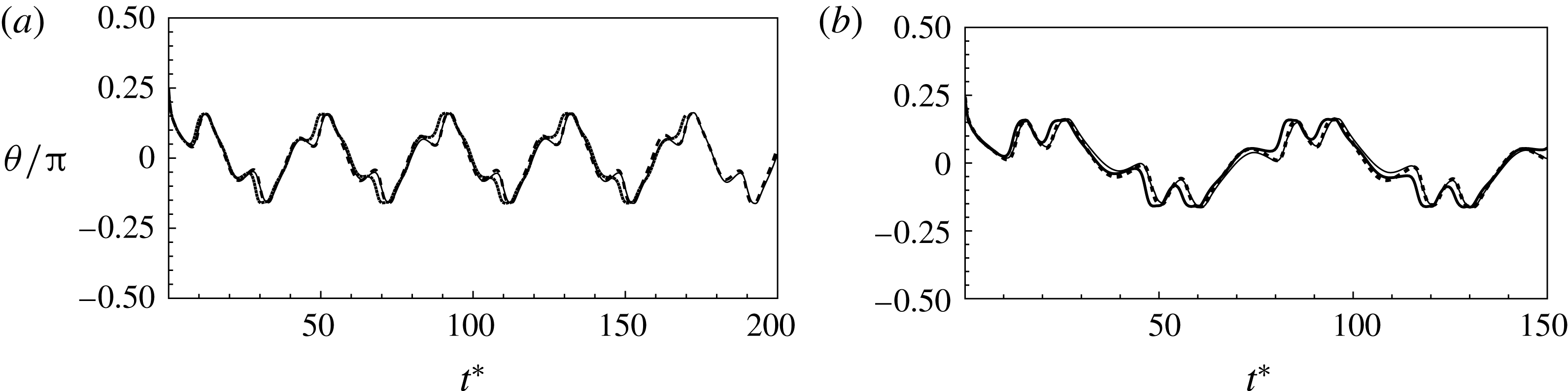
To illustrate that the RBC dynamics observed here are not numerical artefacts, we present a grid and domain size independence study. The grid independence is tested by considering three different Eulerian resolutions as
 $120^{3}$
,
 $180^{3}$
and
 $240^{3}$
, and two different Lagrangian resolutions as 20 480 and 49 152 triangular elements on the cell surface. Figure 2(a,b) shows two sample cases for which periodic oscillatory dynamics is observed. Trajectories for different resolutions are observed to coincide, and therefore grid independence is established for periodic dynamics. The influence of domain size is tested by doubling the domain size. The results are presented in figure S1 in the supplementary material available at http://dx.doi.org/10.1017/jfm.2016.409. For the regular periodic dynamics as shown in S1(a–c), there is nice overlap in the results for the two domains.
The grid and domain size effects on the chaotic dynamics are presented later in § 3.1.2.
Grid convergence tests. The continuous lines are for
 $120^{3}$
Eulerian and 20 480 Lagrangian resolutions, the dashed lines are for
 $180^{3}$
and 49 152, and the dotted lines are for
 $240^{3}$
and 49 152. Panels (a) and (b) consider two examples taken from regular periodic dynamics.
3 Results and discussion
3.1 Dynamical behaviour
Simulations are performed over a wide range of
 $Ca$
,
 ${\it\lambda}$
and
 ${\it\nu}$
. Often, the dynamics is dependent on the initial orientation angle
 ${\it\theta}_{o}$
, which is also varied. Generally, the cell dynamics is observed to be either periodic or chaotic. In what follows, we first illustrate the dynamics under varying
 ${\it\nu}$
, followed by some analysis of the chaotic dynamics. Then, the influence of viscosity ratio, shear rate and cell deformation is considered.
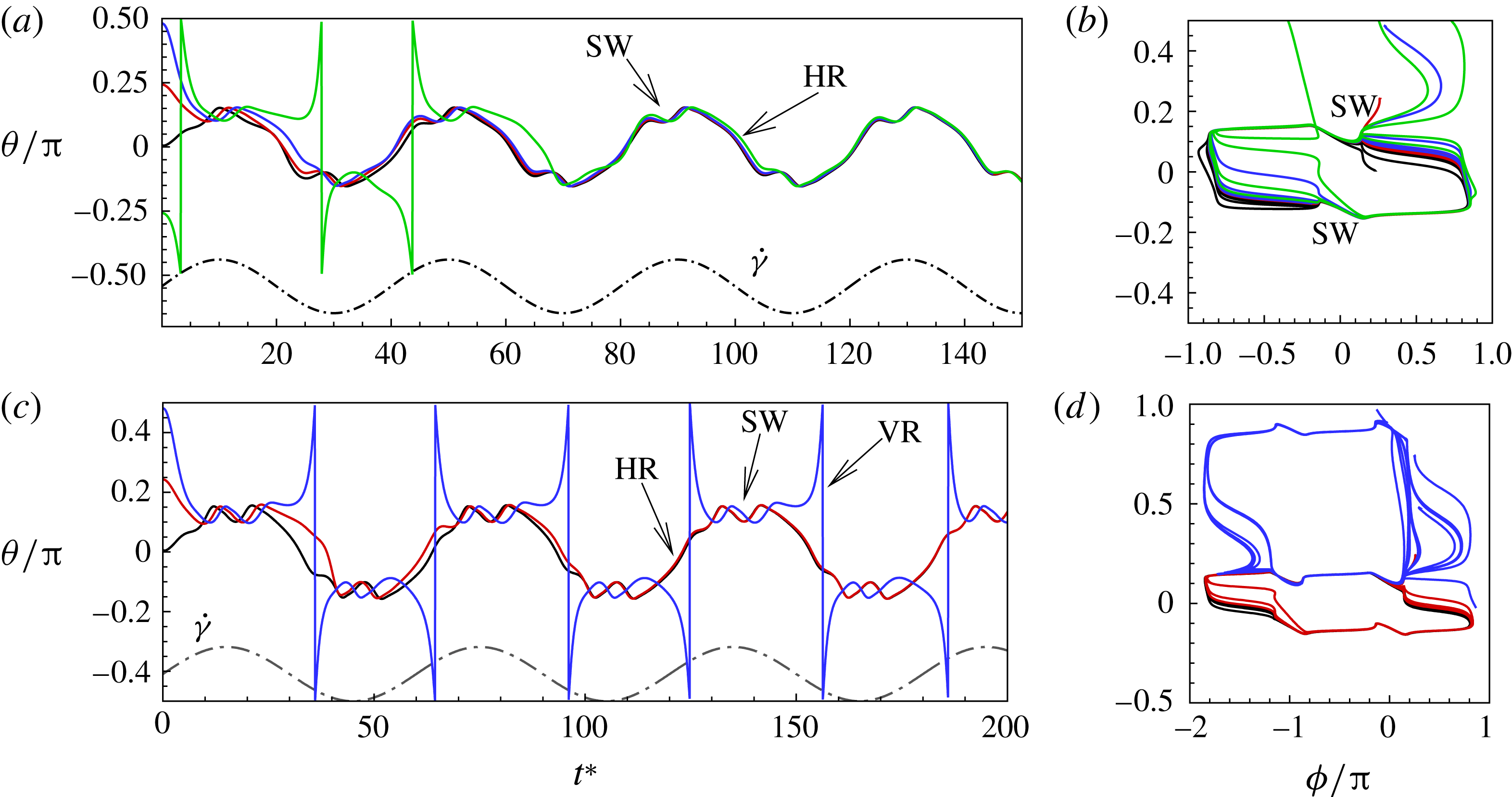
Cell dynamics at high dimensionless frequency (
 $1/{\it\nu}=5$
,
 $Ca=0.04$
,
 ${\it\lambda}=0.85$
). (a) Time history of cell inclination
 ${\it\theta}$
for various initial orientations as
 ${\it\theta}_{o}=0$
(black),
 ${\rm\pi}/4$
(red),
 ${\rm\pi}/2$
(blue),
 $3{\rm\pi}/4$
(green). Horizontal reversals (HRs) occur for
 ${\it\theta}_{o}=0$
and
 ${\rm\pi}/4$
, and vertical reversals (VRs) occur for
 ${\it\theta}_{o}={\rm\pi}/2$
and
 $3{\rm\pi}/4$
. (b) The
 ${\it\theta}$
–
 ${\it\phi}$
phase-space plot showing the limit cycles associated with HRs (black and red) and VRs (green and blue). (c,d) Snapshots from our simulations showing VRs and HRs respectively over one half flow cycle for
 $1/{\it\nu}=30$
,
 $Ca=0.1$
,
 ${\it\lambda}=0.1$
. The major axis of the cell oscillates about the flow gradient (
 $y$
) axis in VRs and about the flow direction (
 $x$
-axis) in HRs. Animations are provided as supplementary movies 1 and 2.

3.1.1 Periodic dynamics
The cell dynamics at high
 ${\it\nu}$
is shown in figure 3 where
 $1/{\it\nu}=5$
is considered. At such high
 ${\it\nu}$
, the dynamics is observed to be periodic, but dependent on the initial orientation
 ${\it\theta}_{o}$
. Cells settle into a back-and-forth motion: the cell major axis oscillates either about the flow direction (
 $x$
-axis,
 ${\it\theta}=0$
) or about the flow gradient axis (
 $y$
-axis,
 ${\it\theta}={\rm\pi}/2$
). The former is termed as horizontal reversal (hereafter referred to as HR) and the latter as vertical reversal (VR). For some
 ${\it\theta}_{o}$
, the initial conditions can be felt for a long time before the cells settle into either of the two periodic motions.
Representative snapshots of VRs and HRs are shown in figures 3(c) and 3(d) respectively for a half flow cycle. Animations are provided as supplementary movies. For a VR, the cell rotates in the same direction as the flow rotation with almost no phase lag with respect to the flow. The cell crosses the vertical axis during the flow acceleration to orient its axis from the compressional to the extensional direction, and remains aligned in the extensional quadrant during the deceleration phase. In contrast, for an HR, there is a large phase lag, and the cell may rotate in a direction opposite to the flow rotation.
The oscillation of the whole cell is accompanied by a back-and-forth motion of the cell membrane. The combined motion can be described by a phase-space plot in terms of
 ${\it\theta}$
and
 ${\it\phi}$
, as shown in figure 3(b). In this plot, the HRs and VRs appear as two distinct non-intersecting limit cycles. The occurrence of two limit cycles was reported earlier by DAV in their experiments and reduced-order modelling. Here, we successfully capture these limit cycles using a 3D fully deformable cell model.
Figure 3 also shows that the cell sweeps a larger angle while in a VR than in an HR. As will be shown later, this difference has a significant effect on the appearance of the chaotic dynamics and also on the cell deformation in oscillating flow. In contrast, the amount of membrane displacement is less in a VR than in an HR. This is because the cell experiences a higher torque while in the vertical orientation; since a part of the torque is also used to displace the cell membrane, a larger variation in
 ${\it\phi}$
occurs in an HR. Furthermore, in an HR, a greater amount of membrane movement occurs when cell rotation and flow rotation are in opposite directions than when they are in the same direction.
The results in figure 3 are for
 $Ca=0.04$
and
 ${\it\lambda}=0.85$
, for which cell deformation is small, and, hence, the dynamics can be clearly illustrated. The effect of cell deformation is given in a later section.
Although deformation is small and inertia is negligible, the coalescing trajectories presented in figure 3, and also in subsequent figures, represent a major difference between the dynamics of an RBC and a rigid ellipsoid. It is well known from Jeffery’s (Reference Jeffery1922) solution that a rigid axisymmetric ellipsoid in an oscillating shear flow would result in an infinite number of non-coalescing trajectories that are dependent on the initial orientation. Chaotic rotation is, however, possible for long triaxial ellipsoidal particles (Yarin, Gottlieb & Roisman Reference Yarin, Gottlieb and Roisman1997).
The effect of decreasing the dimensionless frequency,
 $1/{\it\nu}=22$
: (a,b) H-entrainment,
 $Ca=0.04$
,
 ${\it\lambda}=0.85$
,
 ${\it\theta}_{o}=0$
(red line),
 ${\rm\pi}/6$
(green),
 ${\rm\pi}/2$
(black),
 $5{\rm\pi}/6$
(blue); (c,d) non-coalescing HR,
 $Ca=0.1$
,
 ${\it\lambda}=0.3$
,
 ${\it\theta}_{o}=44{\rm\pi}/180$
(solid black line),
 $45{\rm\pi}/180$
(solid red),
 $46{\rm\pi}/180$
(solid blue),
 $-44{\rm\pi}/180$
(solid green),
 $-45{\rm\pi}/180$
(dashed black),
 $-46{\rm\pi}/180$
(dash–dot red).

Decreasing the dimensionless frequency has a profound effect on the cell dynamics. As
 $1/{\it\nu}$
is gradually increased from 5, a VR becomes unstable and transforms to an HR. At
 $1/{\it\nu}=22$
, as shown in figure 4(a,b), the initial conditions are completely forgotten and the cells settle into one trajectory exhibiting only the HR. Consequently, in
 ${\it\theta}$
–
 ${\it\phi}$
phase space, trajectories with different initial conditions merge into a single stable limit cycle. Such a behaviour is known as frequency entrainment in the study of forced nonlinear oscillators (Jordan & Smith Reference Jordan, Smith, Jordan and Smith2007), and is closely related to the synchronization or mode-locking phenomenon. Here, we identify such dynamics as H-entrainment.
For a certain range of parameters, we observe that cells with different initial conditions settle into HR, but their trajectories do not coalesce anymore. Such cases are shown in figure 4(c,d), where it can be noticed that even small differences in the initial conditions result in clearly different but stable trajectories. Consequently, the
 ${\it\theta}$
–
 ${\it\phi}$
phase plot shows multiple stable but non-coalescing attractors of similar shape and locations. Such multiple stable limit cycles were predicted by the reduced-order model of Noguchi (Reference Noguchi2010). Interestingly, figure 4(c,d) shows that cells with small differences in their initial conditions exhibit distinctly different trajectories with non-periodic dynamics during the initial part of the simulations, but eventually settle into a periodic HR. As will be shown later, in a particular parameter range, the non-periodic behaviour continues over a long time resulting in chaotic dynamics.
The effect of decreasing
 ${\it\nu}$
: (a,b)
 $1/{\it\nu}=40$
; the dynamics appears as an H-entrainment with SWs occurring near the peak shear rate; (c,d)
 $1/{\it\nu}=60$
; multiple SWs occur along with VRs or HRs depending on
 ${\it\theta}_{o}$
. For all panels,
 $Ca=0.1$
,
 ${\it\lambda}=0.1$
;
 ${\it\theta}_{o}=0$
(black),
 ${\rm\pi}/4$
(red),
 ${\rm\pi}/2$
(blue),
 $-{\rm\pi}/4$
(green).
The dynamics with HRs continues as
 ${\it\nu}$
is further reduced. At sufficiently reduced
 ${\it\nu}$
, the dynamics appears as a combination of SWs and HRs. A swing occurs when the instantaneous shear rate
 $\dot{{\it\gamma}}$
is greater than the threshold shear rate for the TB–TT transition in a steady shear flow, and an HR occurs when
 $\dot{{\it\gamma}}$
is less than the threshold. Such cases are shown in figure 5(a,b) for
 $1/{\it\nu}=40$
. Also noticeable here is the entrainment of different trajectories into a horizontal limit cycle. When
 ${\it\nu}$
is reduced even further, e.g. for
 $1/{\it\nu}=60$
as shown in figure 5(c,d), multiple swings are possible near the peak shear rate. Furthermore, both VRs and HRs now emerge depending on
 ${\it\theta}_{o}$
.
Angular oscillation amplitude
 ${\rm\Delta}{\it\theta}$
as a function of
 ${\it\nu}$
for
 ${\it\lambda}=0.1$
(▫) and 1 (▵). Here,
 $Ca=0.1$
is constant. Simulation results are shown by continuous lines and filled symbols, while the DAV model is shown by dotted lines and unfilled symbols.

It is of interest to quantitatively compare the results from our simulation and the DAV model. Since the latter is for shape-preserving cells, we restrict the comparison to
 $Ca=0.1$
for which the deformation is not large. To obtain the results for the DAV model, we use the same parameters as used in their paper. The values of
 $Ca$
used in the simulations are converted to dimensional shear rates using the definition of
 $Ca$
and the values of
 $G_{s}$
and
 $a_{o}$
as given in § 2. The dimensional frequency in the DAV model is also related to the dimensionless frequency as noted in § 2. The quantity of interest is the amplitude of angular oscillation
 ${\rm\Delta}{\it\theta}$
, which is plotted in figure 6 as a function of
 ${\it\nu}$
. Keeping in mind the limitations of the DAV model, it can be said that good agreement between the model and our simulation is observed at low shear rates. Additionally, both the DAV model and the simulation predict higher
 ${\rm\Delta}{\it\theta}$
in VRs than in HRs. Furthermore, with decreasing
 ${\it\nu}$
,
 ${\rm\Delta}{\it\theta}$
first increases but then saturates. At high
 ${\it\nu}$
,
 ${\rm\Delta}{\it\theta}$
is restricted by flow oscillation. At very low
 ${\it\nu}$
, SW occurs over longer times. The maximum inclination of the cell is then limited by SW as in a steady shear flow, resulting in the observed saturation of
 ${\rm\Delta}{\it\theta}$
.
3.1.2 Chaotic dynamics
As noted in the introduction, in their experiments, DAV first observed that RBCs exhibited chaotic behaviour. As opposed to the periodic dynamics presented in the last section, the chaotic dynamics is characterized by an irregular (i.e. non-periodic) sequence of horizontal reversals, vertical reversals and swinging of the cells. In experiments, usually many factors are present including thermal and background noise that may cause such chaotic motion to occur. It is of interest, therefore, to investigate whether chaotic motion occurs in the absence of such external noise. Similar chaotic dynamics is observed in our simulations, as shown in figure 7(a). An SW occurs near the peak
 $\dot{{\it\gamma}}$
, and VRs and HRs occur near the instances of flow reversals, as is evident in the close-up view shown in figure 7(b). In order to investigate whether the observed aperiodic trajectories are indicative of chaotic dynamics, we consider five simulations with very close
 ${\it\theta}_{o}$
(differing by one degree or less) and let the motion evolve for a long time. Although chaotic dynamics arises from a fully deterministic set of equations as is the case in our simulations, it is highly sensitive to the initial conditions and should exhibit a diverging behaviour with even small variations in initial conditions. As is evident in the time series plots in figure 7(c), the trajectories are nearly identical during the early time in the simulations, but they begin to diverge after several flow reversal cycles. Eventually, the trajectories become widely different from each other. This is indeed a signature of a chaotic regime encountered in deterministic nonlinear systems. It is also observed that two trajectories can nearly coincide in some time intervals, while they can be widely apart at other times. This is also a well-known characteristic of so-called strange attractors.
Chaotic dynamics,
 $Ca=0.1$
,
 ${\it\lambda}=0.1$
,
 $1/{\it\nu}=22$
; (a)
 ${\it\theta}$
versus
 $t^{\ast }$
showing the aperiodic behaviour for different initial orientations
 ${\it\theta}_{o}=0$
(black),
 ${\rm\pi}/4$
(red),
 ${\rm\pi}/2$
(blue),
 $-{\rm\pi}/4$
(green); (b) close-up of two cases shown in (a); the cell dynamics is an irregular sequence of SWs, VRs and HRs; (c)
 ${\it\theta}$
versus
 $t^{\ast }$
showing widely diverging trajectories resulting from small differences in
 ${\it\theta}_{o}$
as 0 (black),
 ${\rm\pi}/1800$
(blue),
 $-{\rm\pi}/1800$
(green),
 ${\rm\pi}/180$
(magenta),
 $-{\rm\pi}/180$
(red). The arrow indicates where the trajectories start to diverge.

We now establish the grid and domain size independence for the chaotic dynamics, as shown in figure 8. We consider
 $180^{3}$
Eulerian resolution and 49 152 Lagrangian resolution, and
 $240^{3}$
Eulerian resolution and 49 152 Lagrangian resolution respectively. The results with
 $120^{3}$
Eulerian resolution and 20 480 Lagrangian resolution have already been given in figure 7. As noted before, the chaotic trajectories are characterized by aperiodic and irregular sequences of HRs, VRs and SWs. The chaotic trajectories are evident at higher resolutions as well. Further, for small differences in initial orientations, widely divergent trajectories are observed for all resolutions, which is also another indication of chaos.
The domain size independence for the chaotic dynamics is shown in figure S1(d) in the supplementary material, clearly establishing that both the original and the increased domains show chaotic trajectories.
Grid convergence test for the chaotic dynamics. The dashed lines are for
 $180^{3}$
Eulerian resolution and 49 152 Lagrangian resolution, and the dotted lines for
 $240^{3}$
and 49 152. The colours indicate different initial orientations as in figure 7. Here, only the trajectories for
 $180^{3}$
and
 $240^{3}$
are plotted to avoid clutter. The trajectories for
 $120^{3}$
Eulerian resolution and 20 480 Lagrangian resolution have already been given in figure 7. Trajectories at higher resolutions show similar irregular aperiodic behaviour to that shown in figure 7. It should be noted that for the chaotic dynamics, the trajectories should not coincide for two different resolutions as this is the fundamental nature of chaotic dynamics.

Further support for the existence of chaos is obtained by considering additional simulations where the sensitivity to other parameters, namely
 $Ca$
,
 ${\it\lambda}$
and
 ${\it\nu}$
, is considered with small differences. Again, small variations of these parameters lead to widely different trajectories over a long time. These results are not presented for brevity.
The
 ${\it\theta}{-}{\it\phi}$
phase plot for the chaotic dynamics is shown in figure 9(a), which appears as an irregular sequence of vertical and horizontal attractors in the form of staircases. Over certain time windows, a clockwise or counterclockwise rotation of the cell is possible; however, over a long time, no preference in rotational direction exists. A close-up of the phase plot is shown in figure 9(b), which demonstrates that SWs appear as inflections at the top left and bottom right corners of the H-attractors where the vertical and horizontal limit cycles intersect. Therefore, the bifurcation between the vertical and horizontal limit cycles occurs via a swing. It should be noted that for the periodic dynamics, e.g. as shown previously in figure 3(a), the vertical and horizontal attractors do not intersect. The intersection of V- and H-attractors in the phase space is fundamental to the emergence of the chaotic dynamics, and will be further elucidated.
Chaotic dynamics: (a)
 ${\it\theta}$
–
 ${\it\phi}$
phase plot for the trajectories shown in figure 7 illustrating irregular sequences of V- and H-attractors; (b) a close-up of a part of a trajectory in (a) showing that bifurcation occurs via a swing; (c) attractors are plotted together by shifting in
 ${\it\theta}$
and
 ${\it\phi}$
, showing dense trajectories characteristic of strange attractors.
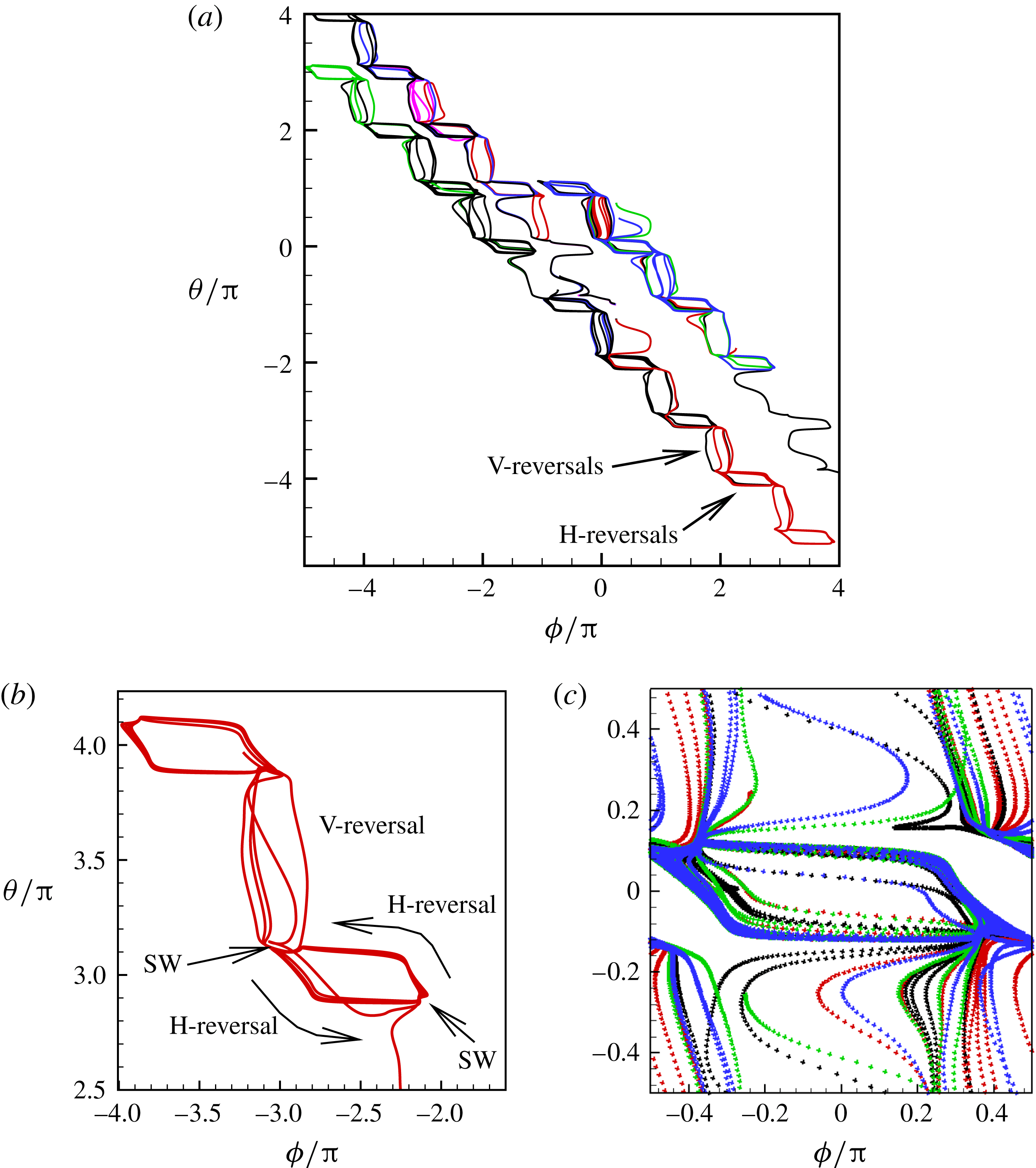
In figure 9(c), all attractors for the chaotic cases shown in figure 7 are plotted together in a periodic domain. It is observed that the trajectories are quite dense, similar to the so-called strange attractors (e.g. Lorenz). Because of the dense trajectories, the bifurcation between the V- and H-attractors occurs unpredictably, resulting in chaotic motion.
Signature of chaos in cell dynamics: (a)
 $|{\rm\Delta}\boldsymbol{X}(t)|$
(see text for definition) is plotted for several initially close trajectories; the Lyapunov exponent is obtained as the slope of the curves; (b) return map constructed from several runs; each point represents
 ${\it\theta}$
(▿) or
 ${\it\phi}$
(○) obtained at consecutive flow reversals (‘
 $n$
’ and ‘
 $n+1$
’).
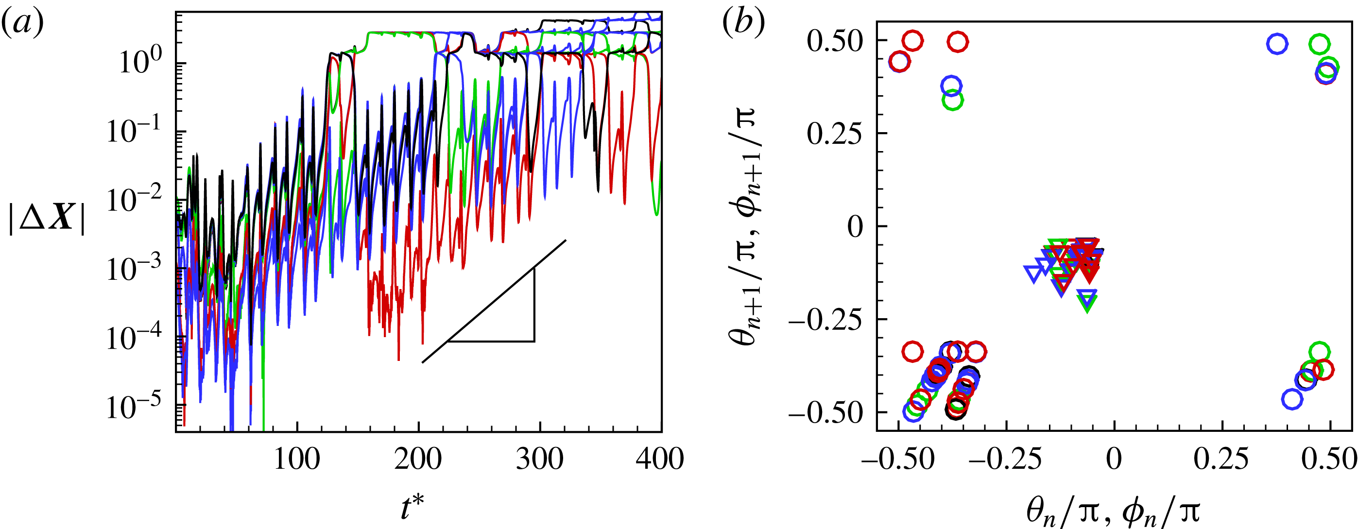
Further evidence of chaos is obtained by computing the Lyapunov exponents and a return map. A positive Lyapunov exponent indicates an exponentially diverging nature of the initially close trajectories and, hence, is a true signature of chaos. To compute the Lyapunov exponent, we assume that the cell motion is described by the angles
 ${\it\theta}$
and
 ${\it\phi}$
, and construct the vector
 ${\rm\Delta}\boldsymbol{X}(t)=\boldsymbol{X}_{i}({\it\theta},{\it\phi})-\boldsymbol{X}_{j}({\it\theta},{\it\phi})$
for two initially close trajectories. The Lyapunov exponent
 ${\it\lambda}_{i}$
is defined as
 $$\begin{eqnarray}\displaystyle |{\rm\Delta}\boldsymbol{X}(t)|=|{\rm\Delta}\boldsymbol{X}(0)|\,\text{e}^{{\it\lambda}_{i}t}. & & \displaystyle\end{eqnarray}$$
We plot
 $|{\rm\Delta}\boldsymbol{X}(t)|$
on a logarithmic scale in figure 10(a). Positive values of
 ${\it\lambda}_{i}$
in the range 0.04–0.013 are observed, further confirming the existence of chaos. In comparison, DAV reported a Lyapunov exponent of 0.013. It should be noted that a small positive value of the Lyapunov exponent is sufficient to attain diverging trajectories, and, hence, chaos. The magnitude only determines the rate of divergence. Figure 10(b) presents a return map which is constructed using the values of
 ${\it\theta}$
and
 ${\it\phi}$
obtained at two consecutive flow reversals (denoted by ‘
 $n$
’ and ‘
 $n+1$
’ in the figure). An ordered return map consisting of dense points outlining a curve is observed here, which is also an indication of chaos. In contrast, a periodic behaviour would be represented by a single pair of
 ${\it\theta}$
and
 ${\it\phi}$
, and a random process would appear as uniformly distributed points.
As an additional validation of the computational results, we have computed the Lyapunov exponent for the higher resolutions of
 $180^{3}$
and
 $240^{3}$
Eulerian grids and 49 152 Lagrangian mesh, where the exponent is computed to be 0.01–0.02, which is in agreement with the values obtained for
 $120^{3}$
and 20 480 resolutions in figure 7. As noted above, DAV reported the Lyapunov exponent 0.013, which is close to the lower bound of the range observed in our simulations.
Additionally, for the increased domain size (figure S1), the Lyapunov exponent for the chaotic dynamics is approximately 0.035, which falls in the range of values (0.013–0.04) obtained for the original domain, as noted above.
It should be noted that the chaotic dynamics is observed here at
 ${\it\lambda}$
less than physiological values.
We have performed simulations over an extended time of
 $t^{\ast }>800$
. These results are presented in the supplementary material for both the chaotic (figures S9(b) and S11) and non-chaotic cases (figures S12). The nature of the dynamics (e.g. chaotic or periodic) remains unchanged even over the longer time. The simulation time for these cases represents not only an extended dimensionless time, but also a long physical time. Our simulations show that chaos occurs even without the noise that is typically present in experiments. Chaos will continue for an infinitely long time and trajectories will continue to diverge at a rate determined by the Lyapunov exponent. As long as the Lyapunov exponent is positive, as is observed in our simulations, chaos will occur. Further, our results (e.g. figure 4
a) suggest that the initial transience from start-up could decay within a relatively short time compared with the duration of a simulation, as short as
 $t^{\ast }<30$
. It also depends on specific parameters, like
 $Ca$
,
 ${\it\lambda}$
and
 ${\it\nu}$
. The simulations presented here are performed over sufficiently long time so that the initial transience is gone. As noted above, we have extended our simulation over a long time for several representative cases, as shown in figures S9(b), S11 and S12 in the supplementary material, that clearly establish that the dynamics persists over long times.
3.2 Analysis
We now provide further analysis of the chaotic dynamics. Specifically, we address the transition between the H- and V-attractors, which is seen as a hallmark of chaos.
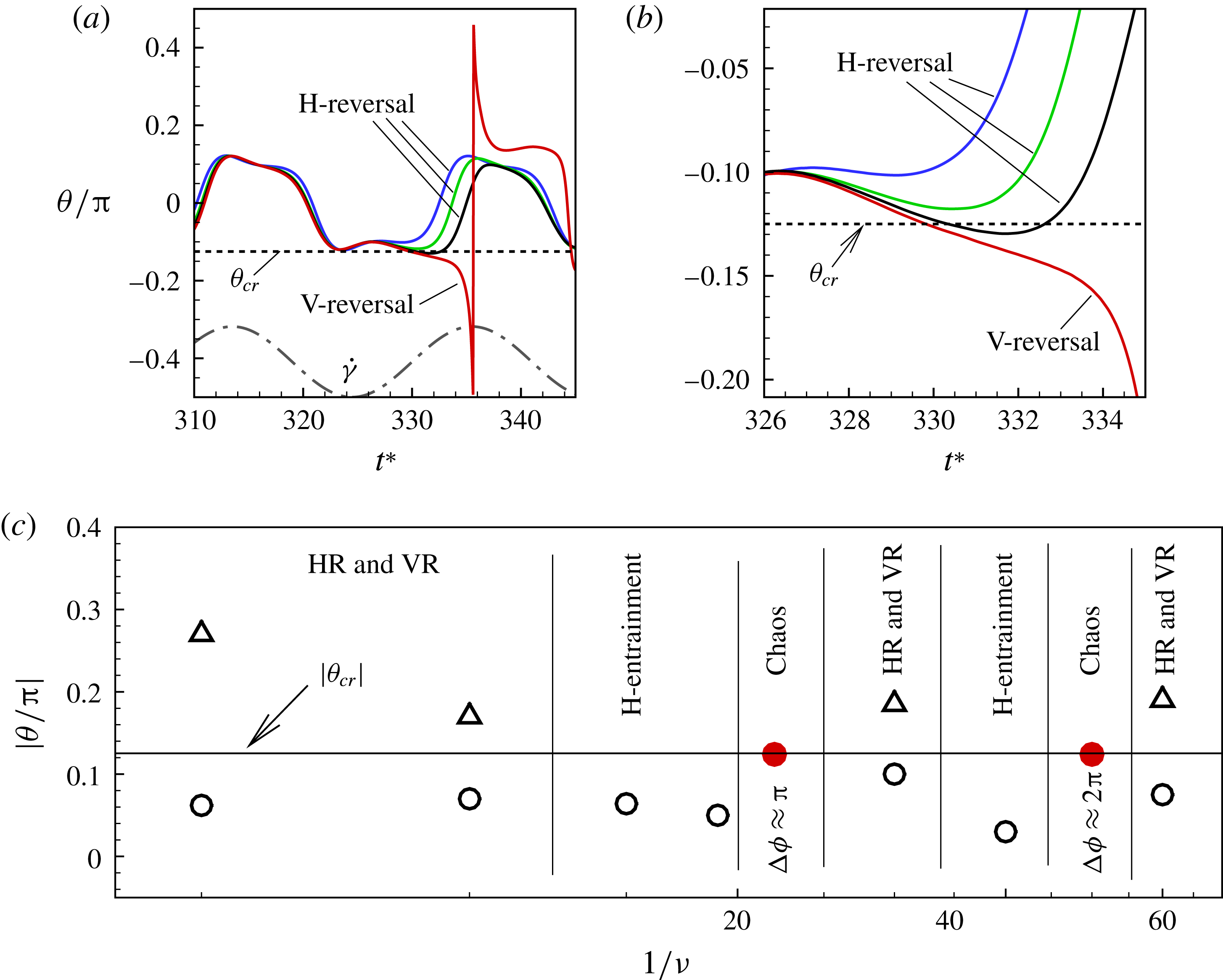
(a) Estimation of
 ${\it\theta}_{cr}$
from time series of
 ${\it\theta}$
for the chaotic cases;
 ${\it\theta}$
over a small time window is shown for a chaotic case (
 $1/{\it\nu}=22$
,
 $Ca=0.1$
,
 ${\it\lambda}=0.1$
) for four different values of
 ${\it\theta}_{o}$
. For HRs,
 ${\it\theta}_{\dot{{\it\gamma}}=0}<{\it\theta}_{cr}$
, and for VRs,
 ${\it\theta}_{\dot{{\it\gamma}}=0}>{\it\theta}_{cr}$
. (b) A close-up of (a). The flow reversal (
 $\dot{{\it\gamma}}=0$
) occurs at
 $t^{\ast }=330$
. (c) A plot of
 $|{\it\theta}_{\dot{{\it\gamma}}=0}|$
for VRs (▵), HRs (○) and chaotic dynamics (●) over a range of
 ${\it\nu}$
for fixed
 $Ca=0.1$
,
 ${\it\lambda}=0.1$
. The emergence of various dynamics with respect to varying
 ${\it\nu}$
is indicated. Here,
 ${\rm\Delta}{\it\phi}$
is the amount of membrane rotation during a half flow cycle.
Based on a posteriori analysis, we find that a VR occurs if the inclination angle
 ${\it\theta}$
at the instant of flow reversal, namely
 ${\it\theta}_{\dot{{\it\gamma}}=0}$
, exceeds a critical value
 ${\it\theta}_{cr}$
, and an HR occurs when
 ${\it\theta}_{\dot{{\it\gamma}}=0}$
is less than
 ${\it\theta}_{cr}$
. In figure 11(a,b) we plot
 ${\it\theta}$
over a small time window for a chaotic case with four different values of
 ${\it\theta}_{o}$
. It is observed that a small variation in
 ${\it\theta}$
at the instant of flow reversal can switch the limit cycle from a VR to an HR, and vice versa. One can use the time series of
 ${\it\theta}$
for the chaotic cases to obtain an estimate of
 ${\it\theta}_{cr}$
. Since for the chaotic cases the V- and H-limit cycles intersect each other,
 ${\it\theta}_{cr}$
is the maximum of
 ${\it\theta}_{\dot{{\it\gamma}}=0}$
that can be attained in an HR, or the minimum of
 ${\it\theta}_{\dot{{\it\gamma}}=0}$
that can be attained in a VR. Therefore, by careful observation through many long time series in the chaotic regime one can obtain
 ${\it\theta}_{cr}$
with a reasonable accuracy. For the cases in figure 11(a), we obtain
 ${\it\theta}_{cr}=0.124{\rm\pi}$
. As shown in figure 11(c) (by red symbols), the same value of
 ${\it\theta}_{cr}$
is obtained when the frequency is halved. For another instance of
 $Ca=0.1$
and
 ${\it\lambda}=0.3$
,
 ${\it\theta}_{cr}=0.105$
in the range
 $1/{\it\nu}=25{-}60$
. This observation suggests that
 ${\it\theta}_{cr}$
is independent of
 ${\it\nu}$
, but depends on
 $Ca$
and
 ${\it\lambda}$
.
As noted above, a VR occurs if
 ${\it\theta}_{\dot{{\it\gamma}}=0}>{\it\theta}_{cr}$
and an HR ensues if
 ${\it\theta}_{\dot{{\it\gamma}}=0}<{\it\theta}_{cr}$
. As a further illustration, we plot in figure 11(c) the values of
 ${\it\theta}_{\dot{{\it\gamma}}=0}$
for the periodic dynamics over a wide range of
 ${\it\nu}$
but fixed
 $Ca=0.1$
and
 ${\it\lambda}=0.1$
. For the periodic dynamics exhibiting two limit cycles,
 ${\it\theta}_{\dot{{\it\gamma}}=0}>{\it\theta}_{cr}$
for the VR and
 ${\it\theta}_{\dot{{\it\gamma}}=0}<{\it\theta}_{cr}$
for the HR, resulting in two non-intersecting trajectories. Therefore, a cell cannot transition between the horizontal and vertical limit cycles, and chaos is not possible in such cases. For the cases showing only the horizontal limit cycles, only one value of
 ${\it\theta}_{\dot{{\it\gamma}}=0}$
exists that is less than
 ${\it\theta}_{cr}$
.
Figure 11(c) also shows the occurrence of various dynamical regimes over a range of
 ${\it\nu}$
. It is also noted in the figure that in the chaotic regimes, the membrane displacement
 ${\rm\Delta}{\it\phi}$
in a half flow cycle occurs in integer multiples of
 ${\rm\pi}$
. Previously, in figure 9, it was noted that when the chaotic dynamics is present, one or multiple SWs occur when
 $\dot{{\it\gamma}}(t)$
is above the threshold for TB–TT transition in steady shear flow, and the bifurcation between the V- and H-limit cycles occurs via an SW. Hence, for the chaotic dynamics to appear, the cell must also swing. Since a swing is accompanied by some amount of membrane displacement, chaos cannot occur for very small values of
 $Ca$
or large values of
 ${\it\lambda}$
for which membrane displacement is suppressed. For the same reason, chaos cannot occur at a very high
 ${\it\nu}$
. It should be noted that
 ${\it\theta}_{cr}$
still exists, as shown in figure 11(c). At very high frequencies there is only a small angular oscillation of the cell axis, and thus the angle at the instant of flow reversal is very well above or below
 ${\it\theta}_{cr}$
for vertical or horizontal reversals respectively. Swinging is necessary for chaos to occur, as illustrated in figure 9(b). The frequency of cell swinging is twice the TT frequency (see, e.g. Abkarian et al.
Reference Abkarian, Faivre and Viallat2007). Thus, the flow frequency at which chaos occurs must be close to the natural TT frequency of the cell. In other words, a flow frequency close to the natural TT frequency of the cell acts as a resonator. For a full TT, the membrane displacement is 360°, i.e.
 ${\rm\Delta}{\it\phi}=2{\rm\pi}$
. For the oscillating flow, the flow direction reverses every half flow cycle. Therefore, in TT motion, the membrane rotates in one direction for every half cycle. Hence, to act as a resonator, the flow frequency should be such that the membrane rotates by an amount of
 ${\rm\pi}$
or an integer multiple of
 ${\rm\pi}$
in every half cycle. That is, the membrane displacement
 ${\rm\Delta}{\it\phi}$
, therefore, occurs in integer multiples of
 ${\rm\pi}$
. Thus, the value of
 ${\it\nu}$
at which chaos occurs is close to the TT frequency in a steady shear flow, as also predicted by the DAV model. Chaotic horizontal or vertical reversals occur about
 ${\it\theta}_{cr}$
, which is the bifurcation angle when the flow reverses. When the cell membrane rotates by nearly
 ${\rm\Delta}{\it\phi}=n{\rm\pi}$
, the membrane never comes back to exactly the same point and therefore the swinging angle at the instant of flow reversal is never quite the same, although it is always close to the critical angle. As a result, the RBC cannot synchronize with the flow and therefore irregular reversals occur, and with each flow cycle the location of a point in
 ${\it\theta}$
–
 ${\it\phi}$
phase space at the same shear rate is never the same. Therefore, the instantaneous
 ${\it\theta}(t)$
is sometimes above
 ${\it\theta}_{cr}$
and sometimes below, but not in any regular sequence, leading to the bifurcation. In simple terms, the flow frequency must be such as to allow for the membrane to traverse from one side of the cell to the other (half a TT cycle) before the flow reverses for chaos to occur. Thus, chaos occurs when the forcing frequency of the flow is close to the natural TT frequency of the RBC, which also causes
 ${\rm\Delta}{\it\phi}\approx n{\rm\pi}$
.
When the membrane is not able to make an
 $n{\rm\pi}$
rotation in a half flow cycle, periodic dynamics in the form of HR and VR or only HR occur. For example,
 ${\rm\Delta}{\it\phi}\approx 1.7{\rm\pi}$
in figure 5(a,b), where only HR is observed.
It may be noted that in order to calculate
 ${\it\theta}_{cr}$
, one has to consider the chaotic trajectories as described above. However, once the value of
 ${\it\theta}_{cr}$
for a specific
 $Ca$
and
 ${\it\lambda}$
is found, it is applicable to other frequency ranges.
Analysis of H-entrainment for the cases shown in figure 5(a). Here, (a,b) show the locations of the same marker point on the cell membrane at an early time
 $t^{\ast }=10$
and at a later time
 $t^{\ast }=120$
respectively, for different initial orientations
 ${\it\theta}_{o}$
as indicated; (c) shows a time sequence of contour-averaged membrane strain energy for
 ${\it\theta}_{o}=0$
(black),
 ${\rm\pi}/4$
(red),
 ${\rm\pi}/2$
(blue),
 $-{\rm\pi}/4$
(green).

Some insights can be obtained by considering the strain energy variation of the cell membrane over time. For this, we consider the entraining trajectories shown previously in figure 5(a), where the cells started with different
 ${\it\theta}_{o}$
exhibit different dynamics during the early time, but settle about the same horizontal limit cycle over a long time. To elucidate the entrainment process, the locations of the same marker point on the membrane are shown in figures 12(a) and 12(b) at an early time and a later time respectively for different values of
 ${\it\theta}_{o}$
. At the early time, the same marker point ends up in different
 ${\it\phi}$
locations for different
 ${\it\theta}_{o}$
. At the later time, the marker points for all values of
 ${\it\theta}_{o}$
are located at the same
 ${\it\phi}$
. This observation implies a reorganization of the membrane over time in which a net membrane displacement occurs in each flow cycle, but the amount of displacement is dependent on
 ${\it\theta}_{o}$
. A redistribution of the membrane strain energy also occurs, as shown in figure 12(c), where the strain energy
 $W$
averaged over the cell contour is plotted for various values of
 ${\it\theta}_{o}$
. During the early time, cells with different values of
 ${\it\theta}_{o}$
have different waveforms of
 $W$
, but at later times, all
 $W$
curves merge, and the cells are locked into one stable attractor.
For the VR and HR also, the strain energy is observed to attain symmetric waveforms with respect to the flow cycle, although the nature of the waveforms in the two cases is different. In contrast, for the chaotic dynamics, the waveform is aperiodic.
Unlike a rigid ellipsoid in the absence of inertia, a deformable cell lags in its response to flow variation. We define the phase lag between the flow and the cell inclination as
 ${\it\Phi}=2{\rm\pi}\tilde{{\it\nu}}(t_{\dot{{\it\gamma}}_{a}}-t_{{\it\theta}=0})$
, where
 $t_{\dot{{\it\gamma}}_{a}}$
and
 $t_{{\it\theta}=0}$
are respectively the time instances when
 $\dot{{\it\gamma}}=\dot{{\it\gamma}}_{a}$
and when
 ${\it\theta}=0$
. Figure 13 shows that
 ${\it\Phi}$
generally decreases with decreasing
 ${\it\nu}$
, but non-monotonically with a sawtooth pattern. A monotonic decrease occurs in the frequency ranges where periodic dynamics is observed. As noted previously in figure 11(c), the chaotic regimes appear in the frequency space between the regimes of periodic dynamics. The decreasing trend of
 ${\it\Phi}$
occurs until a chaotic regime is encountered. Within a chaotic regime,
 ${\it\Phi}$
does not show any consistent trend as the cells cannot synchronize with the flow. As
 ${\it\nu}$
is further decreased so that the RBC exits the chaotic regime to assume a periodic dynamics, a decreasing trend is re-established, followed by a jump in
 ${\it\Phi}$
. The computed trend of
 ${\it\Phi}$
is compared with the DAV model in figure 13, which shows a good agreement between the two.
Effect of
 ${\it\nu}$
on phase lag
 ${\it\Phi}$
: simulation results (—▫—) and DAV model (- - ▵ - -). Here,
 ${\it\lambda}=1$
,
 $Ca=0.1$
.

3.3 Effect of
 ${\it\lambda}$

We now vary both
 ${\it\lambda}$
and
 ${\it\nu}$
but keep
 $Ca$
fixed at 0.1. The cell dynamics can be best described using a
 ${\it\lambda}$
–
 ${\it\nu}$
phase plot, as shown in figure 14. Different dynamics as already described in the previous sections also appear as
 ${\it\lambda}$
is varied. Namely, we observe dynamics with two limit cycles characterized by periodic VRs and HRs, a single limit cycle characterized by H-entrainment, multiple limit cycles representing non-coalescing HRs and chaotic dynamics. Different regimes appear as banded regions in the
 ${\it\lambda}$
–
 ${\it\nu}$
space. Chaotic regimes occur between regions of periodic dynamics. As
 ${\it\lambda}$
is increased, chaotic regimes occur at reduced
 ${\it\nu}$
, as a result of the slower membrane movement. In addition, at higher
 ${\it\lambda}$
near physiological values, chaos is no longer observed as membrane rotation is suppressed; instead, a rigid-body-like oscillation is observed.
We also compare our simulation with the phase diagram obtained by the DAV model in figure 14. Both the simulation and the DAV model predict very similar regimes in phase space at small deformation of the cell, as seen in the figure which is for
 $Ca=0.1$
. Some minor differences may be noted; e.g. the non-coalescing HR dynamics is not predicted by the DAV model. Moreover, the chaotic regimes persist at higher
 ${\it\lambda}$
in the DAV model than in the simulations.
Effect of
 ${\it\lambda}$
. Different dynamics are shown in a
 ${\it\lambda}$
–
 ${\it\nu}$
phase plot. (a) Simulation results; (b) DAV model. Chaotic dynamics (▾); periodic dynamics: HR and VR (▪), H-entrainment (●), non-coalescing HR (▴), rigid-body-like oscillations (♢). Here,
 $Ca=0.1$
.

Suppression of chaos at higher
 ${\it\lambda}$
can also be understood in terms of the critical inclination
 ${\it\theta}_{cr}$
. Figure 15(a) shows that
 ${\it\theta}_{cr}$
decreases with increasing
 ${\it\lambda}$
. As a result, the RBC is unable to hop between V- and H-limit cycles, thereby reducing the possibility of chaos.
The oscillation amplitude
 ${\rm\Delta}{\it\theta}$
is also observed to decrease with increasing
 ${\it\lambda}$
, as shown in figure 15(b), as long as
 ${\it\lambda}$
is approximately less than the threshold value for the TB–TT transition in steady shear flows. For
 ${\it\lambda}$
above the threshold,
 ${\rm\Delta}{\it\theta}$
tends to increase abruptly with increasing
 ${\it\lambda}$
as the rigid-body-like oscillation ensues.
The effect of
 ${\it\lambda}$
on the phase lag
 ${\it\Phi}$
is shown in figure 15(c). In general, a decrease in
 ${\it\Phi}$
is observed with increasing
 ${\it\lambda}$
. At high
 ${\it\lambda}$
, the phase lag approaches zero as the cell dynamics approaches that of a rigid body. For
 ${\it\lambda}\lesssim 1$
and for some
 ${\it\nu}$
, a sawtooth-like trend is observed because of the appearance of the chaotic regimes between the regimes of periodic motion in the phase space.
Both
 ${\rm\Delta}{\it\theta}$
and
 ${\it\Phi}$
predicted by the DAV model show similar qualitative trends to those in the simulations. This is shown in figure 15(b,c), where results from the DAV model are shown along with our simulation results.
(a) Effect of
 ${\it\lambda}$
on
 ${\it\theta}_{cr}$
: ● represents
 ${\it\theta}_{cr}$
, ▫ represents
 ${\it\theta}_{\dot{{\it\gamma}}=0}$
for HR and ▵ represents
 ${\it\theta}_{\dot{{\it\gamma}}=0}$
for VR. (b,c) Effect of
 ${\it\lambda}$
on the oscillation amplitude
 ${\rm\Delta}{\it\theta}$
and phase lag
 ${\it\Phi}$
. The continuous red lines with filled symbols are the simulation results. The dotted black lines with unfilled symbols are the DAV model:
 $1/{\it\nu}=15$
(▫), 30 (▵), 50 (▿).

3.4 Effect of
$Ca$

The effect of
 $Ca$
is shown in figure 16 using a
 $Ca$
–
 $1/{\it\nu}$
phase-space plot. As before, the dynamical regimes observed are HR and VR characterized by two stable limit cycles, H-entrainment with a single limit cycle, non-converging HR resulting in multiple limit cycles and chaos. It should be noted that ‘non-converging’ trajectories are indeed periodic, unlike the chaotic cases. However, they are ‘non-converging’ because cells with different initial conditions do not merge in to identical trajectories, although they exhibit periodicity. At a very low
 $Ca$
, a rigid-body-like oscillation is observed at reduced
 ${\it\nu}$
. As
 ${\it\nu}$
is increased and
 $Ca$
is held constant, regimes with H-entrainment followed by HR and VR appear. At this low
 $Ca$
, no chaotic dynamics is observed since the membrane rotation is suppressed. As
 $Ca$
is increased to allow some amount of membrane rotation, regions with the chaotic dynamics appear which are preceded and followed by regions of H-entrainment. Qualitative similarity between the simulation results and the DAV model is also noticed at smaller values of
 $Ca$
. However, at higher
 $Ca$
, there is a disagreement between the two. Whereas the DAV model predicts a persistence of the chaotic dynamics at high shear rate, and even a broadening of the chaotic region, the simulation results suggest that the chaotic regions narrow and become fully suppressed at
 $Ca\gtrsim 0.5$
. The difference arises, as is evident, due to the assumption of a fixed shape of the cells in the DAV model. Hence, cell deformation suppresses the chaotic behaviour at large shear rates.
The effect of
 $Ca$
is shown by
 $Ca$
–
 $1/{\it\nu}$
phase plots. (a) Simulation; (b) DAV model; ▫, VR and HR; ○, H-entrainment; ▿, chaos;
 ${\rm\Delta}$
, non-converging HR; ♢, rigid-body-like oscillation. (c) Sequence of cell deformation for
 $Ca=0.5$
,
 $1/{\it\nu}=44$
. In the upper row, the cell axis moves from the first to the second quadrant. The reverse motion is shown in the lower row. For all data,
 ${\it\lambda}=1$
.
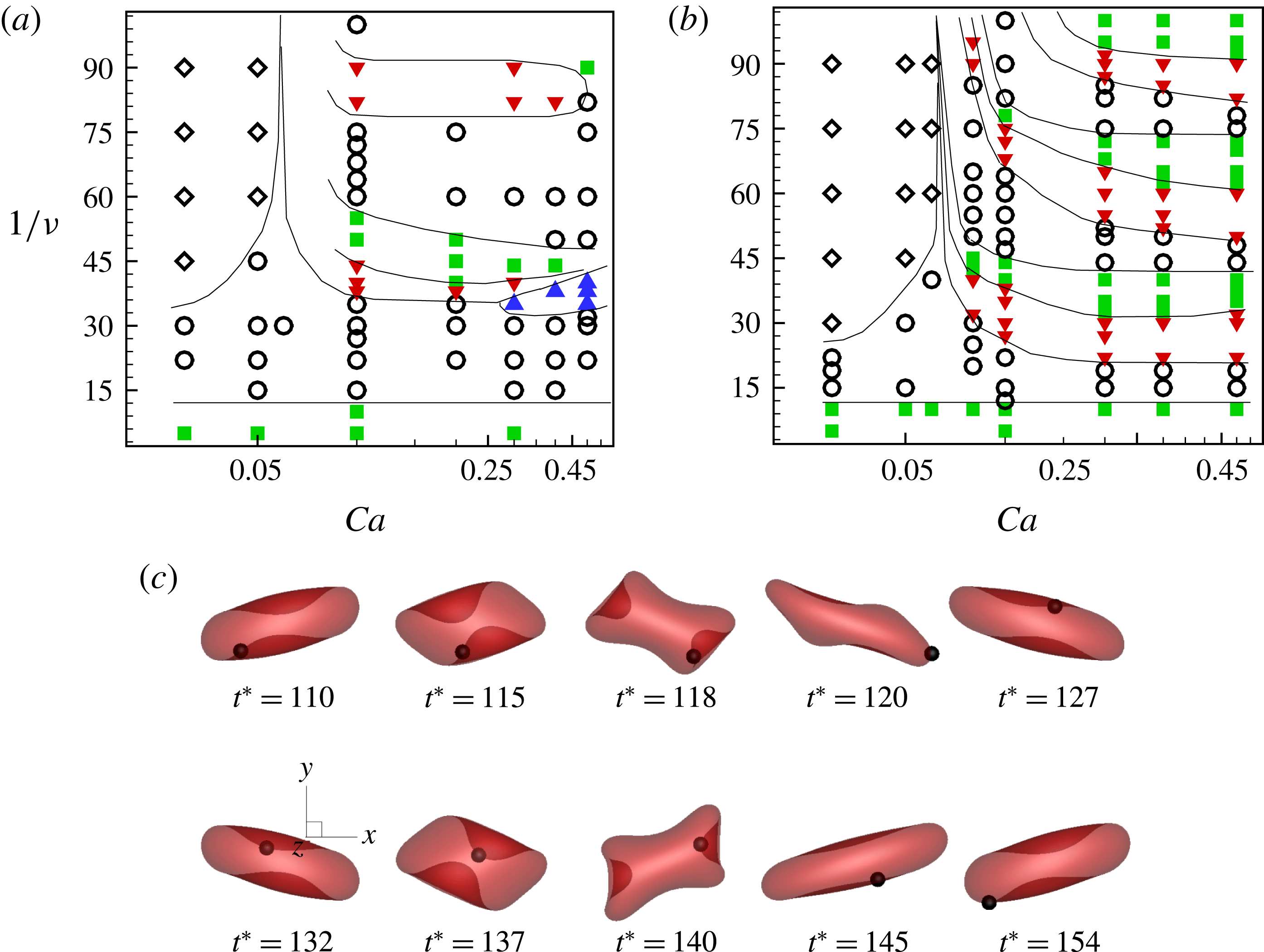
Due to the large deformation at high
 $Ca$
, it is sometimes difficult to establish whether a cell is undergoing a VR or an HR. In fact it appears that at high
 $Ca$
, the cell reversals are driven by deformation, as shown in figure 16(c). Here, the cell gets elongated along the first quadrant near the peak shear. There is a phase lag between the cell and the flow reversal. As the flow reverses, the extensional and compressional directions are interchanged, and the cell is compressed along the rim and elongated along the dimple. As the reverse flow is fully established, the cell elongates completely in the second quadrant. Often, an asymmetry in cell deformation between successive reversals is observed which is a result of different portions of the strain energy barrier encountered by the membrane during the first and second halves of a flow cycle. This behaviour contrasts with the redistribution of the phase of membrane rotation to a symmetric one, which was noted earlier for the H-entrainment occurring at low to moderate
 $Ca$
. At higher
 $Ca$
,
 ${\it\theta}$
and
 ${\it\phi}$
often do not fully entrain, and the effect of the initial conditions is preserved even after a long time, resulting in the non-converging trajectories.
Effect of
 $Ca$
. (a–c) Time series of
 ${\it\theta}$
and
 ${\it\theta}$
–
 ${\it\phi}$
phase plot for
 $1/{\it\nu}=30$
, 60, 75 respectively;
 $Ca=0.03$
(black thin continuous line), 0.05 (black thick dashed line), 0.1 (blue dash-dot line), 0.2 (green dashed line), 0.5 (red continuous line). (d) Amplitude of angular oscillation
 ${\rm\Delta}{\it\theta}$
for various values of
 $Ca$
. (e) Phase lag
 ${\it\Phi}$
as a function of
 $Ca$
.
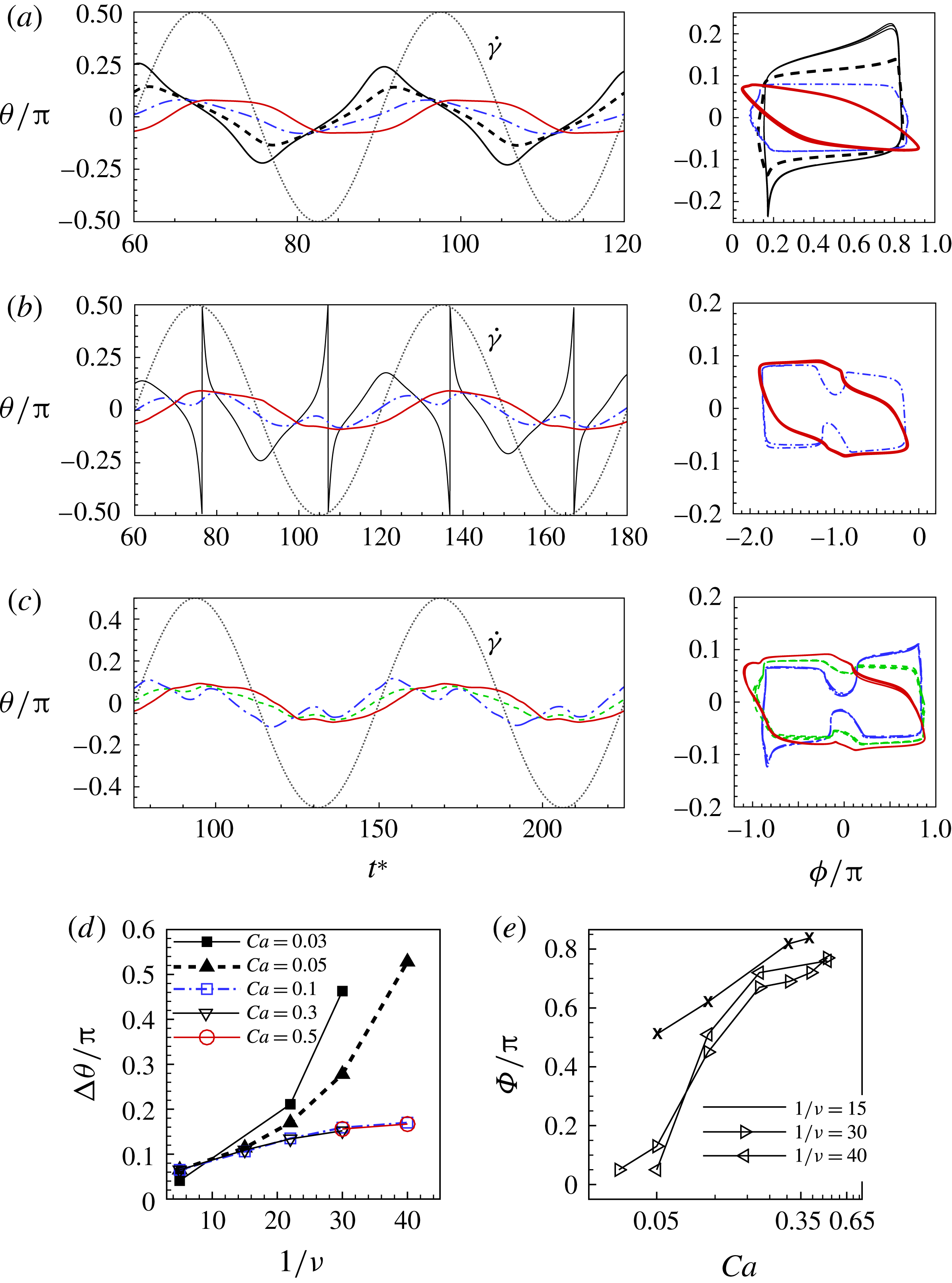
The effect of
 $Ca$
on
 ${\it\theta}(t)$
is shown in figure 17(a–c). At moderate dimensionless frequency (
 $1/{\it\nu}=30$
in the figure), increasing
 $Ca$
results in a greater phase lag while reducing the amplitude of oscillation. At a small
 $Ca$
, the phase lag is nearly zero as the RBC exhibits a rigid-body-like motion. As
 $Ca$
is increased, the phase lag is also observed to increase due to a greater amount of membrane rotation. Moreover, the
 ${\it\theta}(t)$
waveform changes from a peaked shape to a more flattened curve as the RBC performs a partial swinging. At reduced frequencies (
 $1/{\it\nu}=60$
and 75 in the figure), the cell has more time to respond before the flow reverses. At a small
 $Ca$
it can sweep a large angle resembling a partial TB. At moderate
 $Ca$
, SW occurs as
 $\dot{{\it\gamma}}$
approaches its peak, and an inflection is observed in the
 ${\it\theta}$
–
 ${\it\phi}$
phase plot. At even higher
 $Ca$
, SW is suppressed and the inflection in the
 ${\it\theta}$
–
 ${\it\phi}$
curve vanishes. Figure 17(d,e) shows the
 $Ca$
effect on the oscillation amplitude
 ${\rm\Delta}{\it\theta}$
and the phase lag
 ${\it\Phi}$
. At small
 $Ca$
,
 ${\rm\Delta}{\it\theta}$
increases with decreasing
 ${\it\nu}$
following a rigid-body-like motion. At higher
 $Ca$
,
 ${\rm\Delta}{\it\theta}$
initially increases with decreasing
 ${\it\nu}$
but then reaches a saturation since the maximum inclination that a cell can attain is limited by the steady flow results. The phase lag increases with increasing
 $Ca$
, as the cell reversals become increasingly driven by deformation.
Cell deformation in the shear plane. (a,b) Time sequence of
 $D_{12}$
,
 $L$
and
 $B$
at
 $Ca=0.5$
,
 ${\it\lambda}=1$
in a steady shear flow (thick black line) and in oscillating shear flows at
 $1/{\it\nu}=30$
(dashed red line) and 60 (thin blue line). (c–e) The cell shapes at steady shear flow, and at oscillating shear flows at
 $1/{\it\nu}=30$
and 60 respectively.

3.5 Deformation
As noted above, at higher shear rates, a significant amount of deformation occurs as the cell reverses its orientation in response to the flow reversals. To quantify the cell deformation in the shear plane, we consider a quantity similar to the Taylor deformation parameter, defined as
 $D_{12}=(L-B)/(L+B)$
, where
 $L$
and
 $B$
are the maximum and minimum distance of the cell surface from the centroid in the shear plane. We note that
 $L$
and
 $B$
may not be perpendicular to each other as the cell assumes a complex shape, as in figure 16(c). Figure 18(a) compares the time series of
 $D_{12}$
in steady and oscillatory shear flows (
 $1/{\it\nu}=30$
and 60) for
 $Ca=0.5$
. In the steady shear flow,
 $D_{12}$
shows a small oscillation which arises due to the swinging motion of the cell. In contrast, a significantly larger oscillation is observed in the oscillating shear flow which is due to the orientation reversals of the cell. Most strikingly,
 $D_{12}$
in oscillating flows exhibits large overshoots and/or undershoots compared with that in a steady flow. Instantaneous cell shapes are shown in figure 18(c) for a steady shear flow and in figure 18(d,e) for oscillating flows. Significantly more deformed shapes are observed in the latter cases. In particular, the cell can take on very complex shapes during the orientation reversals, resulting in the overshoots and undershoots in
 $D_{12}$
. Instantaneous
 $L$
and
 $B$
are plotted in figure 18(b), which shows that
 $L$
and
 $B$
in the oscillating flows are generally lower than those in the steady flow. The result implies that the cell elongation in an oscillating flow is less but the cell compression is higher than their counterparts in the steady flow. An overshoot in
 $D_{12}$
occurs when both
 $L$
and
 $B$
reach their minima; at this instance, the cell shape becomes compressed but remains biconcave, e.g. at
 $t^{\ast }=63$
in figure 18(d). For some
 ${\it\nu}$
, e.g.
 $1/{\it\nu}=30$
in the figure, instantaneous
 $B$
could be higher than that in the steady flow and shows a cusp-like jump. Consequently, an undershoot in
 $D_{12}$
occurs. This happens when the cell assumes a quad-concave shape during flow reversals, thereby significantly deviating from the biconcave shape, e.g. at
 $t^{\ast }=66$
in figure 18(d).
(a) Time series of
 $D_{12}$
at
 $Ca=0.3$
,
 ${\it\lambda}=1$
in a steady shear flow (thick black line) and in oscillating shear flows at
 $1/{\it\nu}=35$
(thin black line), 40 (dash-dot red line) and 44 (dashed green line), corresponding to H-entrainment, chaotic dynamics and VR respectively. (b) Cell shapes for the chaotic case at
 $1/{\it\nu}=40$
near a reversal;
 $t^{\ast }=84$
and 88 respectively correspond to an overshoot and an undershoot in
 $D_{12}$
.

We find that undershoots in
 $D_{12}$
occur more frequently during VRs than HRs. This is illustrated in figure 19, where
 $D_{12}$
is shown for
 $1/{\it\nu}=35$
, 40 and 44, which correspond to H-entraining, chaos and VR respectively. For
 $1/{\it\nu}=35$
, only overshoots are observed, while for
 $1/{\it\nu}=40$
and 44, both overshoots and undershoots are observed. The cell shapes are shown in figure 19(b) for the chaotic case near an instance of a reversal. They further support the previous observation that an overshoot occurs when the cell shape becomes compressed but remains biconcave (e.g. at
 $t^{\ast }=84$
), and an undershoot occurs when the cell assumes a quad-concave shape, thereby significantly deviating from the biconcave shape (e.g. at
 $t^{\ast }=88$
).
Cell deformation in an off-shear plane. (a) Time sequence of
 $D_{13}$
at
 $Ca=0.1$
,
 ${\it\lambda}=0.1$
in a steady shear flow (thick black line) and in oscillating shear flow at
 $1/{\it\nu}=60$
for HR (dashed blue line) and VR (dash-dot red line). (b) A phase-space plot of
 $D_{13}$
–
 ${\it\theta}$
for the cases shown in (a). (c) Phase-space plot for the chaotic dynamics at
 $Ca=0.1$
,
 ${\it\lambda}=0.1$
,
 $1/{\it\nu}=25$
. The result for steady flow is shown by the thick black line.

In several prior studies (e.g. Watanabe et al.
Reference Watanabe, Kataoka, Yasuda and Takatani2006; Noguchi Reference Noguchi2010), cell deformation was reported using an off-shear plane deformation parameter
 $D_{13}=(L-Z)/(L+Z)$
, where
 $Z$
is the maximum distance of the cell surface from the centroid in the direction perpendicular to the shear plane. Figure 20(a) shows the time series of
 $D_{13}$
in steady and oscillating shear flows. In the steady flow,
 $D_{13}$
oscillates due to cell swinging. A larger variation occurs in oscillating flows due to the increased cell deformation. Strikingly,
 $D_{13}$
is positive in the steady flow, but it can assume negative values in the oscillating flows. The negative
 $D_{13}$
occurs when the cell reverses its orientation, and is due to the greater amount of compression, which also results in large undershoots, particularly during a VR. It should be noted that for the relatively low
 ${\it\nu}$
chosen in this figure (
 $1/{\it\nu}=60$
), the cell executes a swing near the peak
 $\dot{{\it\gamma}}$
. Consequently,
 $D_{13}$
in steady flow nearly overlaps with that in oscillating flow at peak shear for V- and H-reversals with a phase offset.
Figure 20(b) shows a phase-space plot of
 $D_{13}$
versus
 ${\it\theta}$
for the periodic dynamics. It shows that a greater amount of variation in
 $D_{13}$
occurs in a VR as the cell sweeps a wider angle. There is an overlap in the deformation phase plot between the HR, the VR and the steady flow, as illustrated by the oblong loops occurring near the maximum
 $D_{13}$
. The looping structure is indicative of swinging and is illustrative of the deformation dependence of the cell on the instantaneous orientation and phase of membrane rotation. Such a complex looping component has not been reported previously.
Figure 20(c) shows a phase-space plot for a set of chaotic dynamics. An interesting butterfly-shaped pattern is observed here which comprises dense but non-overlapping trajectories arising due to a lack of synchronization between the cell and the imposed shear.
Figure 21 shows the amplitude of
 $D_{13}$
, defined as
 ${\rm\Delta}D_{13}=\max \{D_{13}\}-\min \{D_{13}\}$
, and the time average deformation
 $\langle D_{13}\rangle$
as functions of
 $Ca$
for different frequencies. Also plotted is the result for the steady flow at the same
 $Ca$
. In general,
 ${\rm\Delta}D_{13}$
increases with increasing
 $Ca$
and decreasing
 ${\it\nu}$
. It is also evident from the figure that
 ${\rm\Delta}D_{13}$
is higher in a VR than in an HR due to a higher sweep angle, as already noted before. Further, except at a high
 ${\it\nu}$
,
 ${\rm\Delta}D_{13}$
is higher than those in steady flows. At high frequencies,
 ${\rm\Delta}D_{13}$
is lower than in steady shear because
 $D_{13}$
is limited by the fast flow reversal and the cell does not have enough time to fully deform.
The average deformation
 $\langle D_{13}\rangle$
is always higher in steady shear since the cell is always in the extensional quadrant and it undergoes much less compression compared with that in oscillating shear. Moreover,
 $\langle D_{13}\rangle$
for an HR is higher than that for a VR, since instantaneous
 $D_{13}$
can be negative for the latter case. As expected,
 $\langle D_{13}\rangle$
increases with decreasing
 ${\it\nu}$
. Interestingly, however, a non-monotonic trend is observed with respect to
 $Ca$
at moderate to high frequencies:
 $\langle D_{13}\rangle$
first increases but then decreases with increasing
 $Ca$
. The origin of this trend is again the large compression of the cell that occurs during flow reversals. At moderate to high frequencies, the cell spends a significant fraction of a flow cycle in this compressed state which becomes more severe as
 $Ca$
is increased, resulting in a decrease in the average deformation. However, at low frequencies, the cell spends significantly more time in the TT/SW mode in the extensional quadrant before reversing its direction and thus resulting in a monotonic increase in
 $\langle D_{13}\rangle$
with increasing
 $Ca$
.
Dependence of (a)
 ${\rm\Delta}D_{13}$
and (b)
 $\langle D_{13}\rangle$
on
 $Ca$
for various frequencies as
 $1/{\it\nu}=5$
(▫), 22 (▵), 30 (
 $\times$
), 44 (♢), 50 (○), 60 (▿), 75 (▹). Solid lines represent HR and dashed lines VR. The result for the steady shear flow is shown by the thick black line.

3.6 Off-shear plane drift
In all of our simulations, only the initial (at
 $t^{\ast }=0$
) orientation of the axis of revolution of the cell is aligned along the shear plane. No restriction is imposed on the orientation as the simulation evolves in time. Since the simulations are fully three-dimensional, the axis may drift out of the shear plane depending on the specific parameters chosen. For the most part of the parameter space that is considered here, the cell axis naturally remains aligned in the shear plane. Figure 22 shows two sample cases: a chaotic dynamics case and a rigid-body-like oscillation case. For the chaotic dynamics, the cell axis naturally remains aligned in the shear plane without any significant drift, as seen in the figure. For the rigid-body-type oscillation, which occurs at very small values of
 $Ca$
or very large
 ${\it\lambda}$
, there is a significant off-plane drift. It was shown in our previous works, namely Cordasco & Bagchi (Reference Cordasco and Bagchi2013) and Cordasco et al. (Reference Cordasco, Yazdani and Bagchi2014), that the off-plane drift is suppressed if some amount of membrane displacement is allowed. In contrast, a significant drift occurs when the membrane rotation is suppressed. As proven in the previous sections, all of the interesting dynamics presented here, namely the chaotic dynamics, HR, VR and entrainment, require a significant amount of membrane displacement. Consequently, the off-plane drift is suppressed for most of the cases presented here.
Furthermore, in Cordasco & Bagchi (Reference Cordasco and Bagchi2013), the stress-free state of the cell was taken to be the natural biconcave shape. Later, in Cordasco et al. (Reference Cordasco, Yazdani and Bagchi2014), we compared the dynamics of the cell under two different stress-free states – a nearly spherical shape as in the present work and the natural biconcave shape as in Cordasco & Bagchi (Reference Cordasco and Bagchi2013). We showed that the nearly spherical shape of the stress-free state retains the TT motion over a larger parameter space than the biconcave stress-free state. This is consistent with the experimental observation of Dupire et al. (Reference Dupire, Socol and Viallat2012). Cordasco et al. (Reference Cordasco, Yazdani and Bagchi2014) presented a phase diagram that showed that the cell with the nearly spherical stress-free state performs TT motion with its axis aligned in the shear plane at shear rates well below
 $Ca\sim 0.1$
, at which the cell with the biconcave stress-free state would tumble. Hence, the present results are consistent with our previous study provided that the quasi-spherical stress-free state is considered.
The off-shear plane drift is shown using the tilt angle
 ${\it\psi}$
for two sample runs: for a cell at low
 $Ca$
exhibiting a rigid-body-like oscillation (solid red line,
 $Ca=0.05$
) and the chaotic dynamics (dashed blue line,
 $Ca=0.1$
). The tilt angle is defined as
 ${\it\psi}=\tan ^{-1}(z/\sqrt{x^{2}+y^{2}})$
, where
 $x,y,z$
are the coordinates of a point on the axis of revolution of the RBC. The cell exhibits a significant off-plane drift for the rigid-body-like motion, but stays aligned in the shear plane for the chaotic motion.

3.7 Influence of reduced volume and stress-free state
In order to assess the contribution of the reduced volume to the onset of the chaotic dynamics, we have performed an extensive number of simulations using oblate capsules of reduced volumes 0.997–0.644; the last value corresponds to the reduced volume of the RBC. The initial shape is taken to be the stress-free state. Some of these results are given in the supplementary material in figures S2–S6, and S13, S14, and table 1 there. The major conclusions from the oblate capsule simulations are as follows. Chaotic dynamics is not observed for oblate capsules for reduced volumes as low as 0.766. Specifically, for reduced volumes 0.997–0.965, only periodic dynamics in terms of horizontal and vertical reversals is observed (figures S3 and S4). Similar entrainment dynamics is also observed for the oblate capsules (figure S2). For reduced volumes 0.872–0.766, a unidirectional flipping motion is also observed in addition to periodic dynamics (figure S5). When the reduced volume is close to that of the RBC (i.e. 0.644), an irregular sequence of swinging and tumbling occurs which is indicative of the onset of chaos (figure S13). Thus, chaos occurs for oblate capsules as the reduced volume approaches that of the RBC.
The amount of membrane rotation
 ${\rm\Delta}{\it\phi}$
over one half period of the imposed flow as a function of the reduced volume is presented in table 1 in the supplementary material. The results suggest that for larger reduced volume,
 ${\rm\Delta}{\it\phi}$
is much larger than
 $n{\rm\pi}$
, and as the reduced volume approaches that of the RBC,
 ${\rm\Delta}{\it\phi}$
approaches
 $n{\rm\pi}$
. It should, however, be noted that a membrane rotation of
 $n{\rm\pi}$
is not a sufficient condition for chaos to occur. As shown above, chaos occurs in narrow bands in parameter space, and only when several conditions are met. The cell must be swinging, and must not deform significantly. Further, the swinging must occur near the instant of flow reversal.
It should also be noted that as the reduced volume of the oblate approaches that of the RBC, the shape no longer remains an oblate. Instead, the shape naturally transitions to biconcave due to the presence of the membrane bending. This is shown in figure S14. Thus, at these reduced volumes, it is sufficient just to consider the RBC rather than the oblate.
We have also performed additional simulations with initially spherical capsules under varying surface area dilation. For an extensible surface, we take the area dilation parameter
 $C=1$
. For a nearly inextensible surface, we take
 $C=1000Ca$
, as already discussed in § 2. One sample result is given in figure S6 in the supplementary material. Additional analysis of the initially spherical capsules can be found in Zhao & Bagchi (Reference Zhao and Bagchi2011). The initially spherical capsules show only symmetric oscillations in response to the altering flow directions. No chaotic dynamics is observed for the initially spherical capsules either. For the initially spherical capsules, no chaotic dynamics is possible as there is no swinging dynamics for such capsules in a steady shear flow. As noted in §§ 3.1.2 and 3.2, the swinging dynamics is necessary for chaos to occur as it acts as a bifurcation between HR and VR.
In order to assess the influence of the asphericity of the stress-free shape, we performed additional simulations in which the biconcave resting shape was taken as the stress-free state. We refer to this configuration as biconcave stress-free (BCSF,
 $V_{0}=0.644$
) as opposed to the nearly spherical stress-free state (SSF,
 $V_{0}=0.997$
) used so far. These results are presented in the supplementary material (figures S7–S9). Interestingly, we find the same behaviour for the BCSF case, namely the regular HR, VR, H-entrainment and the chaotic dynamics. Hence, the stress-free state (BCSF or SSF) does not qualitatively alter the observed dynamics. Moreover, the reduced volume determines whether chaotic dynamics can be present or not.
4 Conclusion
A 3D computational study on the dynamics of fully deformable RBCs in oscillatory shear flow has been presented. Simulations performed over a wide range of dimensionless frequency, viscosity ratio and shear rate amplitude show that the RBC reverses its orientation in response to the alternating flow direction by passing through either the flow axis resulting in horizontal cell reversals or the flow gradient axis resulting in vertical reversals. The dynamics are often periodic and, hence, the cell settles into a periodic sequence of either horizontal or vertical reversals depending on the initial orientation. In many cases, the initial conditions are completely forgotten and the cells become entrained in the same sequence of horizontal reversals. Additionally, within a certain parameter range, small differences in the initial orientations can result in periodic yet distinct horizontal reversals. For low forcing frequencies, the cell dynamics appears as a combination of horizontal or vertical reversals near the instant of flow reversals along with one or multiple swings near the maximum shear rate. Different dynamical regimes observed in our simulations are schematically presented in figure 23. The peak shear rate and dimensional frequency considered here are approximately in the ranges of 0.3–
 $300~\text{s}^{-1}$
and 0.0025–60 Hz respectively. This falls within the physiological range, as a nominal human heart rate is 1 Hz and the vasculature can fluctuate at higher or lower frequency.
The major dynamical regimes of RBC motion observed.

Chaotic dynamics, as previously observed in experiments and predicted by reduced-order models, is also observed in our simulations. The present study is the first to conclusively show the chaotic dynamics of RBCs in oscillatory shear flow. Such dynamics is characterized by a non-periodic sequence of swings, and horizontal and vertical reversals, and is obtained in our study with a fully deterministic numerical model without the introduction of any stochastic noise such as thermal fluctuations. The chaotic dynamics, however, occurs at a viscosity ratio less than the physiological value. We further present strong evidence that such dynamics is chaotic in nature by calculating the positive Lyapunov exponents which illustrate the divergent trajectories of RBCs with initially very close orientations over long times.
We provide a detailed analysis of the chaotic dynamics of the RBC. In the chaotic regime, while the sequence of the horizontal and vertical reversals remains unpredictable, we have presented a novel finding that the occurrence of a vertical or horizontal reversal depends only on whether a critical angle is exceeded at the instant of flow reversal. Remarkably, the chaotic trajectories consistently show a bifurcation about this angle. We found that the critical angle is independent of
 ${\it\nu}$
. We emphasize that the emergence of the chaotic behaviour is coupled to the occurrence of the swinging dynamics that is well known in steady shear flows. The bifurcation between the horizontal and vertical attractors in the phase space occurs unpredictably, but always via a swinging inflection.
An analysis of the time evolution of the membrane strain energy further reveals that in the periodic regime the phase of membrane rotation redistributes to a periodic and symmetric waveform with respect to the flow oscillation, while in the chaotic regime the membrane rotation remains asynchronous. The chaotic dynamics occurs at particular frequencies when the membrane is able to rotate over one half of the cell contour (or an integer multiple thereof) during a half flow cycle. This observation confirms that chaos appears near the resonance of the flow frequency and the TT frequency. The periodic dynamics ensues when the flow frequency is not an integer multiple of the TT frequency. This further results in a banded structure of the phase space which maps the dynamical regimes over a range of dimensionless frequency, viscosity ratio and shear rate amplitude. When compared with the results obtained using reduced-order models, our simulations produce very similar phase-space diagrams at low values of the viscosity ratio and shear rate amplitude, but differences exist at high viscosity ratio and high shear rate. At high viscosity ratio, chaos vanishes due to the suppression of the membrane movement, while at high shear rate, large deformation of the cells causes a suppression of the chaotic dynamics. Our simulations, which resolve large deformation of the cells, show that the regions of chaos in the parameter space diminish at high shear rate amplitude. This finding contradicts the prediction of reduced-order models that the chaotic region should widen with increasing shear rate and hence underscores the important role of cell deformation in capturing the accurate dynamics of RBCs in large-amplitude oscillatory shear flow.
We further show that the deformation experienced by RBCs in oscillatory shear is significantly greater than that experienced in steady shear flow due to a large compression that occurs as the cell reverses its orientation in response to the alternating flow direction. The compression results in large over/undershoots in the deformation parameter which are particularly prominent for vertical reversals. Matsunaga et al. (Reference Matsunaga, Imai, Yamaguchi and Ishikawa2015) considered a spherical capsule in oscillatory shear flow, and observed that at low frequency the capsule experienced an overshoot in deformation. In this respect, there is a qualitative similarity between the present result on RBC deformation and that of Matsunaga et al. We have also made some quantitative comparisons with their result by performing additional simulations for spherical capsules, and the agreement is found to be very good. However, the focus of the present study is the RBC with biconcave resting shape, unlike the spherical capsule considered by Matsunaga et al. (Reference Matsunaga, Imai, Yamaguchi and Ishikawa2015). Thus, a quantitative comparison between the RBC results and the spherical capsule results is not expected. Furthermore, as noted by Matsunaga et al. (Reference Matsunaga, Imai, Yamaguchi and Ishikawa2015), the deformation overshoot for spherical capsules is apparent at high values of
 ${\it\lambda}$
. While a spherical capsule can tank-tread at a very high viscosity ratio, an RBC can only exhibit tumbling. Because the rotation of the membrane is inhibited at high viscosity ratio, the chaotic reversals cannot occur for an RBC and the dynamics lose their rich complexity. Furthermore, at very high frequencies the RBC cannot perform chaotic reversals because there is simply not enough time for significant membrane TT or cell rotation to occur. For these reasons, we have chosen to focus on the complex and interesting dynamics that can only occur for an RBC at a low viscosity ratio and below a certain frequency for which significant membrane tank treading is allowed. We note that there are very few experimental results on RBCs in oscillatory shear flow. The work of DAV is at low shear amplitude, so the cells do not deform significantly. Watanabe et al. (Reference Watanabe, Kataoka, Yasuda and Takatani2006) considered high-amplitude shear, but at very low frequency. Moreover, they did not look at the side view (i.e. along the vorticity direction). Thus, there is no experimental study showing the deformed cell shapes as shown in figures 16 and 19. However, a recent experimental study by Lanotte et al. (Reference Lanotte, Claudet, Fromental and Abkarian2014) showed highly deformed poly-lobe cell shapes in high-shear steady flows – somewhat similar to the complex shape observed here. It is expected that the present study will motivate further experimental study on cell deformation in high-amplitude oscillatory shear flow to validate such complex shapes. Nonetheless, comparison with the DAV experimental study is mentioned throughout § 3 wherever possible. In particular, the two dynamical states, namely the chaotic regime and the periodic VR and HR, as observed here, were also observed in DAV. Most importantly, the Lyapunov exponent obtained in the present study is in the same range as that reported by DAV.
While the above findings bolster support for reduced-order models at low shear rate, they also emphasize some critical differences at higher shear rate which occur due to the large cell deformation. Most importantly, we find that a full modelling of the fluid stress exerted on the cell at high shear rate results in large departures from the biconcave shape which quite interestingly lead to the suppression of chaos in contrast to the predictions of the analytical model.
An interesting parallel can be drawn between the RBC chaotic dynamics and the chaotic dynamics of drops. Young et al. (Reference Young, Blawzdziewicz, Cristini and Goodman2008) found that a chaotic transition between a compact drop and elongated drop can occur in oscillatory flows by way of a period-doubling bifurcation. There are some similarities comparing this work and our work in that chaos can be found near the transition between two stable states – in our case the two stable states are the HR and VR. They found that the period doubling was due to the resonance between the periodicity of the external forcing and the tumbling motion of the drop. We also find a resonance phenomenon related to the swinging of RBCs and the imposed flow frequency which determines whether the cell will reverse horizontally or vertically in a stable or chaotic manner.
Evidence of the chaotic motion for RBC dynamics has only emerged recently. Ours is the only full 3D simulation that demonstrates the chaotic dynamics in oscillating flow. As such, it is yet to be seen how this unique dynamics could be used in applications. One potential application could be the use of oscillating shear flow for measuring RBC physical properties, such as membrane elastic moduli, haemoglobin viscosity and the stress-free state. By introducing the additional parameter, namely the flow frequency, more accurate measurements could be obtained in oscillating shear flow than in steady shear flow. It is also possible that the results presented here could be useful in designing oscillating shear flow experiments in specific frequency regimes where the RBC dynamics can be controlled, and chaotic motion can be avoided. Although the chaotic dynamics is observed here under non-physiological conditions (e.g. single isolated cell and reduced viscosity ratio), such dynamics could be triggered in physiological flows due to the influence of the neighbouring cells. The collective motion of all cells then determines the flow fluctuations of the whole blood observed in microcirculation, which has significant impacts on platelet and leukocyte margination and adhesion, and solute dispersion. These topics are beyond the scope of the current paper. The current paper should be viewed as the first detailed groundwork on this novel dynamics.
Acknowledgements
The research is funded by NSF grants nos CBET-0846293 and CBET-1438255. The simulations were performed on NSF-funded XSEDE resources at TACC. The authors thank the referees for their valuable comments.
Supplementary material and movies
Supplementary material and movies are available at http://dx.doi.org/10.1017/jfm.2016.409.



