


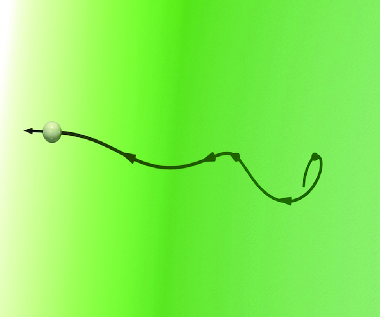

1. Introduction
Fluid homogeneity is an exception rather than the rule (More & Ardekani Reference More and Ardekani2023). Inhomogeneous fluids – those with spatial variations in properties like density, viscosity, temperature or chemical concentration – are commonly found in both nature and industry. Unlike idealised homogeneous fluids, fluids often exhibit heterogeneities that significantly affect the behaviour of particles and micro-organisms. For example, light intensity changes with depth in marine and freshwater ecosystems, chemical concentrations and temperature are not uniform in the female genital tract, density variations are found in the Earth’s atmosphere, oceans, lakes, magmas and even in cosmic gas clusters, and viscosity gradients are also frequently encountered in glaciers, magmas, blood and chemical industries. Microswimmers frequently adapt their motion in response to these fluid gradients, a behaviour known as physicotaxis. Such responses include phototaxis in light intensity gradients (Jékely et al. Reference Jékely, Colombelli, Hausen, Guy, Stelzer, Nédélec and Arendt2008; Bennett & Golestanian Reference Bennett and Golestanian2015; Giometto et al. Reference Giometto, Altermatt, Maritan, Stocker and Rinaldo2015; Lozano et al. Reference Lozano, ten Hagen, Löwen and Bechinger2016; Dai et al. Reference Dai, Wang, Xiong, Zhan, Dai, Li, Feng and Tang2016), magnetotaxis in magnetic fields (Klumpp & Faivre Reference Klumpp and Faivre2016; Rupprecht et al. Reference Rupprecht, Waisbord, Ybert, Cottin-Bizonne and Bocquet2016; Waisbord et al. Reference Waisbord, Lefèvre, Bocquet, Ybert and Cottin-Bizonne2016), chemotaxis in chemical concentration gradients (Berg & Brown Reference Berg and Brown1972; Eisenbach Reference Eisenbach1999), thermotaxis in temperature gradients (Bahat et al. Reference Bahat, Tur-Kaspa, Gakamsky, Giojalas, Breitbart and Eisenbach2003; Li et al. Reference Li, Zhao, Huang, Lin, Guo, Wang, Li, Wang and Duan2013; Bickel, Zecua & Würger Reference Bickel, Zecua and Würger2014), gravitaxis in response to gravitational potential (Campbell & Ebbens Reference Campbell and Ebbens2013; Wolff et al. Reference Wolff, Hahn and Stark2013; ten Hagen et al. Reference ten Hagen, Kümmel, Wittkowski, Takagi, Löwen and Bechinger2014; Campbell et al. Reference Campbell, Wittkowski, Ten Hagen, Löwen and Ebbens2017) and densitaxis driven by density variations (Ardekani, Doostmohammadi & Desai Reference Ardekani, Doostmohammadi and Desai2017; More & Ardekani Reference More and Ardekani2023; Shaik & Elfring Reference Shaik and Elfring2024). Physicotaxis a crucial role in many processes such as optimising nutrient uptake, avoiding toxins and guiding sperm cells towards eggs (Eisenbach & Giojalas Reference Eisenbach and Giojalas2006). The mechanisms of taxis also offer significant potential for designing microrobots with biomedical applications, including micro-cargo transport (Baraban et al. Reference Baraban, Tasinkevych, Popescu, Sanchez, Dietrich and Schmidt2011; Boymelgreen et al. Reference Boymelgreen, Balli, Miloh and Yossifon2018), targeted drug delivery (Srivastava et al. Reference Srivastava, Medina-Sánchez, Koch and Schmidt2016; Bhuyan et al. Reference Bhuyan, Singh, Dutta, Unal, Ghosh and Bandyopadhyay2017; Bunea & Taboryski Reference Bunea and Taboryski2020) and microsurgery (Nelson, Kaliakatsos & Abbott Reference Nelson, Kaliakatsos and Abbott2010; Srivastava et al. Reference Srivastava, Medina-Sánchez, Koch and Schmidt2016; Bunea & Glückstad Reference Bunea and Glückstad2019; Bunea & Taboryski Reference Bunea and Taboryski2020).
Among the various forms of fluid heterogeneity, density and viscosity stratification are particularly common. While much has been learned about the effects of density stratification on fluid motion (Ardekani et al. Reference Ardekani, Doostmohammadi and Desai2017; More & Ardekani Reference More and Ardekani2023), the movement of objects in fluids with varying viscosity – referred to as viscotaxis – remains less well understood. Investigating locomotion of chiral swimmers in such inhomogeneous fluids is essential for improving our understanding of a wide range of ecological and industrial processes. In this work, we focus on viscosity gradients found in various biological systems, such as human viscera (Wheeler et al. Reference Wheeler, Cárcamo-Oyarce, Turner, Dellos-Nolan, Co, Lehoux, Cummings, Wozniak and Ribbeck2019) and biofilms (Hall-Stoodley, Costerton & Stoodley Reference Hall-Stoodley, Costerton and Stoodley2004), which play crucial roles in mucosal barrier function (Swidsinski et al. Reference Swidsinski, Sydora, Doerffel, Loening-Baucke, Vaneechoutte, Lupicki, Scholze, Lochs and Dieleman2007) and influence cell motility (Wheeler et al. Reference Wheeler, Cárcamo-Oyarce, Turner, Dellos-Nolan, Co, Lehoux, Cummings, Wozniak and Ribbeck2019). Experimental studies reveal diverse responses to viscosity gradients. For instance, Leptospira (Kaiser & Doetsch Reference Kaiser and Doetsch1975; Petrino & Doetsch Reference Petrino and Doetsch1978; Takabe et al. Reference Takabe, Tahara, Islam, Affroze, Kudo and Nakamura2017) and Spiroplasma (Daniels, Longland & Gilbart Reference Daniels, Longland and Gilbart1980) exhibit positive viscotaxis, moving up viscosity gradients, while E. coli demonstrates negative viscotaxis, moving down these gradients (Sherman, Timkina & Glagolev Reference Sherman, Timkina and Glagolev1982). Additionally, Chlamydomonas reinhardtii displays unique behaviours: it shows negative viscotaxis in sufficiently strong gradients, accumulates in high-viscosity regions under weak gradients (Stehnach et al. Reference Stehnach, Waisbord, Walkama and Guasto2021) and scatters away from interfaces when crossing from low-viscosity to high-viscosity regions (Coppola & Kantsler Reference Coppola and Kantsler2021).
Theoretical studies have also explored both positive and negative viscotaxis (Liebchen et al. Reference Liebchen, Monderkamp, ten Hagen and Löwen2018; Datt & Elfring Reference Datt and Elfring2019; Shaik & Elfring Reference Shaik and Elfring2021; Gong, Shaik & Elfring Reference Gong, Shaik and Elfring2023, Reference Gong, Shaik and Elfring2024a ,Reference Gong, Shaik and Elfring b ). Liebchen et al. (Reference Liebchen, Monderkamp, ten Hagen and Löwen2018) investigated the viscotaxis of a dumbbell-shaped swimmer composed of two spheres, as well as a triangular swimmer composed of three spheres, each subject to a propulsion force. These models were used to represent microswimmers such as Leptospira and Spiroplasma, which exhibit positive viscotaxis (Kaiser & Doetsch Reference Kaiser and Doetsch1975; Petrino & Doetsch Reference Petrino and Doetsch1978; Daniels et al. Reference Daniels, Longland and Gilbart1980; Takabe et al. Reference Takabe, Tahara, Islam, Affroze, Kudo and Nakamura2017). Further studies examined the effects of viscosity gradients on propulsion using both spherical (Datt & Elfring Reference Datt and Elfring2019; Shaik & Elfring Reference Shaik and Elfring2021; Gong et al. Reference Gong, Shaik and Elfring2023) and spheroidal (Gong et al. Reference Gong, Shaik and Elfring2024a ,Reference Gong, Shaik and Elfring b ) squirmer models, which are modelled by squirming velocities (Lighthill Reference Lighthill1952; Blake Reference Blake1971; Ishikawa Reference Ishikawa2009; Pak & Lauga Reference Pak and Lauga2014; Pedley Reference Pedley2016; Ishikawa Reference Ishikawa2024). For a spherical squirmer, of all polar squirming modes, only the first two modes contribute to the translational and rotational velocities in the linear viscosity gradients, as derived by (Datt & Elfring Reference Datt and Elfring2019)
 \begin{align} \boldsymbol{U} & = \boldsymbol{U}_N - \frac {aB_2}{5}(\boldsymbol{1} - 3\mathbf{pp})\cdot \boldsymbol{\nabla }\left (\frac {\eta }{\eta _0}\right ),\\[-18pt]\nonumber \end{align}
 \begin{align} \boldsymbol{\Omega } & = -\frac {1}{2}\boldsymbol{U}_N\times \boldsymbol{\nabla }\left (\frac {\eta }{\eta _0}\right ), \end{align}
where
 $\boldsymbol{U}_N = (2 / 3)B_1\mathbf{p}$
is the velocity in uniform Newtonian fluids (with
 $\mathbf{p}$
representing the swimming axis),
 $a$
is the swimmer’s radius,
 $\eta _0$
is the characteristic viscosity and
 $\boldsymbol{\nabla }\eta$
is the viscosity gradient. Squirmers exhibit negative viscotaxis, with their velocities depending on their swimming mode. Interestingly, squirmers with only the
 $B_2$
mode can swim in linear viscosity gradients even without propulsion in uniform Newtonian fluids.
Chirality plays a crucial role in the locomotion of microswimmers, enabling them to convert rotational motion into translational propulsion (Yashima et al. Reference Yashima, Ousaka, Taura, Shimomura, Ikai and Maeda2016; Morrow, Bissette & Fletcher Reference Morrow, Bissette and Fletcher2017). At low Reynolds numbers, movement requires body deformations that break time-reversal symmetry (Purcell Reference Purcell1977). Many micro-organisms overcome this by dynamically altering their chiral bodies. Most micro-organisms inherently possess chirality, leading to a hydrodynamic coupling between translation and rotation motion (Keaveny & Shelley Reference Keaveny and Shelley2009; Kraft et al. Reference Kraft, Wittkowski, ten Hagen, Edmond, Pine and Löwen2013; Keaveny, Walker & Shelley Reference Keaveny, Walker and Shelley2013; Löwen Reference Löwen2016). For instance, E. coli propels itself using rotating helical flagella that leverage this coupling (Berg & Anderson Reference Berg and Anderson1973; Lauga Reference Lauga2016), while the helical body shapes of Helicobacter pylori and Campylobacter jejuni facilitate efficient swimming (Constantino et al. Reference Constantino, Jabbarzadeh, Fu and Bansil2016). More generally, chiral particles in translational motion simultaneously rotate, often following a helical trajectory (Ghosh & Fischer Reference Ghosh and Fischer2009; Friedrich & Jülicher Reference Friedrich and Jülicher2009; Su et al. Reference Su, Choi, Feng, Huang, McLeod and Ozcan2013; Namdeo, Khaderi & Onck Reference Namdeo, Khaderi and Onck2014). Helical trajectories are widely observed among micro-organisms. Notable examples include Spiroplasma (Yang, Wolgemuth & Huber Reference Yang, Wolgemuth and Huber2009), Leptospira (Berg & Anderson Reference Berg and Anderson1973), Euglena gracilis (Rossi et al. Reference Rossi, Cicconofri, Beran, Noselli and DeSimone2017) and Helicobacter pylori (Constantino et al. Reference Constantino, Jabbarzadeh, Fu and Bansil2016). Many motile cells exhibit helical swimming due to flagella exerting off-axis forces relative to the cell body, inducing wobbling motion (Hyon et al. Reference Hyon Yunkyong, Powers, Stocker and Fu2012). Understanding the role of chirality in microswimmer motility has attracted significant attention (Archer, Campbell & Ebbens Reference Archer, Campbell and Ebbens2015; Tjhung, Cates & Marenduzzo Reference Tjhung, Cates and Marenduzzo2017; Yamamoto & Sano Reference Yamamoto and Sano2017, Reference Yamamoto and Sano2018; Carenza et al. Reference Carenza, Gonnella, Marenduzzo and Negro2019; Lancia et al. Reference Lancia, Yamamoto, Ryabchun, Yamaguchi, Sano and Katsonis2019; Fadda, Molina & Yamamoto Reference Fadda, Molina and Yamamoto2020), not only for biological insights but also for potential applications in designing artificial active particles.
While experimental investigations have explored chiral microswimmers like E. coli cells, theoretical studies typically focus on microswimmers without chirality, leaving chiral swimmers less understood. Based on the current state of the literature, it is clear that further theoretical investigations are needed to deepen our understanding of how viscosity gradients influence the locomotion of chiral swimmers. In this study, we model chiral microswimmers, such as E. coli, using a squirmer with both polar and azimuthal squirming modes to investigate the effects of chirality on locomotion. The squirmer model is a well-estabilished mathematical model of microswimmers, can describe various types of swimmers, from biological micro-organisms to diffusiophoretic Janus particles, within a unified theoretical framework, and provides a versatile framework to examine the responses of different classes of microswimmers – pushers, pullers and neutral swimmers (Pedley Reference Pedley2016; Ishikawa Reference Ishikawa2024). Previous studies have shown that chirality, represented by the azimuthal squirming modes, can significantly influence swimmer behaviour. Chiral squirmers, characterised by the misalignment of source dipoles and rotlets, follow the helical paths. The hydrodynamic interactions between two such squirmers can result in attraction, repulsion and bounded states, where the swimmers oscillate around a common average trajectory (Burada, Maity & Jülicher Reference Burada, Maity and Jülicher2022). Moreover, the rotational dynamics of these chiral squirmers can exhibit synchronisation, manifesting as velocity alighment with a high degree of orientational order in both the polar and azimuthal directions (Samatas & Lintuvuori Reference Samatas and Lintuvuori2023). The rotlet dipole enhances swimming velocity in uniform viscoelastic fluids (Binagia et al. Reference Binagia, Phoa, Housiadas and Shaqfeh2020; Housiadas, Binagia & Shaqfeh Reference Housiadas, Binagia and Shaqfeh2021; Kobayashi et al. Reference Kobayashi, Jung, Matsuoka, Nakayama, Molina and Yamamoto2023, Reference Kobayashi, Molina and Yamamoto2024), while reducing it in uniform shear-thinning fluids (Nganguia et al. Reference Nganguia, Zheng, Chen, Pak and Zhu2020). Additionally, spherical microswimmers with the rotlet dipole exhibit circular trajectories on a flat wall (Fadda et al. Reference Fadda, Molina and Yamamoto2020), consistent with experimental observations of E. coli (Lauga et al. Reference Lauga, DiLuzio, Whitesides and Stone2006). Exploring chiral swimmer locomotion in viscosity gradients could offer valuable insights into cell motility in complex biological systems, but this remains an open question.
Schematic representations of (a) the motion of a squirmer with orientation
 $\mathbf{p}$
in fluids exhibiting viscosity gradients, and (b) and (c) the surface slip velocities
 $\boldsymbol{u}^{\mathcal{S}}$
corresponding to the
 $B_1$
and
 $C_2$
modes, respectively.

(a) Time evolution of the orientation
 $\mathbf{p}$
of the chiral swimmer. (b) and (c) Schematic representations of the mechanism driving the rotation, caused by the coupling between chirality and the viscosity gradient, for the (b) perpendicular (
 $\mathbf{p} \perp \boldsymbol{e}_\eta$
) and (c) parallel (
 $\mathbf{p} \parallel \boldsymbol{e}_\eta$
) cases.

In this study, we investigate the propulsion of a chiral microswimmer in a constant viscosity gradient using the canonical spherical squirmer model (Lighthill Reference Lighthill1952; Blake Reference Blake1971; Pak & Lauga Reference Pak and Lauga2014) (see figure 1 for schematic representations). We derive analytical expressions for the velocities of a single chiral microswimmer, and demonstrate that the coupling between the swimmer’s chirality and viscosity gradients leads to intriguing orientation dynamics (figure 2). These dynamics can be described by the Landau–Lifshitz–Gilbert (LLG) equations, commonly used for spin systems (Gilbert Reference Gilbert2004; Lakshmanan Reference Lakshmanan2011). Chiral microswimmers exhibit negative viscotaxis, moving towards regions of lower viscosity with spiral motions. Their trajectories transition from spiral (chiral) to straight (achiral) in viscosity gradients (figure 3). Furthermore, we show that chiral microswimmers with varying angles between the source and rotlet dipoles always spiral towards lower viscosity regions, regardless of their initial orientation. This behaviour contrasts with that of chiral swimmers with fixed dipole angles, whose trajectories depend on their initial conditions (figure 5). Our findings highlight the potential of leveraging distinct trajectories in viscosity gradients as a tool for cell sorting – a crucial method widely employed in biology and medical applications for isolating and characterising target cells (Tamura et al. Reference Tamura, Yanagawa, Sugiura, Takagi, Sumaru, Matsui and Kanamori2014; Datt & Elfring Reference Datt and Elfring2019).
Trajectories of chiral squirmers for various initial polar angles
 $\vartheta (0)$
and chiral parameters
 $\zeta = C_2 / B_1$
: (a,d)
 $\zeta = 1$
; (b,e)
 $\zeta = 3$
; and (c,f)
 $\zeta = 5$
. The viscosity gradient strengths are set to
 $\varepsilon = 0.1$
in panels (a–c) and
 $\varepsilon = 0.3$
in panels (d–f). The initial polar angles
 $\vartheta (0)$
are
 $0$
(bottom right),
 $\pi / 4$
(middle right),
 $\pi / 2$
(top),
 $3\pi / 4$
(middle left) and
 $\pi$
(bottom left), with the azimuthal angle fixed at
 $\varphi (0) = 0$
. When the swimmer’s orientation is perfectly parallel or antiparallel to the viscosity gradient axis
 $\boldsymbol{e}_\eta$
, it follows a straight trajectory. However, if the orientation deviates from the axis, the swimmer follows spiral trajectories, exhibiting negative viscotaxis.

2. Mathematical formulation
2.1. Squirmer model
We employ the squirmer model (Lighthill Reference Lighthill1952; Blake Reference Blake1971; Pak & Lauga Reference Pak and Lauga2014) to represent microswimmers, where propulsion is generated by a slip velocity at the swimmer’s surface. This model has been widely used in biological fluid mechanics to elucidate the hydrodynamics of swimming micro-organisms (Pedley Reference Pedley2016; Ishikawa Reference Ishikawa2024). Building on previous work by Datt & Elfring (Reference Datt and Elfring2019), we investigate a squirmer with complete polar and azimuthal squirming modes in viscosity gradients. The general slip velocity at the surface is given by
 \begin{align} \boldsymbol{u}^{\mathcal{S}}(\theta , \phi ) = \sum _{n = 1}^\infty \left [\frac {2}{n(n + 1)}B_nP^{\prime}_n(\cos \theta )\sin \theta \hat {\boldsymbol{\theta }} + C_nP^{\prime}_n(\cos \theta )\sin \theta \hat {\boldsymbol{\phi }}\right ], \end{align}
where
 $P^{\prime}_n$
is the derivative of the
 $n$
th-order Legendre polynomial,
 $B_n$
and
 $C_n$
are the coefficients for the
 $n$
th polar and azimuthal squirming modes, respectively, with
 $\hat {\boldsymbol{\theta }}$
and
 $\hat {\boldsymbol{\phi }}$
denoting the unit polar and azimuthal tangent vectors, respectively. The first polar and azimuthal modes,
 $B_1$
and
 $C_1$
, determine the steady swimming speed in a uniform Newtonian fluid at zero Reynolds number, given by
 $U_{N} = (2/3)B_1$
and
 $\Omega _N = -C_1 / a$
, respectively. The azimuthal squirming modes have been used to model the chirality of microswimmers (Ghose & Adhikari Reference Ghose and Adhikari2014; Pedley Reference Pedley2016; Pedley, Brumley & Goldstein Reference Pedley, Brumley and Goldstein2016). When the polar and azimuthal squirming axes are aligned, squirmers swim in straight paths with rotational velocity
 $\Omega _N$
. However, the effects of their misalignment have only recently begun to receive attention. In such cases, squirmers follow chiral (spiral) trajectories (Burada et al. Reference Burada, Maity and Jülicher2022; Samatas & Lintuvuori Reference Samatas and Lintuvuori2023). In addition to the rotlet mode
 $C_1$
, rotlet dipoles
 $C_2$
, which describe the flow pattern generated by a microswimmer with rotating flagella and a counter-rotating body, play a significant role in propulsion near walls (Fadda et al. Reference Fadda, Molina and Yamamoto2020) and in complex fluids (Binagia et al. Reference Binagia, Phoa, Housiadas and Shaqfeh2020; Nganguia et al. Reference Nganguia, Zheng, Chen, Pak and Zhu2020; Housiadas et al. Reference Housiadas, Binagia and Shaqfeh2021; Kobayashi et al. Reference Kobayashi, Jung, Matsuoka, Nakayama, Molina and Yamamoto2023, Reference Kobayashi, Molina and Yamamoto2024). In this study, we examine how chirality, represented by the full azimuthal squirming modes, influences swimming kinematics in viscosity gradients.
2.2. Fluids with viscosity gradients
The fluid is incompressible and governed by the Stokes equations:
 \begin{align} \boldsymbol{\nabla }\cdot \boldsymbol{u} = 0,\qquad \boldsymbol{\nabla }\cdot \boldsymbol{\sigma } = \boldsymbol{0}, \end{align}
where
 $\boldsymbol{u}$
and
 $\boldsymbol{\sigma }$
represent the velocity and stress fields, respectively. We investigate a Newtonian fluid with viscosity variations influenced by factors such as temperature
 $T$
(Oppenheimer, Navardi & Stone Reference Oppenheimer, Navardi and Stone2016) and nutrient concentration
 $C$
(Shoele & Eastham Reference Shoele and Eastham2018), expressed as
 $\eta = \eta (T, C)$
. Since both temperature
 $T$
and concentration
 $C$
are governed by the advection–diffusion equations, they evolve over time
 $t$
and space
 $\boldsymbol{r}$
. Consequently, viscosity fields can be written as
 $\eta = \eta [T(t, \boldsymbol{r}), C(t, \boldsymbol{r})]$
. While swimming motion can influence viscosity variations, we follow the assumptions of Oppenheimer et al. (Reference Oppenheimer, Navardi and Stone2016) and Shoele & Eastham (Reference Shoele and Eastham2018), assuming that advective transport of thermal energy and concentration is negligible compared with diffusion. Specifically, we assume that the Péclet numbers
 $\textrm{Pe}_T = Ua / \kappa _T \ll 1$
and
 $\textrm{Pe}_C = Ua/ \kappa _C \ll 1$
, where
 $U$
is the characteristic velocity, and
 $\kappa _T$
and
 $\kappa _C$
represent diffusivities of thermal energy and concentration, respectively. Under these conditions, the flow-induced distortions of the temperature and concentration fields can be ignored, allowing us to express viscosity as
 $\eta = \eta (\boldsymbol{r})$
. For the micron-scale organisms considered here, we assume that the viscosity field varies only weakly, meaning the characteristic length scale
 $L$
significantly exceeds the swimmer’s size
 $a$
 $(\varepsilon \equiv a / L \ll 1)$
, as assumed in previous studies (Oppenheimer et al. Reference Oppenheimer, Navardi and Stone2016; Shoele & Eastham Reference Shoele and Eastham2018; Liebchen et al. Reference Liebchen, Monderkamp, ten Hagen and Löwen2018; Datt & Elfring Reference Datt and Elfring2019; Shaik & Elfring Reference Shaik and Elfring2021; Gong et al. Reference Gong, Shaik and Elfring2024a
,Reference Gong, Shaik and Elfring
b
). The stress field follows the Newtonian model but incorporates a spatially varying viscosity
 $\eta (\boldsymbol{r})$
, given by
 \begin{align} \boldsymbol{\sigma } = -p\boldsymbol{1} + \eta (\boldsymbol{r})\big[\boldsymbol{\nabla }\boldsymbol{u} + (\boldsymbol{\nabla }\boldsymbol{u})^T\big]. \end{align}
Therefore, the governing equation of fluids is given by
 \begin{align} -\boldsymbol{\nabla }p + \eta (\boldsymbol{r})\boldsymbol{\nabla }^2\boldsymbol{u} + (\boldsymbol{\nabla }\eta )\cdot \big[\boldsymbol{\nabla }\boldsymbol{u} + (\boldsymbol{\nabla }\boldsymbol{u})^T\big] = \boldsymbol{0}, \end{align}
where
 $p$
is the pressure. We consider a linear viscosity gradient,
 \begin{align} \boldsymbol{\nabla }\eta = \frac {\eta _0}{L} \boldsymbol{e}_\eta = \varepsilon \frac {\eta _0}{a}\boldsymbol{e}_\eta ,\qquad \left (\varepsilon \equiv \frac {a}{L}\right ), \end{align}
with the gradient directed along
 $\boldsymbol{e}_\eta$
. We ignore thermal fluctuations, focusing only on the deterministic motion of microswimmers (Liebchen et al. Reference Liebchen, Monderkamp, ten Hagen and Löwen2018; Datt & Elfring Reference Datt and Elfring2019; Shaik & Elfring Reference Shaik and Elfring2021; Gong et al. Reference Gong, Shaik and Elfring2023, Reference Gong, Shaik and Elfring2024a
,Reference Gong, Shaik and Elfring
b
).
We employ the integral theorem to derive the swimming speed of a chiral squirmer in viscosity gradients without directly computing the flow fields (Oppenheimer et al. Reference Oppenheimer, Navardi and Stone2016; Elfring Reference Elfring2017; Shoele & Eastham Reference Shoele and Eastham2018; Masoud & Stone Reference Masoud and Stone2019; Datt & Elfring Reference Datt and Elfring2019). The integral theorem is given by
 \begin{align} -\int _{\mathcal{S}}\boldsymbol{n}\cdot \boldsymbol{\sigma }\cdot \hat {\boldsymbol{u}}\ {\textrm d}S + \int _{\mathcal{S}}\boldsymbol{n}\cdot \hat {\boldsymbol{\sigma }}\cdot \boldsymbol{u}\ {\textrm d}S = 2\int _{\mathcal{V}}[\eta (\boldsymbol{r}) -\eta _0]\boldsymbol{E}:\boldsymbol{\nabla }\hat {\boldsymbol{u}}\ {\textrm d}V, \end{align}
where
 $\mathcal{V}$
and
 $\mathcal{S}$
denote the fluid volume and the surface of the particle, respectively, and
 $\boldsymbol{n}$
is the normal surface vector directed into the fluid. As an auxiliary problem, we consider
 $\hat {\boldsymbol{u}}$
and
 $\hat {\boldsymbol{\sigma }}$
, which satisfy the Stokes equation with constant viscosity
 $\eta _0$
.
3. Swimming speeds of chiral squirmers in viscosity gradients
We solve the swimming problem using a regular perturbation expansion of
 $\varepsilon$
, expressed as
 \begin{align} \{\boldsymbol{u},\boldsymbol{\sigma }\} =\{\boldsymbol{u}_0,\boldsymbol{\sigma }_0\} + \varepsilon \{\boldsymbol{u}_1,\boldsymbol{\sigma }_1\}+\mathcal{O}(\varepsilon ^2). \end{align}
Applying this perturbation expansion of
 $\varepsilon$
to the integral theorem for Newtonian fluids with viscosity gradients (2.6), we obtain
 \begin{align} -\int _{\mathcal{S}}\boldsymbol{n}\cdot \boldsymbol{\sigma }\cdot \hat {\boldsymbol{u}}\ {\textrm d}S + \int _{\mathcal{S}}\boldsymbol{n}\cdot \hat {\boldsymbol{\sigma }}\cdot \boldsymbol{u}\ {\textrm d}S = 2\varepsilon \int _{\mathcal{V}}\eta _1\boldsymbol{E}_0:\boldsymbol{\nabla }\hat {\boldsymbol{u}}\ {\textrm d}V, \end{align}
where
 ${\boldsymbol{E}}_0$
is the strain-rate tensor corresponding to the zeroth-order velocity
 $\boldsymbol{u}_0$
, which corresponds to the solution for the uniform Stokes flow. To derive the swimming speeds of chiral squirmers, we use (3.2) and consider the auxiliary problem of a no-slip passive particle, denoted with the hat. The boundary condition for an active particle (a squirmer) is
 \begin{align} \boldsymbol{u}|_{r = a} = \boldsymbol{U} + a\boldsymbol{\Omega }\times \boldsymbol{n} + \boldsymbol{u}^{\mathcal{S}}. \end{align}
Using (3.2)–(3.3) and imposing the force-free and torque-free conditions on the squirmer, we obtain the swimming velocities,
 \begin{align} \boldsymbol{U} & = -\frac {1}{4\pi a^2}\int _{\mathcal{S}}\boldsymbol{u}^{\mathcal{S}}\ {\textrm d}S - \frac {\varepsilon }{3\pi \eta _0 a}\int _{\mathcal{V}}\eta _1\boldsymbol{E}_0:\boldsymbol{\nabla }\hat {\boldsymbol{L}}^U\ {\textrm d}V,\\[-10pt]\nonumber \end{align}
 \begin{align}\boldsymbol{\Omega } & = -\frac {3}{8\pi a^3}\int _{\mathcal{S}}\boldsymbol{n}\times \boldsymbol{u}^{\mathcal{S}}\ {\textrm d}S -\frac {\varepsilon }{4\pi \eta _0 a^3}\int _{\mathcal{V}}\eta _1\boldsymbol{E}_0:\boldsymbol{\nabla }\hat {\boldsymbol{L}}^\Omega \ {\textrm d}V, \end{align}
where
 \begin{align} \hat {\boldsymbol{L}}^{U} = \frac {3}{4}a\left (\frac {\boldsymbol{1}}{r} + \frac {\boldsymbol{nn}}{r}\right ) + \frac {1}{4}a^3\left (\frac {\boldsymbol{1}}{r^3}-\frac {3\boldsymbol{nn}}{r^3}\right ),\qquad \hat {\boldsymbol{L}}^\Omega = \left (\frac {a}{r}\right )^3\boldsymbol{\epsilon }\cdot \boldsymbol{r}, \end{align}
with
 $\boldsymbol{\epsilon }$
denoting the Levi–Civita tensor. The first terms of translational and angular velocities correspond to the swimming speed of a squirmer in the homogeneous Newtonian fluid at zero Reynolds number (the zeroth-order solution). The zeroth-order swimming velocities are
 $\boldsymbol{U}_0 = \boldsymbol{U}_N = (2 / 3)B_1\mathbf{p}$
and
 $\boldsymbol{\Omega }_0= -(C_1 / a)\mathbf{p}$
with the swimming axis
 $\mathbf{p}$
. The zeroth-order solution for
 $\boldsymbol{u}_0$
is given as (Pak & Lauga Reference Pak and Lauga2014; Lauga Reference Lauga2020)
 \begin{align} \boldsymbol{u}_0 &= u_r\boldsymbol{e}_r + u_\theta \boldsymbol{e}_\theta + u_\phi \boldsymbol{e}_\phi , \end{align}
 \begin{align} u_r &= \frac {2}{3}B_1\left (\frac {a}{r}\right )^3\cos \theta + \sum _{n =2}^\infty B_n\left [\left (\frac {a}{r}\right )^{n + 2} - \left (\frac {a}{r}\right )^n\right ]P_n(\cos \theta ), \end{align}
 \begin{align} u_\theta &=\frac {B_1}{3}\left (\frac {a}{r}\right )^3\sin \theta + \sum _{n = 2}^\infty \frac {2}{n(n + 1)}B_n\left [\frac {n}{2}\left (\frac {a}{r}\right )^{n + 2} + \left (1 - \frac {n}{2}\right )\left (\frac {a}{r}\right )^n\right ]P^{\prime}_n(\cos \theta )\sin \theta , \end{align}
 \begin{align} u_\phi &= \sum _{n = 2}^\infty C_n\left (\frac {a}{r}\right )^{n + 1}P^{\prime}_n(\cos \theta )\sin \theta . \end{align}
3.1. Alignment of the polar and azimuthal squirming axes
We now derive the translational and angular velocities
 $(\boldsymbol{U}, \boldsymbol{\Omega })$
for squirmers with all polar and azimuthal squirming modes in linear viscosity fields up to
 $\mathcal{O}(\varepsilon )$
,
 \begin{align} \boldsymbol{U} & = \frac {2}{3}B_1\mathbf{p} - \frac {aB_2}{5}(\boldsymbol{1} - 3\mathbf{pp})\cdot \boldsymbol{\nabla }\left (\frac {\eta }{\eta _0}\right ),\\[-10pt]\nonumber \end{align}
 \begin{align} \boldsymbol{\Omega } & =-\frac {C_1}{a}\mathbf{p} -\frac {B_1}{3}\mathbf{p}\times \boldsymbol{\nabla }\left (\frac {\eta }{\eta _0}\right ) + \frac {2}{5}C_2(\boldsymbol{1}-3\mathbf{pp})\cdot \boldsymbol{\nabla }\left (\frac {\eta }{\eta _0}\right ). \end{align}
Datt & Elfring (Reference Datt and Elfring2019) showed that among all polar squirming modes
 $B_n$
, only the first two modes contribute to the translational (second term in (3.7a
)) and rotational velocities (second term in (3.7b
)) in the linear gradients. The first polar mode
 $B_1$
causes the squirmer to rotate towards regions of lower viscosity (negative viscotaxis) when not perfectly aligned with the viscosity gradient (Datt & Elfring Reference Datt and Elfring2019). In this study, we find that among all azimuthal squirming modes, only the second mode
 $C_2$
contributes to the rotational velocity in the linear viscosity gradients. Therefore, we focus exclusively on the first polar mode
 $B_1$
and the second azimuthal mode
 $C_2$
, as the coupling between viscosity gradients and the swimmer’s chirality arises solely from the rotlet dipole mode
 $C_2$
.
The angular velocity due to the squirmer with
 $B_1$
and
 $C_2$
modes in the linear viscosity gradient can be decomposed by
 \begin{align} \boldsymbol{\Omega } & = \Omega _{\textit{Sp}} (\boldsymbol{e}_\eta \cdot \mathbf{p})\mathbf{p} + \Omega _{{ Pr}}\boldsymbol{e}_\eta + \Omega _{\textit{Da}}\boldsymbol{e}_\eta \times \mathbf{p},\nonumber\\[5pt] \Omega _{\textit{Sp}} & = -\frac {6C_2}{5L},\quad \Omega _{\textit{Pr}} = \frac {2C_2}{5L},\quad \Omega _{\textit{Da}} = \frac {B_1}{3L}. \end{align}
Using (3.8) and
 $\dot {\mathbf{p}} = \boldsymbol{\Omega }\times \mathbf{p}$
, we derive the orientational dynamics of the chiral squirmer (see figure 2
a), governed by the Landau–Lifshitz–Gilbert (LLG) equation, capturing the essential physics of the alignment behaviour (Gilbert Reference Gilbert2004; Lakshmanan Reference Lakshmanan2011)
 \begin{align} \dot {\mathbf{p}} = \Omega _{\textit{Pr}}(\boldsymbol{e}_\eta \times \mathbf{p}) + \Omega _{\textit{Da}}(\boldsymbol{e}_\eta \times \mathbf{p})\times \mathbf{p}. \end{align}
The swimmer exhibits damping (
 $\Omega _{\textit{Da}}$
) leading to negative viscotaxis, spinning (
 $\Omega _{\textit{Sp}}$
) around the propulsion axis
 $\mathbf{p}$
and precession (
 $\Omega _{\textit{Pr}}$
) around the axis of viscosity gradients
 $\boldsymbol{e}_\eta$
.
Interestingly, the orientation dynamics of achiral squirmers in chiral fluids with odd viscosity is governed by the fixed LLG equation, exhibiting parallel or antiparallel alignments with the axis of odd viscosity (Hosaka et al. Reference Hosaka, Chatzittofi, Golestanian and Vilfan2024). The interplay between a polar vector (orientation) and a pseudovector (axis of odd viscosity) makes parallel and antiparallel alignments equivalent. In spin systems, however, parallel and antiparallel alignments are not equivalent, as both magnetisation (or spin) and the magnetic field are pseudovectors. In viscosity gradients, both the orientation
 $\mathbf{p}$
and
 $\boldsymbol{e}_\eta$
are polar vectors, rendering parallel and antiparallel alignments non-equivalent. Consequently, the orientation dynamics can be elegantly described by the LLG equation. Moreover, while experiments on microswimmers in fluids with odd viscosity remain elusive, numerous studies on viscosity gradients (Kaiser & Doetsch Reference Kaiser and Doetsch1975; Petrino & Doetsch Reference Petrino and Doetsch1978; Daniels et al. Reference Daniels, Longland and Gilbart1980; Sherman et al. Reference Sherman, Timkina and Glagolev1982; Takabe et al. Reference Takabe, Tahara, Islam, Affroze, Kudo and Nakamura2017; Stehnach et al. Reference Stehnach, Waisbord, Walkama and Guasto2021; Coppola & Kantsler Reference Coppola and Kantsler2021) suggest our findings are experimentally reproducible.
The intriguing orientation dynamics can be understood by examining the effect of the viscosity gradient on the thrust torque. The thrust torque, generated by the slip velocity at the squirmer’s surface, dominates in regions of higher viscosity. As shown in figures 2(b) and 2(c), when the swimming axis is perpendicular (antiparallel) to the viscosity gradient, the torque is predominantly governed by the traction generated by the right (lower) hemisphere, leading to rotating around
 $\boldsymbol{e}_\eta$
(
 $\mathbf{p}$
). When not perfectly aligned with the viscosity gradient, chiral squirmers move towards regions of lower viscosity, following spiral paths. Once aligned with the viscosity gradient, the squirmer swims in a straight line with spinning. Chiral squirmers typically transition from chiral (spiral) to achiral trajectories (linear trajectories with spinning) unless perfectly aligned with viscosity gradients.
Now, we describe the swimmer’s rotation using the polar angle
 $\vartheta$
, measured from the
 $\boldsymbol{e}_\eta$
-axis, meaning
 $\vartheta = \cos ^{-1}(\mathbf{p}\cdot \boldsymbol{e}_\eta )$
, and the azimuthal angle
 $\varphi$
. The swimming axis is
 $\mathbf{p} = (\sin \vartheta \cos \varphi , \sin \vartheta \sin \varphi , \cos \vartheta )$
, and (3.9) becomes
 \begin{align} \dot {\vartheta } = \Omega _{\textit{Da}}\sin \vartheta ,\qquad \dot {\varphi } = \Omega _{\textit{Pr}}. \end{align}
The dynamics of
 $\vartheta$
are characterised by one unstable fixed point at
 $\vartheta = 0$
(corresponding to positive viscotaxis) and one stable fixed point at
 $\vartheta = \pi$
(corresponding to negative viscotaxis). Equation (3.10) solves to
 \begin{align} \tan \frac {\vartheta (t)}{2} = \tan \frac {\vartheta (0)}{2}e^{\Omega _{\textit{Da}}t},\quad \varphi (t) = \Omega _{\textit{Pr}}t + \varphi (0). \end{align}
We can estimate the characteristic time scales as follows. First, the time scale for the transition from spiral to linear trajectories corresponds to the time required for the orientation to become perfectly anti-aligned with the viscosity gradients. This time scale is governed solely by the strength of the source dipole
 $B_1$
and the viscosity gradients
 $\varepsilon$
, and is given by
 $\tau \sim 1 / \Omega _{\textit{Da}}$
. Second, the time scale associated with the spiral trajectory – specifically, the period of the helix – is determined by the strength of the rotlet dipole
 $C_2$
and the viscosity gradients
 $\varepsilon$
, and is given by
 $\tau = 2\pi / (\Omega _{\textit{Pr}}\sin \theta )$
.
We demonstrate negative viscotaxis, accompanied by spiral trajectories, for various chiral parameters
 $\zeta = C_2 / B_1$
and initial polar angles
 $\vartheta (0)$
in figure 3. Chirality allows the swimmer to follow a three-dimensional trajectory, in contrast to an achiral swimmer, which moves within a two-dimensional plane (Datt & Elfring Reference Datt and Elfring2019). As shown in figure 3, the specific trajectories vary depending on the swimmer’s chirality, orientation and viscosity gradient strengths. When the swimmer’s orientation is parallel or antiparallel to the axis of viscosity gradients
 $\boldsymbol{e}_\eta$
, it swims in a straight line. In contrast, all chiral squirmers follow spiral trajectories and exhibit negative viscotaxis unless perfectly aligned with the axis of viscosity gradients. Eventually, the swimmer will align perfectly with
 $-\boldsymbol{e}_\eta$
and exhibit straight-line motion. Particularly, the angular velocity associated with precession
 $\Omega _{\textit{Pr}}$
increases with the chiral parameter
 $\zeta$
, resulting in smaller radii for the spiral trajectories. Additionally, stronger viscosity gradients lead to larger angular velocities associated with both precession and damping, resulting in tighter spiral trajectories. These distinctions in trajectories could potentially be exploited for sorting swimmers (Tamura et al. Reference Tamura, Yanagawa, Sugiura, Takagi, Sumaru, Matsui and Kanamori2014). Furthermore, the swimmer’s paths could be used to measure the fluid’s viscosity gradient strengths.
To evaluate the impact of swimmer’s chirality, represented by the rotlet dipole, we estimate the chiral parameter
 $\zeta = C_2 / B_1$
for E. coli, which propels itself using a rotating flagellum and a counter-rotating body. Here,
 $B_1$
can be determined from the Newtonian swimming speed, given by
 $U_N =(2/3)B_1$
(Lighthill Reference Lighthill1952; Blake Reference Blake1971), where
 $U_N =$
 $8.3$
µm s
 $^{-1}$
(Patteson et al. Reference Patteson, Gopinath, Goulian and Arratia2015). To compute the chiral parameter
 $\zeta$
, we estimate
 $C_2$
based on the motion of E. coli’s helical flagellum, which spins at
 $100$
Hz with a helical diameter of
 $0.5$
µm (Lauga Reference Lauga2016). This analysis yields
 $\zeta \approx 4.0$
(Binagia et al. Reference Binagia, Phoa, Housiadas and Shaqfeh2020), suggesting that chirality plays a crucial role in the dynamics of chiral swimmers in viscosity gradients, as seen in figure 3.
Orientation of a chiral swimmer (sphere) with a misalignment between source and rotlet dipoles within the body-fixed frame
 $(\boldsymbol{e}_1,\boldsymbol{e}_2,\boldsymbol{e}_3)$
. The rotlet dipole, oriented along the
 $\mathbf{d}$
direction, forms an angle
 $\gamma$
with the swimming axis
 $\mathbf{p}$
. The body-fixed frame
 $(\boldsymbol{e}_1, \boldsymbol{e}_2, \boldsymbol{e}_3)$
(red axes) is related to the laboratory frame
 $(\boldsymbol{e}_x, \boldsymbol{e}_y, \boldsymbol{e}_z)$
(black axes) through the Euler angles
 $(\varphi , \vartheta , \psi )$
. Without loss of generality, we set
 $\boldsymbol{e}_\eta = \boldsymbol{e}_z$
and
 $\mathbf{p} = \boldsymbol{e}_3$
.

3.2. Misalignment of the polar and azimuthal squirming axes
Ciliated microorganisms generally exhibit not only translational motion, but also body rotation, resulting in helical trajectories (Crenshaw Reference Crenshaw1989). Pak & Lauga (Reference Pak and Lauga2014) introduced a general squirmer model that includes non-axisymmetric squirming motion, while Maity & Burada (Reference Maity and Burada2019) proposed the chiral squirmer, which explicitly incorporates body rotation. Burada et al. (Reference Burada, Maity and Jülicher2022) and Samatas & Lintuvuori (Reference Samatas and Lintuvuori2023) identified intriguing hydrodynamic interactions in chiral squirmers, charactrised by a deterministic misalignment of source dipoles
 $B_1$
and rotlets
 $C_1$
, distinguishing them from achiral squirmers. Next, we employ their chiral squirmer models, which incorporate misaligned polar and azimuthal squirming modes (Burada et al. Reference Burada, Maity and Jülicher2022; Maity & Burada Reference Maity and Burada2019, Reference Maity and Burada2022a
,Reference Maity and Burada
b
, Reference Maity and Burada2023; Samatas & Lintuvuori Reference Samatas and Lintuvuori2023), to investigate the behaviour of chiral squirmers in viscosity gradients. Specifically, we examine a chiral swimmer with a deterministic misalignment between the source dipole
 $B_1$
and rotlet dipole
 $C_2$
. The rotlet dipole is oriented along the
 $\mathbf{d}$
axis (blue axis in figure 4) in the body frame, forming an angle
 $\gamma$
with the swimming axis
 $\mathbf{p}$
. This configuration can resemble E. coli’s misaligned axes of propulsion and rotation of flagella and body in E. coli during its tumbling state (Macnab Reference Macnab1977). While E. coli’s tumbling is a stochastic process, our deterministic chiral squirmer model, defined by the misalignment of polar and azimuthal modes, offers fresh insights into the underlying mechanisms of E. coli’s behaviour in viscosity gradients.
We solve for the velocities in linear viscosity fields up to
 $\mathcal{O}(\varepsilon )$
,
 \begin{align} \boldsymbol{\Omega } = \Omega _{\textit{Sp}}(\boldsymbol{e}_\eta \cdot \mathbf{d})\mathbf{d} + \Omega _{\textit{Pr}}\boldsymbol{e}_\eta + \Omega _{\textit{Da}}\boldsymbol{e}_\eta \times \mathbf{p}. \end{align}
To describe the orientational dynamics of a chiral microswimmer with a misalignment between the source and rotlet dipoles, it is convenient to work in a body-fixed coordinate system with the basis
 $(\boldsymbol{e}_1, \boldsymbol{e}_2, \boldsymbol{e}_3)$
, chosen such that
 $\boldsymbol{e}_3 \equiv \mathbf{p}$
. The swimmer’s orientation relative to the laboratory frame – defined by the basis
 $(\boldsymbol{e}_x, \boldsymbol{e}_y, \boldsymbol{e}_z)$
, where
 $\boldsymbol{e}_z \equiv \boldsymbol{e}_\eta$
– is described using the Euler angles
 $(\varphi , \vartheta , \psi )$
. Here,
 $\varphi$
and
 $\vartheta$
denote the azimuthal and polar angles measured from the
 $\boldsymbol{e}_z = \boldsymbol{e}_\eta$
axis, and
 $\psi$
represents the roll angle about the direction
 $\mathbf{p}$
(see figure 4). As shown in figure 4, the rotation follows the
 $zxz$
-convention, consisting of a rotation by
 $\varphi$
about
 $\boldsymbol{e}_z$
, followed by a rotation by
 $\vartheta$
about the
 $x$
axis of the newly obtained frame (indicated by the green arrow in figure 4) and, finally, a rotation by
 $\psi$
about the body fixed axis
 $\boldsymbol{e}_3$
. The rotation matrix
 $\mathbf{R}$
that transforms the laboratory frame basis vectors to the body-fixed basis vectors is given by
 \begin{align} \mathbf{R} = \left (\!\!\! \begin{array}{ccc} \cos \varphi \cos \psi - \sin \varphi \cos \vartheta \sin \psi &\!\! \sin \varphi \cos \psi + \cos \varphi \cos \vartheta \sin \psi &\!\! \sin \vartheta \sin \psi \\ -\cos \varphi \sin \psi - \sin \varphi \cos \vartheta \cos \psi &\!\! -\sin \varphi \sin \psi + \cos \varphi \cos \vartheta \cos \psi &\!\! \sin \vartheta \cos \psi \\ \sin \varphi \sin \vartheta &\!\! -\cos \varphi \sin \vartheta &\!\! \cos \vartheta \end{array}\!\!\! \right ) \end{align}
The inverse transformation is given by
 \begin{align} (\boldsymbol{e}_x, \boldsymbol{e}_y, \boldsymbol{e}_z) = \mathbf{R}^T\cdot (\boldsymbol{e}_1, \boldsymbol{e}_2, \boldsymbol{e}_3). \end{align}
We can express the axis of viscosity gradients as
 $\boldsymbol{e}_\eta = \sin \vartheta \sin \psi \boldsymbol{e}_1 + \sin \vartheta \cos \psi \boldsymbol{e}_2 + \cos \vartheta \boldsymbol{e}_3$
. The angular velocity of the swimmer can be expressed in terms of the derivatives of the Euler angles as
 \begin{align} \boldsymbol{\Omega } = (\dot {\varphi }\sin \vartheta \sin \psi + \dot {\vartheta }\cos \psi )\boldsymbol{e}_1 + (\dot {\varphi } \sin \vartheta \cos \psi - \dot {\vartheta }\sin \psi )\boldsymbol{e}_2 + (\dot {\varphi } \cos \vartheta + \dot {\psi })\boldsymbol{e}_3. \end{align}
By representing
 $\mathbf{d} = \sin \gamma \boldsymbol{e}_1 + \cos \gamma \boldsymbol{e}_3$
without loss of generality, and substituting into (3.12), we obtain
 \begin{align} \boldsymbol{\Omega } &= \Omega _{\textit{Sp}}(\sin \gamma \sin \vartheta \sin \psi + \cos \gamma \cos \vartheta )(\sin \gamma \boldsymbol{e}_1 + \cos \gamma \boldsymbol{e}_3) \nonumber\\&\quad + \Omega _{\textit{Pr}}(\sin \vartheta \sin \psi \boldsymbol{e}_1 + \sin \vartheta \cos \psi \boldsymbol{e}_2 + \cos \vartheta \boldsymbol{e}_3) \nonumber\\ &\quad + \Omega _{\textit{Da}}(\sin \vartheta \cos \psi \boldsymbol{e}_1 - \sin \vartheta \sin \psi \boldsymbol{e}_2). \end{align}
Equating the two expressions for the angular velocity ((3.15) and (3.16)), we obtain the following equations:
 \begin{align} \dot {\varphi } & = \Omega _{\textit{Sp}}\sin \gamma \sin \psi \left (\sin \gamma \sin \psi + \frac {\cos \gamma }{\tan \vartheta }\right ) + \Omega _{\textit{Pr}},\\[-10pt]\nonumber \end{align}
 \begin{align} \dot {\vartheta } & = \Omega _{\textit{Sp}}\sin \gamma \cos \psi (\sin \gamma \sin \vartheta \sin \psi + \cos \gamma \cos \vartheta )+ \Omega _{\textit{Da}}\sin \vartheta ,\\[-10pt]\nonumber \end{align}
 \begin{align}\dot {\psi } & = \Omega _{\textit{Sp}}\left (\cos ^2\gamma \cos \vartheta - \sin ^2\gamma \cos \vartheta \sin ^2\psi + \sin \gamma \cos \gamma \frac {\sin ^2\vartheta - \cos ^2\vartheta }{\sin \vartheta }\sin \psi \right ). \end{align}
Since the equations are independent of
 $\varphi$
, it suffices to examine the phase portraits in the
 $(\vartheta ,\psi )$
plane (see figure 5
d–f). The system displays a spiral source and sink, with the sink indicating negative viscotaxis. At the steady state, the axis of angular velocity
 $\boldsymbol{\Omega }$
is nearly antiparallel to the axis of viscosity gradients (see figure 5
a–c). Consequently, the steady-state trajectories of chiral squirmers are spiral, with the radius of these spiral trajectories decreasing with the angle
 $\gamma$
(see figure 5
g). Swimmers with
 $\mathbf{d} \ne \mathbf{p}$
consistently exhibit spiral trajectories, unlike swimmers with
 $\mathbf{d} = \mathbf{p}$
. Furthermore, the unstable point, which corresponds to the positive viscotaxis for swimmers with
 $\mathbf{d}=\mathbf{p}$
, disappears for swimmers with
 $\mathbf{d}\ne \mathbf{p}$
. Additionally, increasing the chiral parameters
 $\zeta$
results in a smaller radius, while increasing the viscosity gradients
 $\varepsilon$
leads to tighter spiral trajectories. We can estimate the characteristics time scale for the spiral, specifically the period of the helix. Since the axis of angular velocity
 $\boldsymbol{\Omega }$
is nearly antiparallel to
 $\mathbf{d}$
, the period can be approximated as
 $\tau \sim 2\pi / (\Omega \sin \gamma )$
, with
 $\Omega = |\boldsymbol{\Omega }|$
.
(a)–(c) Schematic representations of a chiral swimmer’s steady-state orientation for different angles: (a)
 $\gamma = \pi / 8$
, (b)
 $\gamma = \pi / 4$
and (c)
 $\gamma = 3\pi / 8$
, with fixed parameters
 $\varepsilon = 0.1$
and
 $\zeta = 5$
. (d)–(f) Phase portraits of the orientational dynamics of a chiral squirmer for various angles: (d)
 $\gamma = \pi / 8$
, (e)
 $\gamma = \pi / 4$
and (f)
 $\gamma = 3\pi / 8$
, with
 $\varepsilon = 0.1$
and
 $\zeta = 5$
. Each phase portrait shows one spiral source (white circle) and one spiral sink (black circle), with red lines representing example trajectories. (g) Steady-state trajectories of swimmers for different angles
 $\gamma$
. All swimmers exhibit negative viscotaxis.

4. Conclusion
We present analytical expressions for the velocities of chiral microswimmers in viscosity gradients. The interaction between the swimmer’s chirality and the fluid’s viscosity gradient induces an additional rotation described by the Landau–Lifshitz–Gilbert (LLG) equations. Squirmers exhibit three key dynamics: damping (
 $\Omega _{\textit{Da}}$
), associated with negative viscotaxis; spinning (
 $\Omega _{\textit{Sp}}$
) around the propulsion axis
 $\mathbf{p}$
; and precession (
 $\Omega _{\textit{Pr}}$
) around the viscosity gradient axis
 $\boldsymbol{e}_\eta$
. Similar orientation behaviours are observed in achiral swimmers within chiral fluids, such as those with odd viscosity (Hosaka et al. Reference Hosaka, Chatzittofi, Golestanian and Vilfan2024), indicating that both swimmer and fluid chirality can generate chiral motion. Notably, chiral squirmers with misaligned dipoles (
 $\mathbf{d}\ne \mathbf{p}$
) follow steady-state spiral trajectories aligned with negative viscotaxis.
Several theoretical studies have explored the behaviour of microswimmers in sharp viscosity gradients (Esparza López et al. Reference Esparza López, Gonzalez-Gutierrez, Solorio-Ordaz, Lauga and Zenit2021; Feng et al. Reference Feng, Molina, Turner and Yamamoto2023; Gong et al. Reference Gong, Shaik and Elfring2023; Das Reference Das2023). Esparza López et al. (Reference Esparza López, Gonzalez-Gutierrez, Solorio-Ordaz, Lauga and Zenit2021) investigated a helical swimmer crossing viscosity gradients while accounting for gravitational forces. The theoretical predictions of Gong et al. (Reference Gong, Shaik and Elfring2023), based on the squirmer model, align with experimental observations of Chlamydomonas Reinhardtii algae (Coppola & Kantsler Reference Coppola and Kantsler2021). Feng et al. (Reference Feng, Molina, Turner and Yamamoto2023) found that the swimming dynamics at an interface with a viscosity difference are strongly influenced by the incoming angle, viscosity ratio and swimming type (i.e. pusher, puller or neutral squirmer). This leads to four distinct dynamical modes: bouncing, sliding, penetrating and hovering. These behaviours have not been observed in linear viscosity gradients. However, squirmers generally reorient towards the lower viscosity region (Feng et al. Reference Feng, Molina, Turner and Yamamoto2023; Gong et al. Reference Gong, Shaik and Elfring2023), consistent with findings in linear viscosity gradients (Datt & Elfring Reference Datt and Elfring2019). Das (Reference Das2023) considered point-like variations of viscosity and provided a corresponding Green’s function for this scenario. Exploring the dynamics of a chiral squirmer near viscosity interfaces and in fluids with rapidly varying viscosity presents a promising avenue for future research, which we intend to pursue.
Theoretical predictions of active particle trajectories open new avenues for designing and fabricating artificial microswimmers with precisely controlled trajectories, particularly self-diffusiophoretic Janus particles (Anderson Reference Anderson1989). The ability to regulate particle velocities is crucial for enhancing cargo binding efficiency (van Reenen et al. Reference van, Alexander, Arthur and Prins2013). Recent experimental (Archer et al. Reference Archer, Campbell and Ebbens2015) and theoretical studies (Lisicki, Reigh & Lauga Reference Lisicki, Reigh and Lauga2018) provide a promising foundation for practical applications of chiral swimmers. Furthermore, our results on the helical motion of chiral swimmers in viscosity gradients offer new insights into optimising active particle design. Additionally, the observed spiral motion of charged particles in constant magnetic fields (Lluis González et al. Reference Lluis González, Salinas Delgado and Cabo Montes de Oca2022) may provide further analogies to our findings.
Future studies will explore not only single-swimmer phenomena, such as traction-driven microswimmers (Hosaka, Golestanian & Vilfan Reference Hosaka, Golestanian and Vilfan2023; Ishikawa Reference Ishikawa2024; Kobayashi & Yamamoto Reference Kobayashi and Yamamoto2024) and viscoelastic effects (durotaxis) (Shaik et al. Reference Shaik, Gong and J Elfring2024), but also collective behaviours of chiral microswimmers (Samatas & Lintuvuori Reference Samatas and Lintuvuori2023) in viscosity gradients. Levis, Pagonabarraga & Liebchen (Reference Levis, Pagonabarraga and Liebchen2019) suggested that chiral activity can induce synchronisation, while Ventejou et al. (Reference Ventejou, Chaté, Montagne and Shi2021) demonstrated that the homogeneous synchronised state is typically linearly unstable. An open question remains in the numerical simulations of chiral active particles with hydrodynamic interactions, which could bridge the gap between dry minimal models and experimental studies on suspensions of sperm cells and bacteria (Liebchen & Levis Reference Liebchen and Levis2022). With similarity to the Vicsek model (Vicsek et al. Reference Vicsek, Czirók, Ben-Jacob, Cohen and Shochet1995), where the orientations are governed by the XY model for spin systems, our findings on orientation dynamics (LLG equation) offer valuable insights into the connections between active matter and spin systems. The transition mechanisms we identify offer insights into the diverse swimming behaviours influenced by fluid rheology, such as E. coli’s run-and-tumble motion (Kurzthaler et al. Reference Kurzthaler2024) or mammalian sperm chemokinetics (Zaferani & Abbaspourrad Reference Zaferani and Abbaspourrad2023). Finally, our results could inform the development of tools (Tamura et al. Reference Tamura, Yanagawa, Sugiura, Takagi, Sumaru, Matsui and Kanamori2014) for cell sorting and quantifying viscosity gradients in complex fluids.
Acknowledgements
We thank Norihiro Oyama for his careful reading of the manuscript and constructive comments. We also thank Raymond E. Goldstein, Ronojoy Adhikari, Mitsusuke Tarama and Yuto Hosaka for fruitful discussions. We also would like to acknowledge the anonymous referees for their valuable feedback and constructive criticism, which improve the quality of this work.
Funding
This work was supported by the Grants-in-Aid for Scientific Research (JSPS KAKENHI) under Grant Number 20H05619, by the JSPS Core-to-Core Program ‘Advanced core-to-core network for the physics of self-organising active matter (JPJSCCA20230002)’ and by JST SPRING, Grant Number JPMJSP2110.
Declaration of interests
The authors report no conflict of interest.



