
I. INTRODUCTION
Molecular dynamics (MD), the numerical solution of atomistic equations of motion, is an established workhorse in the computational physical sciences. Its popularity—as of 2017, more than 3 million papers refer to MD—relies on its predictive power: because MD generates an unbiased sample from the ensemble of valid trajectories given some dynamics and some initial conditions, they can, in principle, be used to compute any thermodynamic, or perhaps even more importantly, dynamic quantity of interest. These remarkable advantages, however, come at a rather steep computational price that often prohibits direct simulations in relevant experimental regimes of size, time, temperature, strain rate, etc. An important cause of this limitation is rooted in constraints imposed by the complex, multiscale nature of the potential energy surface, i.e., the (3N + 1)-dimensional surface that assigns a potential energy to every point in configuration space. In the case of hard materials, such a surface is typically composed of a very large number of local minima, separated from one another by energetic and/or entropic barriers. In this setting, the maximum integration time step dt has to be a small fraction of the period of the fastest vibrational mode of the system (which is controlled by the highest curvature around minima; for hard materials dt ∼ 1 fs). On the other hand, “interesting” trajectories for materials science application should capture micro/nano-structural evolution; i.e., they should contain many jumps from one basin to another. The so-called timescale problem of MD stems from the fact that jumps between basins occur on timescales that can be exponentially longer than vibrational timescales, especially at low temperatures. For example, escape from basins can require nanoseconds to seconds, which implies 106–1015 time steps, and hence this many evaluations of the forces on each atom in the system (which is by far the most computationally intensive operation in MD). Even when the basin-to-basin transitions are fast, complex evolution might involve very large numbers of transitions, which again require very large numbers of force calls to observe.
While executing MD in serial is extremely limiting, colossal parallel computing resources are increasingly available: we are now squarely in the petascale era [where computers can carry out 1015 floating point operations per second (flops)] and the exascale era is looming (where computers will carry out 1018 flops). The challenge with leveraging these machines efficiently is that their computing power is provided by a large number of processing elements (up to millions in current machines). Therefore, whether an MD simulation of a given size and duration is possible depends on two factors: (i) an actual computer that provides enough flops to carry out the simulation in a reasonable amount of time is available and (ii) an algorithm that can efficiently exploit that computer’s architecture is available.
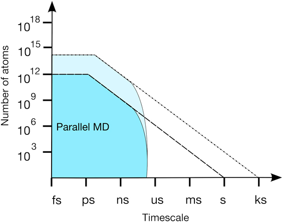
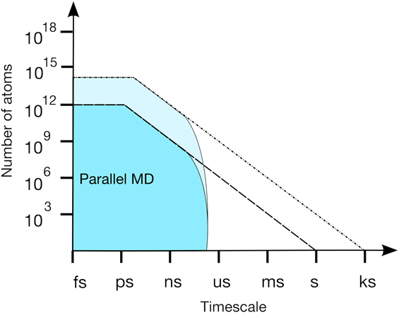
Even when requirement (i) is fulfilled, requirement (ii) can be challenging because integrating a differential equation is inherently a serial task: time step i has to be completed before time step i + 1 can be initiated. (Note that some algorithms relax that requirement when a cheaper surrogate model is available.Reference Lions, Maday and Turinici1) Therefore, to first order, the generation of a phase-space continuous MD trajectory can only be parallelized within individual time steps, not across time steps. The most common approach to parallelizing MD is through domain (or spatial) decomposition, where the simulation domain is partitioned into regions that are assigned to different computing elements. These elements are responsible for (i) computing the forces and (ii) for time stepping the atoms in their domain. Task (i) requires knowing where atoms outside the boundaries of the domain are located; i.e., it requires communication between neighboring domains. For short-ranged potentials, domain decomposition is therefore scalable in the weak-scaling mode; i.e., parallel efficiency is maintained if the number of atoms per processing element remains constant as the number of processing elements increases. However, this approach exhibits poor strong-scaling, i.e., when the number of computing elements is increased at fixed number of atoms. This leads to the situation illustrated in Fig. 1: massively parallel machines are extremely adept at simulating very large systems for short times but domain decomposition becomes communication bound as the number of atoms per processing element decreases too much. This scaling breakdown limits simulation times to tens of ns of simulation time per wall-clock day. This limitation is unlikely to be addressed in upcoming generations of super-computers, at it would require dramatic advances in the performance of interconnects between computing elements. This leads to the unfortunate realization that even larger computers will extend the reach of standard MD toward larger length scales, but will not extend simulation timescales much beyond what is currently accessible.
Illustration of the accessible simulation space of MD for an inexpensive interatomic potential such as EAM. The lines denote the physical limits (flops and memory) at the petascale (dashed) and exascale (dashed-dotted), respectively, while the shaded areas delimit the region accessible to standard domain-decomposition approaches.
In the present paper we focus on cases where requirement (i) is fulfilled but where requirement (ii) is violated by standard domain decomposition approaches. Specifically, we focus on parallelization schemes for MD, not on methods that provide acceleration in serial. Accelerated MD methods such as hyperdynamicsReference Voter2 and temperature accelerated dynamics,Reference Zamora, Uberuaga, Perez and Voter3,Reference Sorensen and Voter4 as well as kinetic Monte Carlo-based methods,Reference Henkelman and Jonsson5 are available for this purpose. In the following, we focus on two methods, parallel replica dynamics (ParRep)Reference Perez, Uberuaga and Voter6,Reference Voter7 and its successor, parallel trajectory splicing (ParSplice).Reference Perez, Cubuk, Waterland, Kaxiras and Voter8 We use the simulation of the evolution of initially disordered Pt nanoparticles to characterize the efficiency gains provided by ParSplice over its predecessor ParRep. We provide simple qualitative models of the performance of both approaches and discuss the various performance limits. The analysis demonstrates the superiority of ParSplice for complex energy landscapes where the landscape contains hierarchical structures called “super-basins”, i.e., sets of basins that are internally connected by low barriers, escaping from which requires crossing high energy barriers. We conclude by discussing the most important challenges that will have to be addressed to produce further improvements in the scalability of these techniques.
II. METHODS
A. ParRep
In the following, we concentrate on ParRep and ParSplice. Both these methods are replica-based accelerated MD methods whose goal is to produce long unbiased trajectories that jump from basin to basin (or more generally, from state-to-state; see below). These methods are specifically designed for systems where these transitions are rare. The basic idea is to turn a large number of short trajectories that can be generated concurrently into a single long trajectory, i.e., to parallelize over time instead of space. As mentioned above, this kind of approach is difficult (if not essentially impossible) if one requires that the resulting trajectory be continuous in phase space. In the context of rare transitions, this requirement can safely be relaxed as the intra-basin dynamics is of limited interest (and easy to investigate with standard MD as needed). Instead, the useful information is encoded in the basin-to-basin trajectory, i.e., in the sequences of basins that are visited along the trajectory together with the corresponding residence times. More generally, one can think of a state-to-state trajectory, where a state is a general region of configuration space. In the following, we equate basins and states, but this need not be the case. In both ParRep and ParSplice, the goal is to use parallel computers to generate a long state-to-state trajectory that corresponds to the discretization of a proper MD trajectory over a discrete state space.
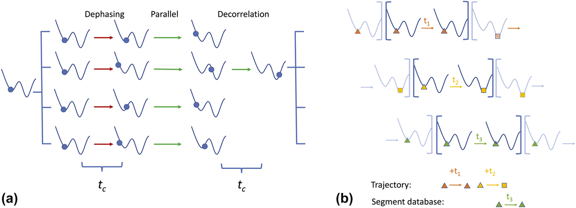
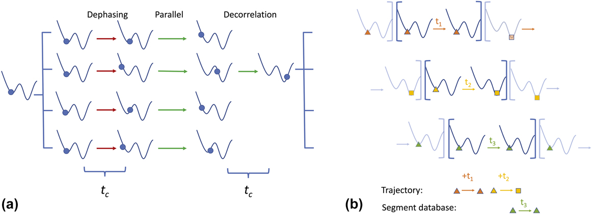
The first method, ParRep, was introduced by Voter in 1998.Reference Voter7 The algorithm proceeds as illustrated in Fig. 2(a). Consider an MD trajectory that is trapped in a given state. One then proceeds to make M − 1 additional copies of the entire system, the replicas. If the number of atoms in the system is sufficient, replicas can internally utilize domain decomposition to further parallelize the calculation of the forces. The first stage of the algorithm, called dephasing, prepares an ensemble of M statistically independent replicas of the system. It does so using a rejection approach: the momenta of the different replicas are randomized and dynamics independently evolved using stochastic thermostats for a time t c. If a system escapes from the initial state before a time t c, it is replaced at its starting position and dephasing is attempted again. At the end of dephasing, the M replicas are located in the same state but are otherwise nominally independent from one another (more on this below). Then begins the parallel stage during which every replica performs MD independently from one another. They, however, periodically check whether a state-to-state transition has occurred. As soon as one is detected, every other replica but the one where the transition has occurred halts its execution. The “winning” replica continues its trajectory for another t c until it settles into a new state; this is the decorrelation stage. This marks the end of a ParRep cycle. The simulation clock is then incremented by the sum of the times accumulated during the parallel and decorrelation stages; the dephasing times do not contribute to the advancement of time.
Schematic illustrations of the two algorithms considered: (a) ParRep and (b) ParSplice. See the text for details.
ParRep is extremely simple but also very accurate. As originally shown by Voter,Reference Voter7 it is exact for Markovian state-to-state dynamics, assuming that configurations separated in time by more than t c without escaping a given state are statistically independent. Recent mathematical analysisReference Le Bris, Lelievre, Luskin and Perez9 has shown that ParRep is even more general: the errors on functions of the state escape times and pathways decrease exponentially with increasing t c, i.e., ParRep can be made arbitrarily accurate for any state definition by simply increasing t c. This is due to the fact that, in the long t c limit, the dephasing stage prepares independent samples from the so-called quasi-stationary distribution (QSD) of a specific state. One can show that starting from the QSD, the next escape process is Markovian, and hence the ParRep procedure is exact. In practice, a finite t c is used, which introduces small errors. However, as the system converges to the QSD exponentially fast, these errors are easy to control: they will be small provided that t c (λ2 − λ1) > 1, where λ2 is the smallest intra-state relaxation rate and λ1 is the quasi-stationary escape rate from the state. Details can be found in the aforementioned publications.Reference Perez, Uberuaga and Voter6,Reference Le Bris, Lelievre, Luskin and Perez9
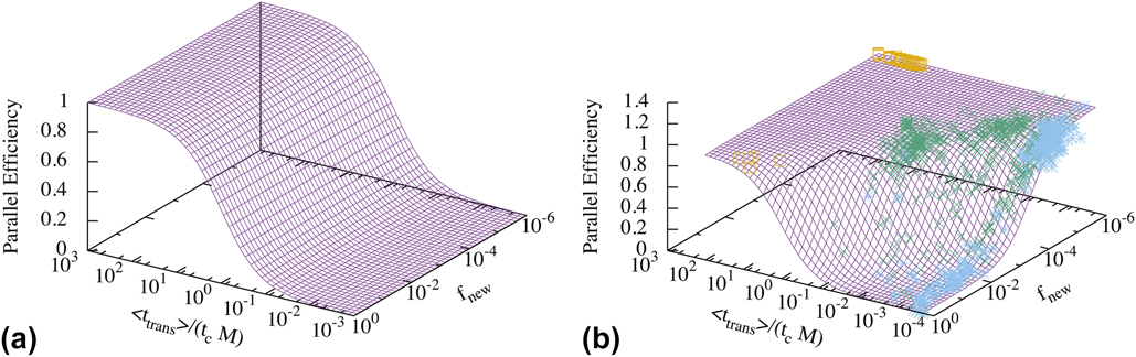
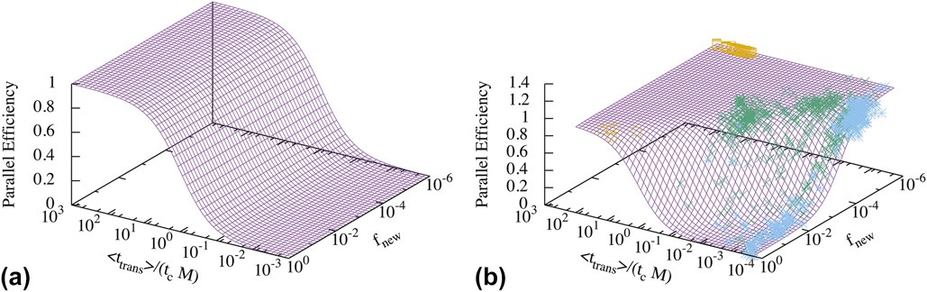
The scalability of ParRep, and by extension the timescales that can be reached, is limited by the overhead introduced by the dephasing step. Taking t trans as a characteristic first escape time in standard serial MD, the ideal parallel speedup is given by t trans/(t c + t trans/M). Thus, the ideal parallel efficiency is given by
 $${{\left[ {{{{t_{{\rm{trans}}}}} / {\left( {{{{t_{\rm{c}}} + {t_{{\rm{trans}}}}} / M}} \right)}}} \right]} / M} = {{{t_{{\rm{trans}}}}} / {\left( {{t_{{\rm{trans}}}} + M{t_{\rm{c}}}} \right)}} = \left( {{{{t_{{\rm{trans}}}}^ * } / {\left( {{t_{{\rm{trans}}}}^ * + 1} \right)}}} \right)\quad ,$$
where t trans* = t trans/(t cM) [see Fig. 3(a)]. Note that this is an upper bound on the actual efficiency as it assumes that dephasing always succeeds, that checking for transitions incurs no computational cost, and that decorrelation and dephasing can be overlapped perfectly (which they often can). This implies that when events are very rare, very large numbers of replicas can efficiently be used. For example, when defining states as energy basins, t c ∼ 1 ps.Reference Perez, Uberuaga and Voter6 So, if transitions occur on ns, μs, or ms timescales, one can leverage 103, 106, or 109 replicas, respectively (which roughly translates to tera, peta, and exascale computers, respectively, when using empirical potentials). ParRep has indeed demonstrated its usefulness at computational scales up to the peta-scale. Examples of use and technical discussion of some practical aspects of ParRep can be found in a recent review.Reference Perez, Uberuaga and Voter6 On the flip side, however, this also means that transitions have to be increasingly rare to exploit even larger machines.
Predicted parallel efficiency of ParRep (a) and ParSplice (b) as a function of the ratio of the first escape time and the total dephasing cost (t cM) and of the probability that the trajectory visits a new state that was never previously encountered, f new. Panel (b) includes actual performance measures during the simulation of the relaxation of disordered Pt nanoparticles: Yellow squares: T = 300 K; green crosses: T = 400 K; blue stars: T = 600 K. The simulation points correspond to averages over 1 wall-clock minute.
What standard ParRep cannot do is leverage larger machines to simulate trajectories with larger numbers of transitions, i.e., to tackle increasingly complex systems where individual transitions are not so rare, but where the interesting behavior only occurs after a very large number of transitions. We recently introduced a new technique, ParSplice,Reference Perez, Cubuk, Waterland, Kaxiras and Voter8 that aims at addressing some of these limitations. ParSplice introduces two new crucial ideas: much can be gained by remembering the past and by predicting the future. Schematically, a ParSplice simulation proceeds as follows [see Fig. 2(b)]. Worker processes [corresponding to different colors in Fig. 2(b)] are individually assigned starting states (represented by the different symbols in the figure). Their task is to generate a so-called trajectory segment that begins in their respective state. These tasks [indicated by square brackets in Fig. 2(b)] are carried out independently on each worker. As soon as the tasks are completed, the worker returns the segments, i.e., the labels of the starting and ending states, as well as the duration of the segments (referred to as t N in the figure), to a dedicated manager process which tries to assemble them (or splice them, in the ParSplice parlance) end-to-end so as to generate a state-to-state trajectory. The rule to do so is very simple: a segment can be spliced at the end of a trajectory as long as its starting state matches the current end state of the trajectory (i.e., as long as the starting and ending symbols match). If a segment cannot immediately be spliced onto the trajectory, it is stored in the segment database for possible reuse; e.g., it can be immediately spliced if the trajectory ever ends up in their starting state at some point in the future. While the manager process does not need complete atomistic states to carry out its work, these are needed by the workers to generate additional segments. Atomistic configurations are therefore stored in a state database that is accessible to all workers. As soon as a worker completes its task, it is assigned a new starting state to generate another segment. As discussed below, these starting states are chosen so as to maximize the probability that the generated segment will be spliced into the main trajectory.
Operationally, a segment is an unbiased section of an MD trajectory such that it is at least t min long (t min is typically ∼1 ps), and that the system did not make a transition for at least t c before the beginning and the end of the segment. Transitions can of course potentially occur within a segment. If a proper starting point (such that the system did spend at least t c in the starting state in the past) is not available, segment generation begins with a dephasing step as in ParRep. Formally, the aim is to generate a section of an MD trajectory whose end points are samples from QSDs. The key concept in ParSplice is that segments so defined can be assembled (spliced) together end-to-end as long as the end and beginning states coincide [i.e., if the symbol shapes match in Fig. 2(b)].
Using the same arguments as in ParRep, one can show this procedure to yield a statistically correct state-to-state trajectory, up to an error that decays exponentially fast in t c.Reference Perez, Cubuk, Waterland, Kaxiras and Voter8 Exploiting this idea in practice requires being able to assess whether a given segment begins in the same state as another one ends. Operationally, this is achieved by labeling states by hashing the connectivity graph of the atoms in the system, following the method introduced in Ref. Reference El-Mellouhi, Mousseau and Lewis10. This bypasses the need to carry out pairwise comparisons between states and allows for the use of lookup tables. Short segments are generated concurrently and the results stored in a database until they are consumed in the trajectory generation.
As the main source of inefficiency in ParRep is dephasing, ParSplice tries to avoid it as much as possible. To do so, ParSplice exploits the fact that the end point of a segment is by construction a valid starting point for the generation of an additional segment that begins in the same state. These samples from the QSD can be reused (albeit only once) whenever more segments are required in an already visited state. This means that, to first order, dephasing only needs to be carried out when a state is visited for the first time; subsequent visits will generate potentially useful segments with little overhead. Coupled with the fact that unused segments are also kept in store for future visits, ParSplice becomes extremely efficient when the trajectory revisits the same states multiple times. The fact that ParSplice can remember previously visited states and exploit the work already done in these is the first innovation compared to ParRep. Although it has been understood that it is possible to increase the efficiency of ParRep by saving the M − 1 nontransitioning trajectory hot points when exiting a state and recalling them when the state is revisited to avoid the dephasing overhead; in fact, most ParRep implementations do not take advantage of this. For this reason, in the present comparison, we will consider the basic ParRep algorithm, which does not exploit this extension.
The second limitation of ParRep is that it is solely focused on the present, as all the replicas are put to work on the current state, even if this could be known to be inefficient (i.e., when t trans < Mt c). It is easy to see that given a prediction of the states that will be visited in the future, it could be more efficient to instead dedicate some of the efforts to working on states that will be visited later. Given a perfect oracle, this approach would be scalable to arbitrary large M. In practice, of course, oracles are not available. ParSplice instead constructs a “statistical oracle”, a Markovian statistical model of the state-to-state evolution over visited states based on previously generated segments. It then uses this model to sample from the optimal distribution of starting states for new segments by minimizing the expected number of times a segment is required to extend the trajectory but is not already available. Operationally, this problem is solved by generating many kinetic Monte Carlo simulations of possible futures of the state-to-state trajectory using the Markovian model and by keeping track of how many additional segments would have been required in each of the known states for ParSplice to create these trajectories. This is carried out on dedicated processes. Starting states are then sequentially selected according to the probability that an additional segment in that state would be used in extending the trajectory. This prediction step in general results in a set of segments that are distributed over several different states, but it always contains some number of segments at the current end state of the trajectory. The details of the procedure can be found in Ref. Reference Perez, Cubuk, Waterland, Kaxiras and Voter8. Exploiting statistical knowledge of possible futures of the trajectory is the second innovation of ParSplice.
To first order, the parallel efficiency of ParSplice at a given moment in its execution can be estimated by
 $$\left( {{{{t_{{\rm{trans}}}}^ * } / {\left( {{t_{{\rm{trans}}}}^ * + {f_{{\rm{new}}}}} \right)}}} \right)\quad ,$$
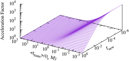
where f new is the probability that the current state has been visited before (in ParRep, this was taken to be 1, as most implementation did not assess whether a state had been visited before). This modification reflects the fact that dephasing only needs to be performed in new states. This expression can, however, underestimate the performance, as it does not account for the fact that previously generated but so far unused segments can be used later, which can lead to effective parallel efficiencies that temporarily exceed 1; we will come back to that point below. It, however, also does not account for the possible need to attempt dephasing more than once, so it is not a true bound on efficiency as in the ParRep case. This expression yields the efficiency surface shown in Fig. 3(b). As shown in the figure, ParSplice fills the performance gap that was left by ParRep when f new is low, independent of the average transition time. In this regime, reuse of past information is maximized, as the trajectory keeps revisiting the same states, and the predictability of the trajectory increases, as a model of the local kinetics quickly becomes accurate due to the frequent revisits. ParSplice can then be significantly more efficient than ParRep, as illustrated in Fig. 4: in the regime where f new is small and transitions are not sufficiently rare to efficiently use the given number M of replicas [t trans/(t cM) is small], ParSplice can be orders of magnitude more efficient that ParRep. It is worth emphasizing again that ParSplice can maintain efficiency even in regimes when individual states are weakly metastable (t trans ∼ t c), so long as these shallow states are organized into super-basins that are themselves sufficiently metastable (so that f new is low). Crucially, this is achieved without having to explicitly define super-basins (which can be a difficult task, especially when it needs to be done on-the-fly); their mere existence entails performance gains.
Performance improvement of ParSplice over ParRep as a function of the ratio of the first escape time and the total dephasing cost (t cM) and of the fraction (or probability) that the trajectory visits a new state that was never previously encountered, f new.
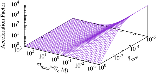
In the opposing limits where individual transitions are very rare [t trans/(t cM) is large] or when states are never revisited (f new = 1), then both ParRep and ParSplice perform essentially the same.
At first sight, it might appear that frequent revisits to the same states might only occur in exceptional situations. In reality, however, it is extremely common. This is rooted in the fact that energy landscapes tend to be structured into the so-called super-basins, i.e., groups of states connected between themselves by low barriers but connected to other super-basins by high(er) barriers. As transition rates are exponentially sensitive to barrier heights, the low-barrier pathways will be selected dramatically more often, especially at low temperatures. Very large numbers of intra-super-basin transitions will, therefore, occur before the trajectory is able to escape, only to be trapped in yet another super-basin. This issue also plagues other long-timescale techniques, like kinetic Monte Carlo.Reference Fichthorn and Lin11–Reference Novotny13 The landscape of large numbers of systems, such as glasses, proteins, nanoclusters, and complex interfaces, is also known to contain large numbers of such super-basins.Reference Wales14 The fact that ParSplice remains extremely efficient in that limit is therefore a very valuable advance.
B. Simulation setup
Simulations of the relaxation of disordered Pt nanoparticles were carried out to validate the performance models. These were performed using the EXAALT framework.15 EXAALT is an open-source software effort supported by the U.S. Department of Energy’s Exascale Computing Project. EXAALT provides an implementation of ParSplice that uses the well-known MD code LAMMPSReference Plimpton16 as a computational engine. Calculations were carried out on the Grizzly system at Los Alamos National Laboratory. Each node contains two 16-core Intel E5 2695v4 Broadwell central processing units (CPUs). Nodes are connected through an Intel OmniPath interconnect.
The system contains 147 Pt atoms interacting through the Voter-Chen embedded atom method (EAM) potential.Reference Voter and Chen17,Reference Voter18 Simulations were initialized from a disordered configuration obtained by abruptly quenching a melted nanoparticle; this structure is therefore initially strongly out of equilibrium. The as-generated disordered nanoparticle possesses an appreciable icosahedral short-range order.Reference Schenk, Holland-Moritz, Simonet, Bellissent and Herlach19,Reference Reichert, Klein, Dosch and Donk20 The relaxation of the disordered state can therefore be expected to relax toward the perfect icosahedron, which is the putative ground state for this number of atoms. While relevant to investigate the relaxation of quenched nanoparticles, the primary motivation behind this choice was to capture widely different dynamical behaviors within a single simulation, and hence to highlight the difference in performance of the two methods in various regimes.
C. Analysis of the evolution of the nanoparticles
As a representative result, we consider a 1.2 ms-long simulation carried out at 600 K. During this period, more than 8 million transitions occurred; these connected 18,271 unique states. To facilitate the analysis of such long trajectories, we clustered the visited states into different groups using the Perron-cluster cluster analysis (PCCA),Reference Deuflhard and Weber21 which has proved very powerful to facilitate the interpretation of long accelerated MD simulations.Reference Huang, Lo, Wen, Voter and Perez22 PCCA defines states as kinetically well-connected sets of states, i.e., super-basins. Using different numbers of clusters provides a way to summarize the behavior of the system over different timescales.
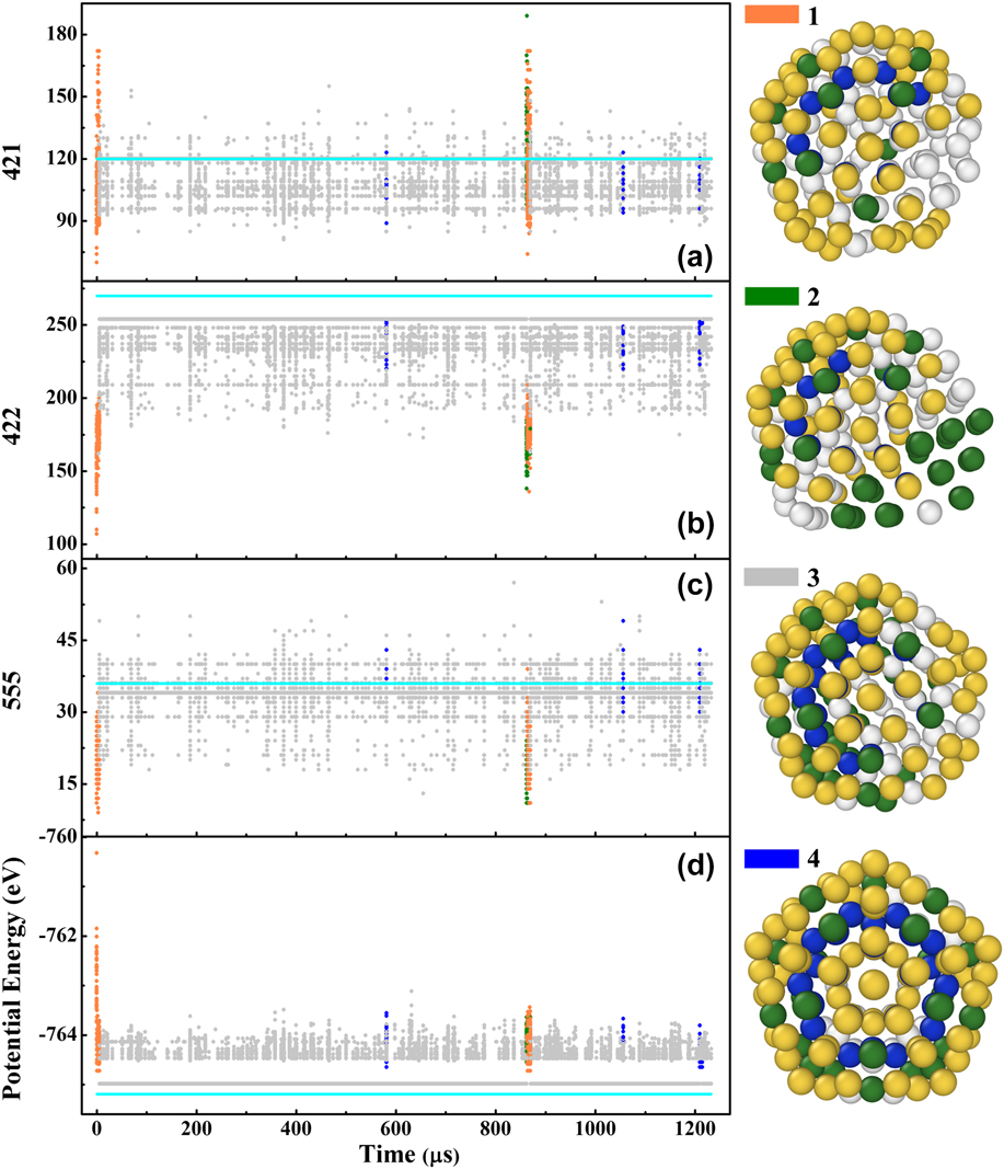
In the following, the number of clusters in the PCCA is set at 4 (see Fig. 5). States in clusters 1 to 4 are, respectively, denoted by orange, green, gray, and blue dots. The structure of these states was characterized using common neighbor analysis (CNA)Reference Clarke and Jónsson23; the reported values are the numbers of different classes of bonds: 421, 422, and 555 bonds are signatures of fcc, hcp, and icosahedral order, respectively. To facilitate comparisons, the corresponding values for the perfect Mackay icosahedron are also indicated by cyan lines.
Left panels: CNA counts and potential energies of all the visited states during a simulation at 600 K. The cyan lines denote the corresponding values for the perfect icosahedron. Right panels: Typical structures of the states in each cluster.

By correlating the CNA values with PCCA clustering, some features of these groups can be highlighted. First, clusters 1 (orange) and 2 (green) contain states with a deficit of 422 and 555 but an excess of 421 bonds relative to the perfect icosahedron. The major difference between these two clusters is that fcc atoms tend to form sizable fcc regions in cluster 2 (green), while they are more dispersed in cluster 1 (orange). Clusters 3 (gray) and 4 (blue) are characterized by CNA counts that are close to those of a perfect icosahedron. Although these two clusters do not show a significant difference in the CNA plots, the central atoms in cluster 4 are found to be in perfect icosahedral order, while those in cluster 1 are not always so (see the corresponding snapshots). Cluster 4 thus has an icosahedral core but exhibits surface defects, mostly “rosette” morphologies that form because the deformation of vertex regions into hexagonal rings allows for an efficient relaxation of the stress on internal atoms.Reference Apra, Baletto, Ferrando and Fortunelli24 Note, however, that PCCA cluster states based on state-to-state kinetics alone; i.e., it does not consider structural similarity between states. Therefore, a simple structural interpretation of the states is not guaranteed; the preceding discussion should only be considered as qualitative and not as a prescription of the features of the states in each cluster. This is reinforced by the considerable overlap between the CNA distribution in each cluster.
As the beginning of the simulation, cluster 1 persists for only a very short time (about 5.6 μs). The system then transitions to cluster 3, whose states tend to exhibit lower energies. Some states in this cluster have energies that are very close to that of the perfect icosahedron [marked by the cyan line in Fig. 5(d)]. This indicates a very fast relaxation of the disordered nanoparticle toward more stable icosahedral configurations. This is consistent with the fact that the free energy barrier between icosahedral and liquid-like states is known to be small in similar small clusters.Reference Doye, Miller and Wales25 During the exploration of this super-basin, the system jumps back to clusters 1 and 2, as well as revisiting cluster 4 once. This shows that even at these moderately elevated temperatures, the structure of the nanoclusters is not static. While icosahedral features remain throughout, the particles can oscillate between states where the structural order differs significantly.
Note that the choice of four PCCA clusters was arbitrary and made mainly for convenience of interpretation. It should not be construed as a statement that only four super-basins exist. For example, Fig. 5 shows that cluster 3 contains a fair amount of internal structure that could be resolved by increasing the number of clusters. The important insight is that the landscape of this system exhibits a hierarchy of super-basins: clusters 1 to 4 individually correspond to super-basins, but their union is also a (super-)super-basin, where the system remains trapped on even longer timescales. Similarly, smaller super-basins almost surely exist.
D. Simulation performance
Benchmark simulations ran for 4 h on 3600 cores, using two threads per core, i.e., M ∼ 7200 worker processes. Note that the 600 K simulation used as a benchmark is a different run than the one analyzed above, as the latter was generated using a different number of cores. The behavior of the different simulations, averaged over whole duration, is summarized in Table I. The results show that, at these scales, simulation rates of ∼1.4 μs/wall-clock minute are possible for this system; this essentially ideal efficiency is achieved at 300 K. As the temperature rises, the simulations are gradually pushed into a regime where the performance of ParRep would be abysmal: except at 300 K, values of t trans* are on the order of 10−3, which implies parallel efficiencies on the same order; i.e., ParRep would essentially run at the same speed as serial MD. At moderate and low temperatures, these trajectories, however, encountered deep super-basins, with average values of f new as low as 2 × 10⁻⁴. As the temperature reaches 800 and 900 K, the super-basins become shallower and f new rises, leading to problems that are essentially out of reach of both ParRep and ParSplice. Two factors contribute to the decrease in performance: (i) some segments are generated but not used (which corresponds to the difference between the generated segment time and the trajectory length) and (ii) higher dephasing costs due to smaller numbers of revisits and multiple dephasing attempts per segment (which is reflected in the decrease of the total generated segment time with increasing temperature).
Performance summary for the ParSplice simulations of the relaxation of disordered Pt nanoparticles at different temperatures. Averages are taken over the entire simulations.

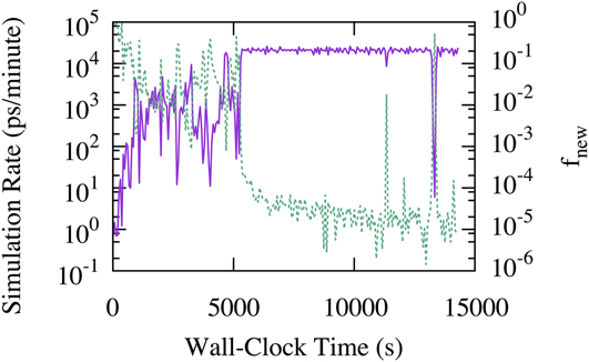
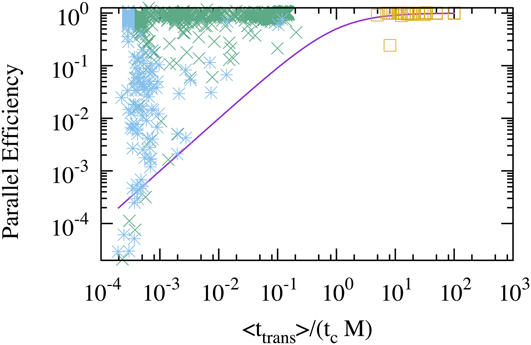
While run-averaged values provide useful overviews of the performance, it is important to realize that performance can significantly vary during a single simulation, especially in this case where the initial configuration is strongly out of equilibrium. For example, as shown in Fig. 6, the simulation rate at 600 K is initially extremely low, as the system quickly relaxes from its initial disordered configuration. During this phase, transitions are extremely rapid and new states are encountered at almost every new transition (f new ∼ 1). After about 1000 wall-clock seconds, the simulation starts to encounter super-basins. These are initially not very deep (f new ∼ 10−2–10−1), but they lead to a significantly increased simulation rate, up to 104–105 ps/min. Finally, after around 5000 s, even deeper super-basins are encountered, leading to a drop in f new below 10−4. This has a dramatic impact on performance, and the simulation rate saturates near its ideal value of around 1.4 μs/min. The same effect can be seen in Fig. 3: during the initial phase of the other simulations, f new was high and t trans* was low, but as the system relaxed, f new gradually decreased. Note that during the whole simulation at 600 K, individual basins themselves did not become deeper: t trans* remained around 10−3 throughout, see Figs. 3 and 7. As shown in Fig. 7, the simulation at 300 K was the only simulation that proceeded in a regime where ParRep would have been efficient; the other ones where orders of magnitude more efficient than what would have been possible with ParRep alone.
Temporal evolution of the efficiency of ParSplice at 600 K. Purple line: simulation rate (left axis); green dashed line: f new (right axis). The simulation data are averaged over 1 wall-clock minute.

Parallel efficiency of ParSplice during the simulation of Pt nanoparticle evolution. Yellow squares: T = 300 K; green crosses: T = 400 K; blue stars: T = 600 K. The continuous purple line is the upper bound on the ParRep efficiency, Eq. (2). The simulation points are averages over 1 wall-clock minute.
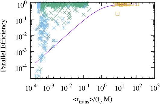
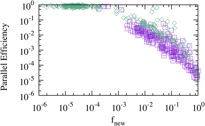
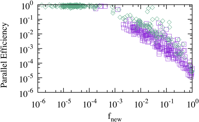
The extensive bookkeeping carried out within ParSplice, i.e., the exploitation of the past visits, is mainly responsible for these performance gains. Indeed, Fig. 3 shows that the simple expression, Eq. (2), correctly captures the actual performance of ParSplice in practice, yet it does not account for the contribution of the predictive model that optimally assigns new segment requests over the known state space. To characterize the benefits of this approach, we carried out another simulation at 600 K where this feature was turned off, i.e., segments were simply requested only at the current end of the trajectory, akin to what is done ParRep. The comparison of the parallel efficiencies is shown in Fig. 8. In both these simulations, t trans* is similar and very small (∼10−4–10−3). The results show that predictions provide a roughly 4× efficiency advantage for f new >10−4; at lower values, the efficiency is essentially 1, so there is no further room for improvement. This can be understood from the fact that very deep super-basins entail large numbers of revisits to the same states. If the total number of segments required in a given state during a visit to a super state is larger than M, then the relative number of leftovers will be small, even if segments are generated M at the time, as in ParRep. For shallower super-states where the number of segments required in a given state is ∼M, then predictions can limit the generation of excess segments by using a finer granularity when requesting additional segments. If the required number drops below M, then all of the segments that are likely to be required to escape will be generated during the first visit to the state, which will typically generate on the order of M segments. The current mode of predictions is therefore not likely to improve the performance as f new tends to 1 and a significant excess of segments will be produced. This behavior can be seen at high temperatures in Table I, where the discrepancy between the trajectory length and the total amount of generated segment time increases.
Measured effect of the predictive segment assignment on performance at 600 K. Green lozenges: ParSplice; purple squares: ParSplice without predictions. The simulation points are averages over 1 wall-clock minute.
III. DISCUSSION
Our benchmarks clearly show that ParSplice excels for systems that contain super-states. In that limit, it can leverage large computing resources to yield extremely long trajectories, even if escapes out of individual states are not rare. It therefore takes an important step toward enabling the investigation of complex systems, where the physics of interest occurs following a very large number of relatively fast unit steps. For example, at 600 K, a 4 h simulation generated a ∼200 μs long trajectory that contained on the order of 90 million transitions or ∼6400 transitions per wall-clock second. This allows for simulations that reach into the milliseconds in less than a day of wall-clock time. In contrast, ParRep would have been limited to around 0.1 transition per second to maintain a similar parallel efficiency.
Challenges, however, remain in the limit where f new is high and t trans* is low. Achieving high performance in this limit will depend almost entirely upon devising more aggressive means to carry out predictions. Indeed, the two main sources of overhead in ParSplice are dephasing and the excess generation of segments. ParSplice reduces the dephasing overhead from once per visit in ParRep to essentially once. This is because on the first visit to a state, it is impossible to predict escapes using only previously seen state-to-state transitions; ParSplice then assumes that no escapes exist, until proven wrong. On the order of M segments will then be executed in every state that is part of the trajectory, except if outgoing transitions were observed before the spliced trajectory reached it. However, if states are shallow and only a few revisits can be expected, generating M segments, each one of them requiring dephasing, is wasteful. What is needed is to predict the number of segments that will be required even before the trajectory reaches a state for the first time. This will require “forward-looking” predictions instead of “backward-looking” ones (i.e., where previous visits to a state are required to make predictions). A range of options to do so are currently being considered, including learning about local rearrangements instead of concentrating on state-to-state transitions and using high-temperature MD to rapidly explore state-space ahead of the advancing trajectory. Note, however, that even with a statistically perfect predictor, the performance of ParSplice will be subject to fundamental limits related to how “predictable” a trajectory is. For example, landscapes that contain a large number of branching points where a trajectory can commit to different regions of configuration space will be inherently hard to predict and will impose limits on the efficiency of ParSplice.
IV. CONCLUSION
Using the evolution of a complex system, initially disordered Pt nanoparticles, we assessed the relative performance of ParRep and ParSplice, two methods for the parallelization of the state-to-state dynamics of systems evolving through sequences of rare events. The analysis demonstrates that ParSplice is especially powerful in the regime where the trajectory is trapped in the so-called super-basins, even when each of the basin-to-basin transitions occurs on a timescale such that the efficiency of ParRep would have been extremely low. In that regime, ParSplice therefore allows for the simulation of very long trajectories that contain extremely large numbers of transitions, allowing for the use of massively parallel resources to investigate the behavior of complex systems. ParSplice is therefore a promising candidate for deployment at the exascale.
ACKNOWLEDGMENTS
This work was supported by the United States Department of Energy (DOE), Office of Basic Energy Sciences, Materials Sciences and Engineering Division (D.P., A.F.V.) and by the China Scholarship Council (R.H.). The development and implementation of the ParSplice code were initially supported by LANL/LDRD Project No. 20150557ER and now by the DOE’s Exascale Computing Project (17-SC-20-SC), a collaborative effort of two U.S. Department of Energy organizations (Office of Science and the National Nuclear Security Administration) responsible for the planning and preparation of a capable exascale ecosystem, including software, applications, hardware, advanced system engineering, and early testbed platforms, in support of the nation’s exascale computing imperative. We gratefully acknowledge computing resources from the Los Alamos Institutional Computing program. Los Alamos National Laboratory is operated by Los Alamos National Security, LLC, for the National Nuclear Security administration of the US DOE under Contract No. DE-AC52-06NA25396.