


1. Introduction
When a fluid layer exists above a horizontal bounding wall, natural convection is triggered when the temperature of the wall is higher than that of the fluid by some extent. Velocity and temperature boundary layers are formed over the bounding wall beyond some value of the temperature difference (Gill, Zeh & Casal Reference Gill, Zeh and Casal1965; Rotem & Claassen Reference Rotem and Claassen1969; Pera & Gebhart Reference Pera and Gebhart1973). These boundary layer flows are driven by the horizontal pressure gradient induced by the presence of denser fluid outside the boundary layer and lighter fluid inside it (Stewartson Reference Stewartson1958; Gebhart et al. Reference Gebhart, Jaluria, Mahajan and Sammakia1988). Studies, both experimental (Clausing & Berton Reference Clausing and Berton1989; Kitamura & Kimura Reference Kitamura and Kimura1995; Radziemska & Lewandowski Reference Radziemska and Lewandowski2001; Kozanoglu & Lopez Reference Kozanoglu and Lopez2007) and theoretical (Merkin Reference Merkin1985; Chen, Tien & Armaly Reference Chen, Tien and Armaly1986; Umemura & Law Reference Umemura and Law1990; Samanta & Guha Reference Samanta and Guha2012), abound on such natural convection boundary layers due to their presence in a large number of applications. Equivalent phenomena, often at high Schmidt numbers  $Sc = \nu /D$, where
 $\nu$ is the kinematic viscosity and
 $D$ is the molecular diffusivity of the species in the fluid, occur when the concentration of a species on the wall is lesser than that in the fluid (Goldstein, Sparrow & Jones Reference Goldstein, Sparrow and Jones1973; Lloyd & Moran Reference Lloyd and Moran1974). In such cases, the relative thicknesses of the velocity and concentration boundary layers depend on the value of
 $Sc$.
When such boundary layers form over horizontal porous surfaces that have a normal flow of lighter fluid through them, which we hereinafter refer to as blowing, the density distribution and hence the driving pressure gradient within the boundary layers change from the case of that in natural convection boundary layers (NBL). Blowing then modifies the velocities within these boundary layers, and the dependence of the boundary layer thicknesses on the horizontal coordinate,  $x$. These changes in turn drastically alter the instability of the boundary layers, leading to changes in the distribution of flow structures and the transport of species across the boundary layers. Understanding such boundary layers is important since they abound in industrial processes such as catalysis (Shemilt & Sedahmed Reference Shemilt and Sedahmed1976), separation by membranes (Tanaka Reference Tanaka1991; Slezak et al. Reference Slezak, Grzegorczyn, Jasik-Slezak and Michalska-Malecka2010), ultrafiltration (Youm, Fane & Wiley Reference Youm, Fane and Wiley1996), carbon sequestration (Kneafsey & Pruess Reference Kneafsey and Pruess2010; Huppert & Neufeld Reference Huppert and Neufeld2014), membrane fabrication (Atkinson & Lloyd Reference Atkinson and Lloyd2000), drying (Coussot Reference Coussot2000) and burning of fuel films (Clarke & Riley Reference Clarke and Riley1976).
The governing equations for these boundary layers allow similarity solutions only for practically difficult experimental configurations, namely, for a  $x^{-2/5}$ dependence of the blowing velocity
 $V_i$ (Clarke & Riley Reference Clarke and Riley1975; Merkin Reference Merkin1975; Lin & Yu Reference Lin and Yu1988; Chen, Buchanan & Armaly Reference Chen, Buchanan and Armaly1993). For the more practical, and often encountered, case of a spatially uniform blowing velocity
 $V_i$, Chen et al. (Reference Chen, Buchanan and Armaly1993) obtained numerical solutions for various values of their non-similarity parameter
 $\xi _1=5^{1/5} Re_x/Gr_x^{1/5}$. Here,
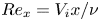 $Re_x=V_i x/\nu$ is the Reynolds number based on
 $V_i$ and
 $x$ while
 $Gr_x=g\beta {\rm \Delta} C x^3/\nu ^2$ is the Grashof number based on the driving concentration potential
 ${\rm \Delta} C$ and
 $x$, with
 $g$ being the gravitational acceleration and
 $\beta$ the coefficient of salinity. These results are however limited to a low Prandtl number of
 $Pr=0.7$, which would occur in temperature driven convection in gases; they also did not obtain closed-form scaling laws for the boundary layer thicknesses and the velocity distributions. The case of a spatially constant
 $V_i$ for these boundary layers were also obtained by Puthenveettil & Arakeri (Reference Puthenveettil and Arakeri2004), however again only at a low
 $Pr = 1$ (or
 $Sc = 1$), by numerical solutions of integral equations; the study did not give rise to any understanding of the scaling of these boundary layers.
Unlike in the above cases, the most common occurrences of these boundary layer flows are in liquid systems where the convection is driven by concentration differences, often with a spatially constant blowing velocity (see Shemilt & Sedahmed Reference Shemilt and Sedahmed1976; Tanaka Reference Tanaka1991; Youm et al. Reference Youm, Fane and Wiley1996). Since the molecular diffusivity of solutes are low, such systems have high  $Sc({\sim }10^3)$, resulting in the formation of very thin species boundary layers over the horizontal porous surface. The present study considers such high
 $Sc$ natural convection boundary layers forming over a horizontal permeable surface which are subjected to a weak constant blowing velocity
 $V_i$ through the membrane. When such boundary layers at high
 $Sc$ are subjected to transpiration, even a weak blowing would ensure uniform concentration, equal to the concentration of the transpiring fluid, within the thin species boundary layer. For such boundary layers, we present a theoretical analysis which proposes scaling laws for the boundary layer thicknesses, the horizontal velocity and the drag.
We create these boundary layers experimentally on the surface of a horizontal micro porous membrane by arranging a layer of brine over a layer of water across the membrane and gravitationally forcing a steady and uniform stream of water through the membrane from below. Thin, high  $Sc$, natural convection boundary layers form at several spatially and temporally random locations on the membrane surface (Puthenveettil & Arakeri Reference Puthenveettil and Arakeri2005, Reference Puthenveettil and Arakeri2008; Ramareddy & Puthenveettil Reference Ramareddy and Puthenveettil2011). These boundary layers are naturally unstable due to the unstable density gradients across them, resulting in them rising upward in the form of line plumes, after some longitudinal distance of travel. The rising plumes become turbulent after a short distance, resulting in turbulent ambient and diffusive boundary layers on the membrane turning into rising plumes. We choose one of such boundary layers that occur in our experiments, before their instability, and conduct an integral analysis of their governing equations under the approximation that most of the species boundary layer contains a uniform concentration of
 $C_B$.
The analysis is conducted at large Grashof numbers,  $Gr_L=g\beta {\rm \Delta} C L^3/\nu ^2({\sim }10^4)$, for weak blowing (
 $V_i \leq 0.1$ mm s
 $^{-1}$) with no appreciable diffusion effects (
 $V_i \geq 0.01$ mm s
 $^{-1}$) in the species boundary layer, where
 $L$ is the length of the boundary layer; the corresponding range of Reynolds number of blowing is
 $0.112 \leq Re_L = V_iL/\nu \leq 1.12$. Though there exists a blowing velocity
 $V_i$ into the boundary layers, since
 $10^{5} < Gr_L/Re_L^{5/2} < 10^7$, natural convection effects dominate over the shear effects due to blowing. We observe similarity of the boundary layer thicknesses and the velocity profile for such a regime; the similarity allows us to propose simple relations for these quantities. We then obtain an expression for the horizontally averaged concentration profile in the species boundary layer using these relations, which surprisingly, is seen to be independent of
 $V_i$. Such a theoretical average concentration profile, as well as the species boundary layer thicknesses, are then shown to match with those obtained from the planar laser-induced fluorescence (PLIF) images obtained in our experiments, thereby verifying these theoretical relations.
The paper is organised as follows. In § 2.1 we formulate the integral boundary layer equations, which are then simplified using the uniform concentration approximation discussed in appendix A; the relevant characteristic scales are discussed in appendix B. In § 2.2 these scales are used to normalise the integral equations to arrive at their dimensionless form. The theoretical variations of the species boundary layer thickness  $\delta _d(x)$, the horizontal velocity profiles
 $u(x,y)$ and the velocity boundary layer thickness
 $\delta _v(x)$ along with the wall shear stress are discussed in §§ 3.1, 3.2 and 3.3, respectively; these sections also give the associated dimensionless relations for these variables. The details of the theoretical mean concentration profile are given in § 3.4. The experimental set-up and diagnostics are discussed in §§ 4.1 and 4.2, respectively. The theoretical and the experimental mean concentration profiles are compared in § 5, before concluding in § 6.
2. Integral formulation
2.1. Integral boundary layer equations
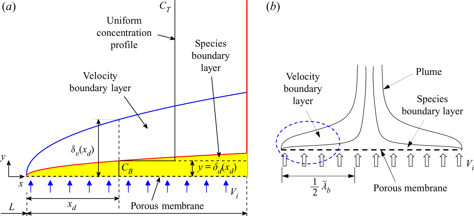
Consider a steady, laminar, incompressible, natural convection boundary layer over a horizontal porous surface with an upward vertical normal flow velocity ( $V_i$) through the surface as depicted in figure 1(a). The equations governing such a boundary layer are
 \begin{gather} \frac{\partial u}{\partial x} + \frac{\partial v}{\partial y}=0, \end{gather}
 \begin{gather}u\frac{\partial u}{\partial x} + v\frac{\partial u}{\partial y} = -\frac{1}{\rho} \frac{\partial p_{m}}{\partial x} + \nu \frac{\partial ^{2} u} {\partial y^{2}}, \end{gather}
 \begin{gather}\frac{1}{\rho}\frac{\partial p_{m}}{\partial y}=g\beta (C_{T}-C), \end{gather}
 \begin{gather}u\frac{\partial C}{\partial x} + v\frac{\partial C}{\partial y} = D\frac{\partial ^{2} C}{\partial y^{2}}, \end{gather}
where  $u$ and
 $v$ are the components of velocity in the
 $x$ and
 $y$ directions,
 $p_{m}(x,y)=p-p_s$ is the motion pressure,
 $p$ is the actual local pressure and
 $p_s$ is the local hydrostatic pressure when the fluid density is everywhere at
 $\rho$, the ambient density above the boundary layer. The concentration of species within the species boundary layer is
 $C(x,y)$ and the concentration of the species above the species boundary layer is
 $C_T$. The boundary conditions for the wall-blowing case are
 \begin{gather} \mathrm{at}\ y = 0: u = 0; \quad v = V_i; \quad C = C_{B},\quad \textrm{and} \end{gather}
 \begin{gather}\mathrm{at}\ y = \delta_{v}: u = 0;\quad \frac{\partial u}{\partial y} = 0;\quad v = V_{\delta_{v}}; \quad C = C_{T};\quad \frac{\partial C}{\partial y} = 0, \end{gather}
where  $C_B$ is the concentration of the species on the membrane and
 $V_{\delta _{v}}$ is the vertical velocity at the edge of the velocity boundary layer. In (2.6a–e),
 $\partial u/\partial y |_{y=\delta _v} = 0$ is obtained by applying (2.2) at
 $y=\delta _v$, since
 $p_m = 0$ for all
 $y\geq \delta _v$, implying that
 $\partial p_m/\partial x |_{y=\delta _v} = 0$,
 $u |_{y=\delta _v} = 0$, and neglecting the viscous resistance at
 $y=\delta _v$.
(a) Schematic of a laminar natural convection boundary layer on a horizontal porous surface with a uniform normal blowing through the surface. The assumed uniform concentration profile between the ambient concentration  $C_T$ and the surface concentration
 $C_B$ is shown at
 $x=x_d$. (b) Schematic of a plume that results from the instability of a pair of such boundary layers. Here
 $\bar {\lambda }_b$ (3.15) is the mean distance between the edges of the adjacent plumes (Puthenveettil & Arakeri Reference Puthenveettil and Arakeri2008). The zoomed view of the region in the dotted ellipse is shown in (a).

By integrating (2.2) from the membrane surface to  $\delta _v(x)$, we obtain
 \begin{equation} \frac{1}{2}\frac{\mathrm{d}}{\mathrm{d}x}\int_0^{\delta_v}u^2\,\textrm{d} y+ \int_0^{\delta_v}v\frac{\partial u}{\partial y}\textrm{d} y+ \frac{1}{\rho}\int_0^{\delta_v}\frac{\partial p_m}{\partial x}\textrm{d} y+ \nu \left. \frac{\partial u}{\partial y}\right |_{y=0}=0. \end{equation}
Expanding the second term in (2.7) as  $\int _0^{\delta _v} (\partial (uv)/\partial y-u \partial v/\partial y)$, replacing
 $\partial v/\partial y$ with
 $-\partial u/\partial x$ from (2.1) and using the boundary condition for
 $u$ from (2.5a–c) and (2.6a–e), we obtain
 \begin{equation} \int_0^{\delta_v}v\frac{\partial u}{\partial y}\textrm{d} y = \int_0^{\delta_v}u\frac{\partial u}{\partial x}\textrm{d} y. \end{equation}
Utilizing (2.8) in (2.7) and simplifying, we obtain the integral  $x$-momentum equation as
 \begin{equation} \frac{\mathrm{d}}{\mathrm{d}x}\int_0^{\delta_v}u^2\,\textrm{d} y+ \frac{1}{\rho}\int_0^{\delta_v}\frac{\partial p_m}{\partial x}\textrm{d} y+\nu \left. \frac{\partial u}{\partial y}\right |_{y=0}=0. \end{equation}
Equation (2.9) expresses a balance between the driving force due to the motion pressure gradient, the viscous resistance and the inertial forces.
Integrating (2.4) from  $y=0$ to
 $\delta _d(x)$, after replacing
 $v\partial C/\partial y$ with
 $\partial (vC)/\partial y-C\partial v/\partial y$, and simplifying using
 $v |_{y=\delta _d} = V_{\delta _d}$,
 $C |_{y=\delta _d} = C_T$,
 $v |_{y=0} = V_i$ and
 $C |_{y=0} = C_B$, we get
 \begin{equation} \int_0^{\delta_d}u\frac{\partial C}{\partial x}\textrm{d} y + V_{\delta_d}C_T - V_iC_B - \int_0^{\delta_d}C\frac{\partial v}{\partial y}\textrm{d} y = -D\left. \frac{\partial C}{\partial y}\right |_{y=0}. \end{equation}
In arriving at (2.10), we used  $\partial C/\partial y |_{y=\delta _d} = 0$, obtained by applying (2.4) at
 $y=\delta _d$ since diffusion and
 $\partial C/\partial x$ are negligible at
 $y=\delta _d$. Replacing
 $\partial v/\partial y$ in (2.10) with
 $-\partial u/\partial x$ from (2.1) and since
 $u\partial C/\partial x = \partial (uC)/\partial x - C\partial u/\partial x$, (2.10) simplifies to
 \begin{equation} \int_0^{\delta_d}\frac{\partial}{\partial x}(uC)\,\textrm{d} y + V_{\delta_d}C_T - V_iC_B + D \left. \frac{\partial C}{\partial y}\right |_{y=0} = 0. \end{equation}
Expanding the first term in (2.11) using Leibnitz rule, we obtain (2.11) as
 \begin{equation} \frac{\mathrm{d}}{\mathrm{d}x}\int_0^{\delta_d}(uC)\,\textrm{d} y - C_T\left. u\right |_{y=\delta_d} \frac{\mathrm{d} \delta_d}{\mathrm{d}x} + V_{\delta_d}C_T -V_iC_B +D\left. \frac{\partial C}{\partial y}\right |_{y = 0} = 0. \end{equation}
An expression for  $V_{\delta _d}$ in (2.12) can be obtained by integrating (2.1) from
 $y=0$ to
 $\delta _d(x)$ to get
 \begin{equation} \frac{\mathrm{d}}{\mathrm{d}x}\int_0^{\delta_d}u\,\textrm{d} y -\left. u\right |_{y=\delta_d} \frac{\mathrm{d}\delta_d}{\mathrm{d}x} + V_{\delta_d}-V_i=0. \end{equation}
Now, replacing the second and third terms in (2.12) with  $C_TV_i - C_T\,\mathrm {d}/\mathrm {d}x(\int _0^{\delta _d}u\,\textrm {d} y)$, obtained by multiplying (2.13) with
 $C_T$, we obtain the integral species conservation equation as
 \begin{equation} \frac{\mathrm{d}}{\mathrm{d}x}\int_{0}^{\delta_{d}} u(C-C_{T})\,\textrm{d} y + V_{i} {\rm \Delta} C +D\left. \frac{\partial C}{\partial y}\right |_{y = 0} = 0, \end{equation}
where  ${\rm \Delta} C=C_T-C_B$.
2.1.1. Reduced integral equations using uniform concentration approximation
In high  $Sc$ natural convection boundary layers, as the diffusivity of momentum would be much larger than that of the species, the species boundary layer would be much thinner than the velocity boundary layer. A weak wall-normal flow would hence produce a uniform concentration in most of the species boundary layer region. The concentration in the species boundary layer could then be approximated to be uniform and equal to the concentration at the surface of the membrane
 $C_{B}$ and, thus, within the species boundary layer,
 \begin{equation} C_{T}-C\simeq C_{T} - C_{B} = {\rm \Delta} C. \end{equation}
Such a uniform concentration approximation is valid only above a lower limit of the blowing velocity, below which appreciable diffusive effects will be present to cause a non-negligible concentration drop across the species boundary layer. We show in appendix A that the approximation (2.15) is valid for  $V_i\ge 0.001$ cm s
 ${^{-1}}$, or in terms of the dimensionless blowing parameter, defined in (2.21),
 $B\ge 0.012$. The corresponding upper limit of the present analysis,
 $V_i\le 0.01$ cm s
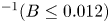 $^{-1} (B\le 0.012)$ is obtained in § 3 so that the inertial effects are negligible within the boundary layers.
Integrating the  $y$-momentum equation (2.3) with respect to
 $y$, using the condition
 ${p_{m}}_{|y=\delta _d} = 0$, and since
 $\int _0^{\delta _d}(C_T-C)\,\textrm {d} y = {\rm \Delta} C\delta _d$ by the uniform concentration approximation (2.15), we obtain
 \begin{equation} p_{m} = -\rho g\beta {\rm \Delta} C(\delta_{d}-y) \end{equation}
as the motion pressure distribution in the species boundary layer. Substituting (2.16) in the second term in (2.9) and applying Leibnitz rule to write the term as  $\partial /\partial x\int _0^{\delta _d}(\delta _d-y)\,\textrm {d} y$ results in the integral momentum equation for high
 $Sc$ NBL on a horizontal porous surface with blowing, subject to the uniform concentration approximation (2.15),
 \begin{equation} \frac{\mathrm{d}}{\mathrm{d}x}\int_{0}^{\delta_{v}} u^{2}\,\textrm{d} y - \frac{1}{2}g\beta{\rm \Delta} C\frac{\mathrm{d}\delta_d^2}{\mathrm{d}x} + \nu \left. \frac{\partial u}{\partial y}\right |_{y=0} = 0. \end{equation}
In arriving at (2.17), the upper limit of the integral of the pressure gradient term in (2.9) was changed to  $\delta _d$, as
 $p_m = 0$ for
 $y\geq \delta _v$. The integral species (2.14), under the uniform concentration approximation (2.15), reduces to
 \begin{equation} \frac{\mathrm{d}}{\mathrm{d}x}\int_{0}^{\delta_{d}} u\,\textrm{d} y = V_i. \end{equation}
2.2. Dimensionless integral equations
Normalizing the terms in (2.17) with the corresponding characteristic scales, obtained in appendix B, we get the dimensionless integral momentum equation as
 \begin{equation} Sc^{2/5}B^{5/4}\hat{\delta}_v(\hat{\delta}_vI_{M})^{\prime}-Sc^{1/5} \hat{\delta}_v\hat{\delta}_d\hat{\delta}_d^{\prime}+\left. \frac{\partial \hat{u}(\hat{x},\eta)}{\partial \eta}\right |_{\eta=0}=0. \end{equation}
Here,  $\hat {x}=x/L$,
 $\hat {\delta }_d=\delta _d/\delta _{dc}$,
 $\hat {\delta }_v =\delta _v/\delta _{vc}$,
 $\hat {u}=u/u_c$, with all the
 $\hat {}$ variables hereinafter indicating such normalised terms and
 ${}^{\prime }$ denoting differentiation with respect to
 $\hat {x}$. Here
 $I_{M} = \int _{0}^{1} {\hat {u}(\hat {x},\eta )}^2\,\textrm {d}\eta$ and
 $\eta = y/\delta _v$ is the dimensionless vertical coordinate. The characteristic scales
 $\delta _{dc}$,
 $u_c$ and
 $\delta _{vc}$ are given by (B 5), (B 6) and (B 7), respectively, in appendix B. Since the characteristic scales (B 5) and (B 6) were obtained under the condition that
 \begin{equation} Re_{\delta_v}=\frac{V_i \delta_{vc}}{\nu}\ll 1 \end{equation}
the specific form of (2.19) is applicable only when (2.20) is satisfied. Note that in (2.19), the dimensionless blowing parameter,
 \begin{equation} B = \frac{Re_L}{Gr_L^{1/5}}, \end{equation}
that characterises the strength of blowing compared to the buoyancy and the viscous effects, appears as the relevant dimensionless number, on which the dimensionless boundary layer thicknesses and horizontal velocity depend.
Normalizing (2.18) with the characteristic scales, we get the dimensionless integral species equation as
 \begin{equation} (\hat{\delta}_{d} I_{S})^{\prime} = 1, \end{equation}
where  $I_{S} = \int _{0}^{1} {\hat {u}(\hat {x},\eta )}\,\textrm {d}\eta _{d}$, with
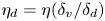 $\eta _{d} = \eta (\delta _v/\delta _d)$. The dimensionless boundary conditions obtained from (2.5a–c) and (2.6a–e) are
 \begin{gather} \textrm{at}\ \eta = 0: \hat{u} = 0; \quad \hat{v} = 1; \quad \hat{C}_B = \frac{C_B}{{\rm \Delta} C},\quad\mathrm{and} \end{gather}
 \begin{gather}\textrm{at}\ \eta = 1: \hat{u} = 0; \quad \frac{\partial \hat{u}(\hat{x},\eta)}{\partial \eta} = 0; \quad \hat{v} = \frac{V_{\delta_{v}}}{V_i}; \quad \hat{C}_T = \frac{C_T}{{\rm \Delta} C}, \end{gather}
where  $\hat {v}=v/V_i$.
Since (2.19) and (2.22) can be solved for  $\hat {\delta }_v$ and
 $\hat {\delta }_d$ only when
 $\hat {u}(\hat {x},\eta )$ is known, we approximate the dimensionless horizontal velocity distribution as
 \begin{equation} \hat{u}(\hat{x},\eta)=K_{1}+ K_{2}\eta + K_{3}\eta^{2} + K_{4}\eta^{3}. \end{equation}
The expressions for  $K_{1}$ to
 $K_{4}$, given in appendix C, are obtained by using the boundary conditions for
 $\hat {u}$ and
 $\partial \hat {u}/\partial \eta$ in (2.23a–c) and (2.24a–d), along with the dimensionless
 $x$-momentum equation at the wall,
 \begin{equation} Sc^{1/5}B^{5/4}\hat{\delta}_v\left. \frac{\partial \hat{u}(\hat{x},\eta)}{\partial \eta}\right |_{\eta =0} -Sc^{2/5}\hat{\delta}_v^2\,\hat{\delta}_d^{\prime}-\left. \frac{\partial ^{2}\hat{u}(\hat{x},\eta)}{\partial \eta^{2}}\right |_{\eta =0} = 0. \end{equation}
Substituting the expressions for  $K_{1}$ to
 $K_{4}$ from (C 1) to (C 4) in (2.25) and simplifying, (2.25) can be written as
 \begin{equation} \hat{u}(\hat{x},\eta) = \frac{\eta(\eta - 1)^{2}\hat{\delta}_v^2 \hat{\delta}_d'Sc^{2/5}}{4 + B^{5/4}Sc^{1/5}\hat{\delta}_v}. \end{equation}
Substituting (2.27) in (2.19) and (2.22) we obtain two dimensionless, second-order nonlinear ordinary differential equations,
 \begin{gather} E_1(\hat{\delta}_d^{\prime})^2\hat{\delta}_v^{\prime}+E_2 \hat{\delta}_d^{\prime}+E_3\hat{\delta}_d^{\prime}\hat{\delta}_d^{\prime \prime} = 0 \quad \textrm{and} \end{gather}
 \begin{gather}E_{4}(\hat{\delta}_d^{\prime})^2+E_{5}\hat{\delta}_d^{\prime} \hat{\delta}_v^{\prime}+E_6\hat{\delta}_d^{\prime \prime}-1=0, \end{gather}
where  $^{\prime \prime }$ denotes double differentiation with respect to
 $\hat {x}$ and the expressions for the coefficients
 $E_1$ to
 $E_6$, that are functions of
 $\hat {\delta}_v, \hat {\delta}_d$ and
 $B$, are given in appendix C.
3. Theoretical profiles
We numerically solve (2.28) and (2.29) to obtain  $\hat {\delta}_v$ and
 $\hat {\delta}_d$ as functions of
 $\hat {x}$ for
 $0.012\leq B \leq 0.12$ at
 $Sc=600$ (see table 1). As discussed in appendix A, the above lower limit of
 $B$ is chosen so that diffusive effects are not appreciable in the species boundary layer, due to which the uniform concentration approximation (2.15) can be applied. The above upper limit of
 $B$ is chosen so as to satisfy (2.20). This upper limit of the analysis, also defines the upper limit of ‘weak’ blowing so that the inertial effects are negligible. The range of
 $V_i$ (0.001–0.01 cm s
 $^{-1}$) specified in table 1, corresponding to the above range of
 $B$, corresponds to the specific
 ${\rm \Delta} C$,
 $L$ and fluid properties specified in table 2.


The physical situation envisaged is that of a fixed  $Gr_L=8.69\times 10^4$ for a brine layer of 10 gl
 $^{-1}$ concentration above a horizontal porous surface, through which a weak upward normal flow with a Reynolds number range of
 $0.112\leq Re_L\leq 1.12$, corresponding to a changing
 $V_i$, occurs into the layer. The dimensionless solutions are however valid for other physical situations that satisfy
 $0.012\leq B\leq 0.12$ and
 $Sc \gg 1$. The conditions at the leading edge used to initiate the dimensionless solutions are
 $\hat {\delta}_v = \hat {\delta}_d = 0.018$ and
 ${\hat {\delta}_d}^{\prime }= 6369.7$, calculated from the similarity solutions of Rotem & Claassen (Reference Rotem and Claassen1969) for the corresponding no blowing case at
 $\hat {x}$ =
 $10^{-6}$. The characteristic scales needed to convert these dimensionless solutions to the needed dimensional values are also calculated using the parameters shown in table 2.
3.1. Species boundary layer thickness
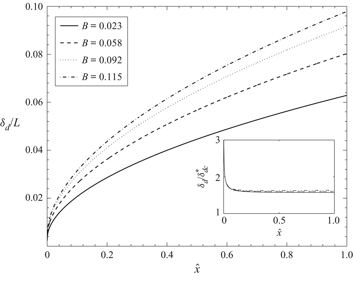
Figure 2 shows the variation of the dimensionless species boundary layer thickness  $\delta _{d}/L$ with the dimensionless horizontal position
 $\hat {x}$ for different blowing parameters
 $B$. Blowing more lighter fluid into the species boundary layer results in a larger thickness of the boundary layer as well as a larger slope of the boundary layer edge at any
 $\hat {x}$, the reason for which could be the following. Equation (2.18) implies that the additional lighter fluid in the species boundary layer increases the horizontal momentum flux in the species boundary layer which increases the inertial forces in the boundary layer as per (2.17). This increase in inertial forces is then balanced by a corresponding net increase in the motion pressure gradient and the wall shear stress. The integral of the motion pressure gradient is proportional to
 $\delta _d\,\mathrm {d}\delta _d/\mathrm {d}x$, as inferred from (2.16) and the second term in (2.17). With blowing, in addition to the increase of the viscous shear stress, it appears that a simultaneous increase of
 $\delta _d$ and
 $\textrm {d}\delta _d/\textrm {d} x$ is necessary to balance the increased inertial forces in the boundary layer; blowing then increases the species boundary layer thickness and its longitudinal gradient.
Variation of the dimensionless species boundary layer thickness with the dimensionless horizontal position for various blowing parameter values. The inset shows that  $\delta _{d}/{\delta }_{dc}^{*}$, where
 ${\delta }_{dc}^{*}$ is given by (3.1), is independent of
 $B$ and
 $\hat {x}$ except very close to the leading edge.

The inset of figure 2 shows the dependence of  $\delta _{d}/{\delta }_{dc}^{*}$ on
 $\hat {x}$ for different blowing parameters, where
 \begin{equation} {\delta}_{dc}^{*} = \left(\frac{\nu V_{i} x^{2}}{g\beta{\rm \Delta} C}\right)^{1/4} \end{equation}
is obtained by replacing  $L$ in (B 5) with
 $x$. The figure shows that
 $\delta _{d}/{\delta }_{dc}^{*} \simeq 1.6$, which implies that, contrary to the earlier observations (Chen et al. Reference Chen, Buchanan and Armaly1993; Puthenveettil & Arakeri Reference Puthenveettil and Arakeri2004) of the non-similar nature of these boundary layers, for the present range of
 $B$, at high
 $Sc$, these boundary layers do show a similar nature. The species boundary layer thickness is then given by
 \begin{equation} \frac{\delta_{d}}{x} \simeq 1.6 \left(\frac{\nu V_i}{g\beta {\rm \Delta} Cx^2}\right)^{1/4} = 1.6 \left(\frac{Re_{x}}{Gr_{x}}\right)^{1/4}=1.6\frac{B^{5/4}}{Re_L}\sqrt{\frac{L}{x}}. \end{equation}
The scaling (3.2), captures the increase of  $\delta _d$ and
 $\mathrm {d}\delta _d/\mathrm {d}x$ with
 $V_i$ at any
 $x$, seen in figure 2. The physical explanation for such scaling, as is clear from (3.1), is that the order of magnitude balance in (B 3) at a distance of
 $L$, which reduces to balance of motion pressure gradient and viscous resistance at
 $Re_{\delta _v}\ll 1$, also becomes valid at each
 $x$ to give rise to (3.2). It also implies that since
 $\delta _d/\delta _{dc}^{*}$ is of order one,
 $\delta _{dc}$ is the appropriate characteristic scale for
 $\delta _d$, implying that
 $\delta _d$ has a square root dependence on
 $x$ and a one-fourth power law dependence on
 $V_i$ for a given fluid and concentration difference.
The scaling (3.2) can also be written in terms of the length scales near the porous surface as
 \begin{equation} \frac{\delta_{d}}{x} \simeq 1.6\left(\frac{Z_w^3Sc}{Z_{V_i}x^2}\right)^{1/4}, \end{equation}
where
 \begin{equation} Z_w =\left(\frac{\nu D}{g\beta {\rm \Delta} C}\right)^{1/3}\quad \mathrm{and}\quad Z_{V_i} = \frac{\nu}{V_i} \end{equation}
are the near-wall length scales in turbulent convection obtained due to a balance of diffusive and buoyancy forces (Theerthan & Arakeri Reference Theerthan and Arakeri1998; Puthenveettil et al. Reference Puthenveettil, Gunasegarane, Agrawal, Schmeling, Bosbach and Arakeri2011) and the advective-viscous length scale (Puthenveettil & Arakeri Reference Puthenveettil and Arakeri2008), respectively.
3.2. Velocity profiles
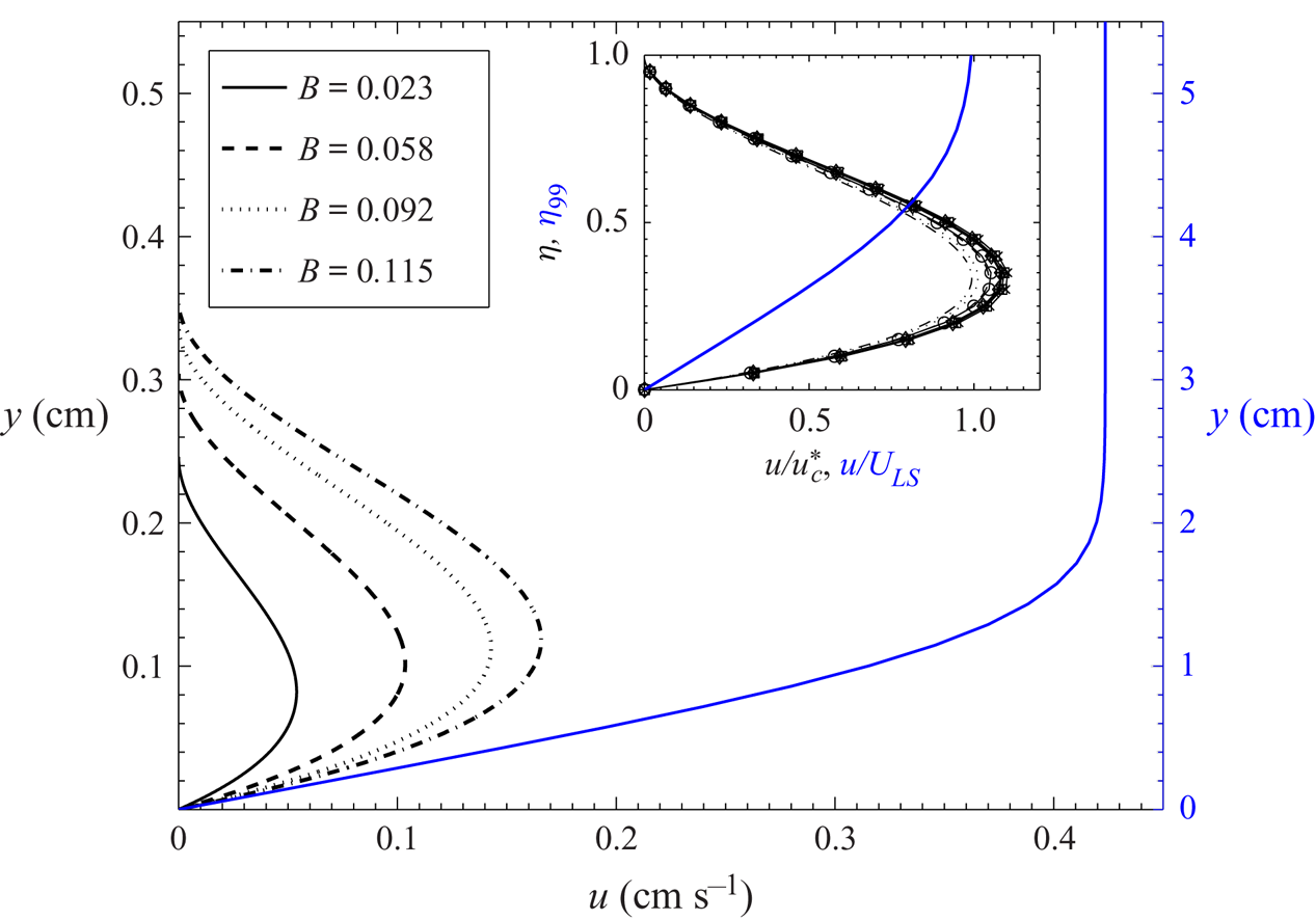
Figure 3 shows the effect of blowing on the horizontal velocity profiles in the boundary layer at  $\hat {x}=1.0$. Here,
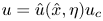 $u = \hat {u}(\hat {x},\eta )u_c$, where
 $u_c$ is given by (B 6), and
 $\hat {u}(\hat {x},\eta )$ is determined by substituting
 $\hat {\delta}_v$,
 $\hat {\delta}_d$ and
 $\hat {\delta}_d'$, obtained from the solution of (2.28) and (2.29), in (2.27). As discussed earlier, blowing lighter fluid into the boundary layer causes the motion pressure gradient to increase, and hence an increase of the horizontal momentum flux, which results in a higher horizontal velocity. The inset of figure 3 shows the distribution of the normalised horizontal velocity,
 $u/u_{c}^{*} = \hat {u}(\hat {x},\eta )u_c/u_c^*$, at various
 $\hat {x}$ and
 $B$, where
 \begin{equation} u_{c}^{*}=\left(\frac{V_{i}^{3}x^{2}g\beta {\rm \Delta} C}{\nu}\right)^{1/4} \end{equation}
is obtained by replacing  $L$ in (B 6) with
 $x$. The inset shows that all the black curves collapse approximately to a single curve. Since
 $u/u_c^*$ is obtained from
 $\hat {u}(\hat {x},\eta )$, the functional form of
 $f(\eta )$ which appears in
 $u/u_c^*$, must also be the same as that we obtain in (2.27). Therefore, it follows that
 \begin{equation} u/u_{c}^{*} = f(\eta) = 7.1\eta(\eta-1)^2, \end{equation}
implying a similar nature of the velocity profiles, where the pre-factor 7.1 is chosen to fit the collapsed data;  $u/u_c^*$ can now be written as
 \begin{equation} \frac{u(x,y)}{V_i}\simeq f(\eta)\left(\frac{Gr_x}{Re_x}\right)^{1/4}=f(\eta)\frac{Re_L}{B^{5/4}}\sqrt{\frac{x}{L}}. \end{equation}
The above scaling implies that  $u(x,y)$ has a square root dependence on
 $x$ and a three-fourth power law dependence on
 $V_i$. The relation (3.7) implies that
 $u\sim (u_{ff}^2V_i^3/u_\nu )^{1/4}$, a function of the free fall velocity over
 $x$,
 $u_{ff}=\sqrt {g\beta {\rm \Delta} C x}$, the viscous velocity scale
 $u_\nu =\nu /x$ and the blowing velocity
 $V_i$, showing the relative effect of each force in changing the horizontal velocities.
Effect of blowing on the vertical profiles of the horizontal velocity at  $\hat {x}=1.0$. The blue curve, corresponding to the right
 $y$-axis, shows the Prandtl–Blasius horizontal velocity profile (Schlichting & Gersten Reference Schlichting and Gersten2017) that would be created by a large-scale flow in Rayleigh–Bénard convection at the same
 $Ra$ as that would occur in the transpiration case at
 $B=0.12$, at a Reynolds number,
 $Re_{LS} = U_{LS}W/\nu \simeq 740$ and streamwise distance
 $x = W/2$ from the leading edge (see appendix D). The inset shows that
 $u/u_{c}^{*}$, where
 $u_{c}^{*}$ is given by (3.5), at different
 $B$ and
 $\hat {x}$ collapse to a single curve
 $f(\eta )$ given by (3.6). The symbols indicate the following horizontal locations:
 $\times$,
 $\hat {x}=0.3$;
 $\square$,
 $\hat {x}=0.5$;
 $\ast$,
 $\hat {x}=0.7$;
 $\diamond$,
 $\hat {x}=0.9$ and
 $\mathrm {o}$,
 $f(\eta )$ (3.6). The curves drawn at different
 $\hat {x}$ are for
 $B=0.023$ and the curves drawn for different
 $B$ are at
 $\hat {x}=1.0$. The blue curve in the inset is the dimensionless Blasius profile,
 $u/U_{LS}$, plotted against
 $\eta _{_{99}}$, where
 $\eta _{{99}} = y/\delta _{99}$ and
 $\delta _{99} = 5\sqrt {\nu x/U_{LS}}$ is the velocity boundary layer thickness when
 $u = 0.99\,U_{LS}$ (Schlichting & Gersten Reference Schlichting and Gersten2017).

Figure 3 also shows the Prandtl–Blasius velocity profile that would occur in the corresponding Rayleigh–Bénard convection at the same near-wall Rayleigh number  $Ra_w$ (
 $Ra_w=Ra/2$) as that occurs at
 $B=0.12$ in the present transpiration case; the details of this estimation are given in appendix D. The corresponding dimensionless Prandtl–Blasius velocity profile is shown in the inset. For a given
 ${\rm \Delta} C$ and
 $Sc$, it is evident from figure 3 that the shear boundary layer with no wall-blowing is an order thicker than the natural convection boundary layer with a weak wall-normal uniform blowing at the same
 $Ra_w$. Accordingly, comparing the black and blue curves, it can be deduced that NBL with a weak blowing offers a larger drag on the bounding plate.
3.3. Velocity boundary layer thickness and drag
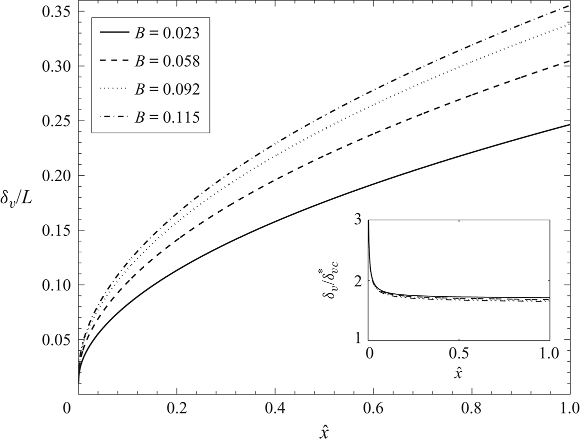
It is clear from figure 3 that blowing increases the velocity boundary layer thickness at a given  $\hat {x}$ since the height of the velocity profiles increase with increase in blowing strength. The corresponding spatial development of the velocity boundary layer for different
 $B$ is shown in figure 4. The fluid in the species boundary layer whose velocity is increased owing to blowing, as we saw above, drags more fluid from above it thereby resulting in an increased
 $\delta _v$ with
 $B$ at any
 $\hat {x}$. At any given
 $B$, the reason for the increased
 $\delta _v$ with
 $\hat {x}$ is also similar since
 $u$ increases with
 $x$. The inset of figure 4 shows the variation of
 $\delta _v/\delta _{vc}^*$ with
 $\hat {x}$ for different values of
 $B$, where
 \begin{equation} \delta_{vc}^*=Sc^{1/5}\left(\frac{\nu V_i x^{2}}{g\beta{\rm \Delta} C}\right)^{1/4}, \end{equation}
obtained by replacing  $L$ in (B 7) with
 $x$. All the profiles of
 $\delta _v/\delta _{vc}^*$ collapse to a single value of 1.75 implying similarity. Such a similarity implies that
 \begin{equation} \frac{\delta_{v}}{x} \simeq 1.75Sc^{1/5}\left(\frac{\nu V_i}{g\beta {\rm \Delta} Cx^2}\right)^{1/4} = 1.75Sc^{1/5} \frac{B^{5/4}}{Re_L}\sqrt{\frac{L}{x}}. \end{equation}
Hence,  $\delta _{vc}$ is the appropriate characteristic scale for the velocity boundary layer thickness.
Variation of the dimensionless velocity boundary layer thickness ( $\delta _{v}/L$) with the dimensionless horizontal coordinate
 $\hat {x}$ for various blowing parameter values. The inset shows that
 $\delta _v/\delta _{vc}^*$, where
 $\delta _{vc}^*$ is given by (3.8), is a constant equal to 1.75.

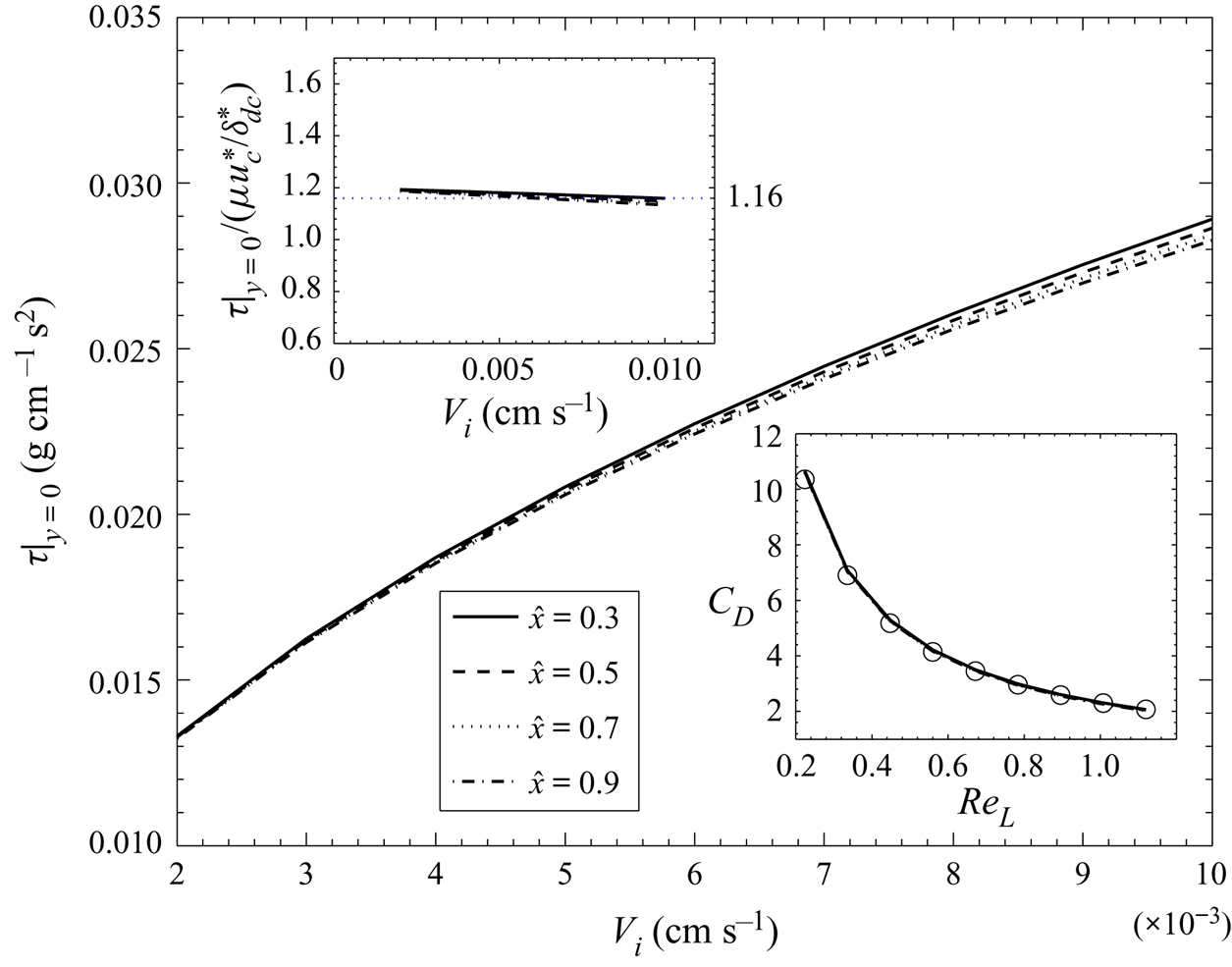
Figure 5 shows the variation of the wall shear stress with  $V_i$ at various
 $\hat {x}$, where the wall shear stress is defined as
 \begin{equation} \tau_{|y=0} = \mu \left. \frac{\partial u}{\partial y}\right |_{y = 0} \sim \rho\frac{\nu^2}{L^2}Sc^{-1/5}\frac{(Gr_LRe_L)^{1/2}}{\hat{\delta}_v} \left. \frac{\partial \hat{u}}{\partial \eta}\right |_{\eta = 0}, \end{equation}
and evaluated using the computed values of  $\hat {\delta }_d$ and
 $\hat {\delta }_v$. The wall shear stress increases with increase in
 $V_i$ at all
 $\hat {x}$; the dependence of
 $\tau |_{y=0}$ on
 $\hat {x}$ at any
 $V_i$ is quite weak. Note that the increase in wall shear stress at any
 $\hat {x}$, observed in figure 5, can also be observed in figure 3 as an increase in the vertical gradient of the velocity profile at the wall with increase in
 $B$. Weak blowing of lighter fluid increases the wall shear stress in NBL unlike in the case of weak blowing into shear boundary layers. In shear boundary layers the external forcing from the free stream flow creates the boundary layer, while it is the internal motion pressure gradient, due to the lighter fluid in the boundary layer, that drives the NBL. With an increase in the blowing velocity, within the weak blowing regime considered here, the dominant effect appears to be an increase in motion pressure gradient resulting in larger velocity gradients at the wall. The vertical momentum of blowing seems to be insufficient to reduce the velocity gradients at the wall at the low blowing velocities encountered in the present study.
Effect of blowing on the wall shear stress ( $\tau _{|y=0}$) at different dimensionless horizontal positions. The bottom, right inset shows the variation of the coefficient of drag
 $C_D$ with
 $Re_L$ at the different
 $\hat {x}$ with
 $\circ$ showing (3.13). The top, left inset shows the variation of
 $\tau _{|y=0}/(\mu \,u_c^*/\delta _{dc}^*)$ with
 $V_i$ at different
 $\hat {x}$ as in the main figure.

The top, left inset in figure 5 shows that the dimensionless wall shear stress,
 \begin{equation} \frac{\tau_{|y=0}}{(\mu u_c^*/\delta_{dc}^*)} \simeq 1.16, \end{equation}
is independent of  $V_i$ and
 $\hat {x}$, where
 $\tau _{|y=0}$ is calculated from (3.10), with
 $\delta _{dc}^*$ and
 $u_c^*$ given by (3.1) and (3.5), respectively. Using the expression for
 $\tau _{|y=0}$ from (3.11) in the expression for the coefficient of drag,
 \begin{equation} C_D = \frac{\tau_{|y=0}}{\rho u_c^2/2} \end{equation}
and simplifying using (B 6), (3.1) and (3.5), we obtain
 \begin{equation} C_D\simeq \frac{2.32}{Re_L}, \end{equation}
independent of  $\hat {x}$. As shown in the bottom, right inset of figure 5,
 $C_D$ calculated using (3.12), with
 $\tau _{|y=0}$ estimated by (3.10) using the computed velocity profiles, shows a good match with (3.13) for all
 $\hat {x}$. Hence, in laminar natural convection boundary layers with blowing, for
 $Re_{\delta _v}< 1$ and
 $0.012<B<0.12$, the coefficient of drag varies as
 $Re_L^{-1}$ unlike in laminar shear boundary layers, where the average coefficient of drag varies as
 $Re_L^{-1/2}$ (Schlichting & Gersten Reference Schlichting and Gersten2017). The relation (3.13) also implies that the drag coefficient based on
 $u_\nu$,
 \begin{equation} C_{D_{\nu}}= \frac{\tau{|_{y=0}}}{\rho u_\nu^2/2} = 2.32\sqrt{Gr_x Re_x}, \end{equation}
which clearly shows that both blowing and natural convection effects increase the drag.
3.4. Theoretical mean concentration profile
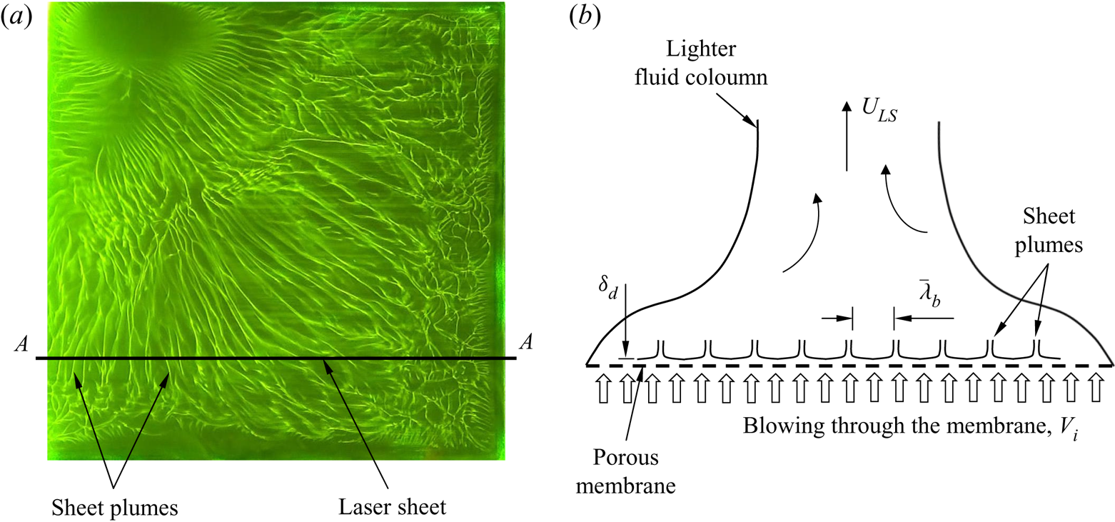
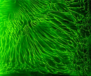
Experimental verification of the expressions (3.2), (3.7), (3.9) and (3.13) pose considerable difficulties, since, in addition to being thin ( ${\sim }0.3$ mm), these boundary layers are also unstable beyond a certain horizontal distance (PA08). As shown in figure 1(b), plumes arise from the instability of these boundary layers. Figure 6(a) shows the instantaneous top view of the region close to a horizontal membrane in an experiment where lighter water is forced from below the membrane at a velocity of
 $V_i=0.002$ cm s
 $^{-1}$, into a layer of heavier brine above the membrane. The light green lines in the image are the line plumes created by the instability of the natural convection boundary layers in between these plumes, which are subjected to a transpiration through the membrane. In addition to the fact that the boundary layer lengths are spatially random, the flow induced by these plumes causes these plumes to keep merging (Gunasegarane & Puthenveettil Reference Gunasegarane and Puthenveettil2014) so that the random pattern in figure 6(a) keeps evolving spatially and temporally with time. These boundary layers then form and are destroyed by the plume motion at various random locations and at various temporal instants above a horizontal porous surface. Due to this reason, identifying an individual boundary layer and measuring its profile is difficult in the parameter regime at which these boundary layers exist.
(a) Top view of the near-membrane sheet plumes observed in a forcing experiment with  $V_i = 0.002$ cm s
 $^{-1}$ and
 $Ra=8.1\times 10^{11}$. The spatial and temporal evolution of these sheet plumes is shown in supplementary movie 1, available at https://doi.org/10.1017/jfm.2020.603. (b) Schematic of the idealised distribution of the sheet plumes in the laser sheet plane
 $A$–
 $A$ in (a) when viewed from the front. Figure 8 shows the front view images of the actual sheet plume distribution obtained in such laser sheet planes in experiments with different blowing velocities.

In spite of this difficulty, indirect experimental verification of the expression for the species boundary layer thickness (3.2) could be obtained as follows. For steady convection, at any instant, the distances over which these boundary layers exist on the surface are distributed lognormally (PA08, Ramareddy & Puthenveettil Reference Ramareddy and Puthenveettil2011). However, there exist a mean spacing between the plumes,
 \begin{equation} \bar{\lambda}_b = 2K^{2/3}Sc^{1/6}\sqrt{Z_wZ_{V_i}}, \end{equation}
where  $K = 0.325$, equal to twice the mean distance over which the boundary layer forms on the surface (PA08, Ramareddy & Puthenveettil Reference Ramareddy and Puthenveettil2011). (Note that we define
 $\bar {\lambda }_b$ as the edge to edge distance between the adjacent plumes, unlike in the case of PA08 where
 $\bar {\lambda }_b$ is defined as the centre to centre distance of plumes. The present definition is more appropriate since (3.15) is obtained from relations that are valid only for boundary layers and not for regions within plumes.) For a given
 $B$, the actual spatial distribution of boundary layers over the surface in steady state could then be represented by an idealised distribution of pairs of boundary layers each of length equal to
 $\bar {\lambda }_b/2$ and facing each other (see figure 6b). The spatial average profiles in such an idealised representation should be the same as that in the actual case, which gives us an easy way to verify the theoretical profiles by comparing the spatial mean profile from such an idealised distribution with the spatial mean from the experiments. With such an aim to compare with experiments, we now derive the theoretical spatial mean concentration profile using the expression for the species boundary layer thickness (3.2) when the boundary layers become unstable at a constant horizontal distance
 $\bar {\lambda }_b/2$, given by (3.15). Interestingly, we find that the theoretical mean concentration profile becomes independent of the blowing velocity in the specific regime of convection that we discuss here.
Assuming that the boundary layer of length  $\bar {\lambda }_{b}/2$ repeats itself spatially, the horizontally averaged, steady state, concentration at any
 $y$ between the surface and the maximum species boundary layer thickness could be calculated as
 \begin{equation} \langle C(y)\rangle =\frac{1}{\bar{\lambda}_{b}/2} \int_{0}^{\bar{\lambda}_{b}/2}C(y)\,\mathrm{d}x, \end{equation}
by averaging the local concentration  $C(y)$ over a horizontal distance of
 $\bar {\lambda _b}/2$, along the horizontal line at a height of
 $y$, as depicted in figure 1(a). Let
 $x_d(y)$ be the horizontal distance at any
 $y$ at which the concentration changes from
 $C_{T}$ to
 $C_{B}$ (see figure 1a). Then, at any fixed
 $y$, splitting the integral over
 $\bar {\lambda }_b/2$ in (3.16) into integral from 0 to
 $x_d(y)$ over which the concentration is
 $C_{T}$ (white region in figure 1a), and from
 $x_d(y)$ to
 $\bar {\lambda _b}/2$ over which the concentration is
 $C_{B}$ (yellow region in figure 1a),
 \begin{equation} \langle C(y)\rangle = \frac{1}{\bar{\lambda}_{b}/2}\left(\int_{0}^{x_{d}(y)} C_{T}\,\mathrm{d}x + \int_{x_{d}(y)}^{\bar{\lambda}_{b}/2} C_{B}\,\mathrm{d}x\right). \end{equation}
Equation (3.17) simplifies to
 \begin{equation} \langle C(y)\rangle=C_{B}+\frac{2x_d}{\bar{\lambda}_b}{\rm \Delta} C. \end{equation}
The dimensionless, horizontally averaged, steady state, theoretical concentration at a height  $y$ can now be written from (3.18) as
 \begin{equation} \langle C^{*}(y)\rangle = \frac{\langle C(y)\rangle - C_{B}}{{\rm \Delta} C}= \frac{2x_d}{\bar{\lambda}_b}. \end{equation}
Since the height  $y$ at a horizontal distance of
 $x_d$ at which
 $C_{T}$ changes to
 $C_{B}$ is the same as
 $\delta _d(x_d)$, substituting
 $\delta _d=y$ and
 $x=x_d$ in (3.2), we obtain
 \begin{equation} x_{d} = \left(\frac{y}{1.6}\right)^{2} \sqrt{\frac{g\beta {\rm \Delta} C}{\nu V_i}}. \end{equation}
Using (3.20) and the expression for  $\bar {\lambda _b}$ given by (3.15) in (3.19), we obtain
 \begin{equation} \langle C^*(y)\rangle =\frac{0.39}{K^{2/3}Sc^{2/3}}\left(\frac{y}{Z_w}\right)^2= \frac{0.39}{K^{2/3}} Gr_y^{2/3}, \end{equation}
where  $Z_w$ is given by (3.4a) and
 $Gr_y=g\beta {\rm \Delta} C y^3/\nu ^2$ is the Grashof number based on
 $y$. Surprisingly, (3.21) implies that the dimensionless, horizontally averaged, steady state concentration profile within the boundary layer is independent of the strength of blowing. The profile is also independent of the species diffusion within the boundary layer, a consequence of blowing which creates a uniform concentration profile within the boundary layer. The boundary layer thicknesses and the velocity profile at any spatial location are functions of the blowing velocity (see (3.2) and (3.7)), but the horizontal average of the concentration profile becomes independent of
 $V_i$. This surprising independence of the horizontally averaged concentration profile on the strength of blowing is a consequence of the similar
 $1/\sqrt {V_i}$ dependence of
 $x_d$ and
 $\bar {\lambda }_b$, as shown by (3.20) and (3.15). We now see whether this predicted theoretical mean concentration profile can be obtained in experiments, if so, thereby indirectly verifying the relation (3.2).
4. Experiments
For verifying the theoretical expression of the mean concentration profile (3.21), two types of experimental set-ups that provide density difference across a horizontal membrane were used. While in the first set-up a gravitational head drives the flow through the membrane, it is the unstable density difference across the membrane that drives the flow in the second set-up. In both the experiments the PLIF technique was employed to extract the mean concentration distribution in a vertical plane near the membrane so that the experiments could be compared with the theory.
4.1. Set-up
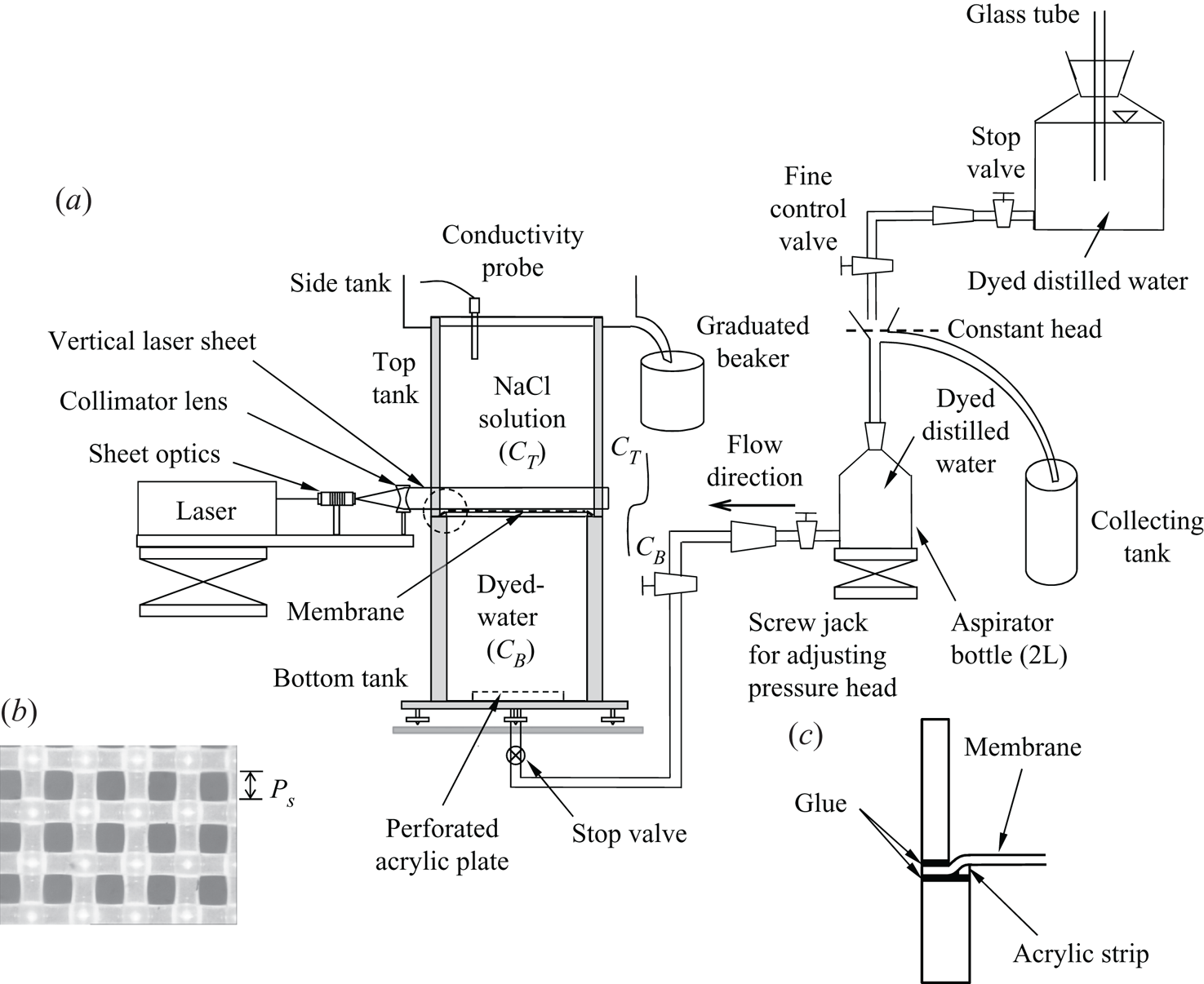
In both set-ups the arrangement consisted of a heavier layer of brine above a horizontal porous membrane, with a lighter layer of water, that had 0.48 parts per million (or p.p.m.) of Rhodamine-6G dye in it, below the membrane. In the first set-up, whose schematic is shown in figure 7(a), the bottom fluid was forced upwards through the membrane by the constant gravitational head arrangement shown in the figure. The porous membrane with a pore size  $P_s=45.6\ \mathrm {\mu }$m and an open area factor
 $\varGamma =0.31$ (figure 7b) was fixed as shown in figure 7(c). Such a fixture prevented the shadow cast by the glue from falling on the membrane surface when a vertical collimated laser sheet (Litron
 Nd:Yag laser, 532 nm, 100 mJ pulse
 $^{-1}$ and 50 Hz) was passed grazing the upper surface of the membrane. Due to this arrangement, the inner cross-section of the top tank was
 $15.6\ \mathrm {cm}\times 15.6\ \mathrm {cm}$ while that of the bottom tank was
 $15\ \mathrm {cm}\times 15\ \mathrm {cm}$; the heights of the fluid layers in the top and the bottom tanks were equal to
 $25.85\ \mathrm {cm}$ and
 $23.9\ \mathrm {cm}$, respectively. A CCD camera (ImagerProx4M, LaVision GmbH, not shown in figure 7) was mounted perpendicular to the vertical plane of the near-membrane region such that the image resolutions of the first and the second experimental configurations are 31 and 26 pixels mm
 $^{-1}$, respectively.
(a) Schematic of the experimental setup used in the present study; (b) magnified view of the porous membrane used in the experiments with pore size,  $P_s = 45.6\ \mathrm {\mu }$m and open area factor,
 $\varGamma = 0.31$, and (c) the magnified view of the arrangement used to prevent a shadow over the membrane in the region enclosed by the dashed circle in (a).

The bottom tank was filled with dyed water up to the membrane and the membrane was covered with a cling film before filling the top tank with brine. The experiment was initiated by removing the cling film which prevented mixing while the top tank was being filled. The bottom lighter fluid was then forced upwards through the membrane by the constant gravitational head arrangement shown in figure 7(a); we call these experiments the forcing experiments. The flow through the membrane was controlled by adjusting the gravitational head to conduct experiments with the desired uniform velocity  $V_i$ through the membrane which was maintained constant with respect to time
 $t$; the range of
 $V_i$ was chosen to be within the range of
 $V_i$ given in table 1. The volume of brine that leaves the top tank was measured for a specific time to calculate the uniform velocity of water flow through the membrane pores. The experiments were unsteady since the concentration of salt in the top tank decreased continuously with time, while the bottom tank had a constant, zero, salt concentration. However, quasi-steady approximation could be used to estimate the horizontally averaged concentration near the membrane, as shown in appendix E. In the present study, experiments were conducted with the concentration of NaCl in the top tank before the start of the experiment
 $(C^0) \simeq 11$ gl
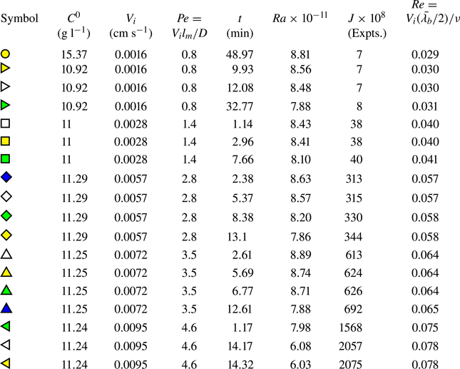
 $^{-1}$ for five velocities as shown in table 3.
List of parameters corresponding to the experiments conducted in the present study. Yellow circle, no-forcing experiment; all other symbols show forcing experiments.

The second experimental set-up was the same as the first one except that it did not have the arrangement beyond the stop valve at the inlet to the bottom tank shown in figure 7(a). The heights of the fluid layers in both the tanks were equal to  $23.9\ \mathrm {cm}$. These experiments were conducted with the stop-valve closed after the bottom tank was filled, and, hence, we call these experiments the no-forcing experiments. In these experiments, the concentration of NaCl in the top tank decreases with time from its initial value at the start of the experiment of
 $C^0\simeq 15$ gl
 $^{-1}$, while that in the bottom tank increases with time till eventual density equalisation occurs after 2.5 days approximately. In these experiments
 $V_i$ decreases with time and occurs due to the impingement of the large-scale flow on the membrane. Quasi-steady approximation in calculating the mean concentration profile could also be used in these experiments, as shown in detail in Ramareddy & Puthenveettil (Reference Ramareddy and Puthenveettil2011). Detailed descriptions of the no-forcing experiments are given in Puthenveettil (Reference Puthenveettil2004); Puthenveettil & Arakeri (Reference Puthenveettil and Arakeri2005, Reference Puthenveettil and Arakeri2008); Ramareddy & Puthenveettil (Reference Ramareddy and Puthenveettil2011). The parameters corresponding to this experiment (yellow circle) are shown in table 3.
4.2. Diagnostics
The spatial concentration maps of NaCl  $(C_e(x,y))$ at any time instant near the top of the membrane, in both set-ups, were calculated from the images of the fluorescence of the dyed, lighter bottom fluid crossing the vertical laser sheet grazing the membrane, as discussed in appendix F. Hereinafter, the subscript
 $e$ denotes the experimental values obtained from PLIF. Since
 $({\rm \Delta} \rho /\rho )_{\mathrm {dye}} \ll ({\rm \Delta} \rho /\rho )_{\mathrm {salt}}$, and since
 $Sc_{\mathrm {dye}}\gg Sc_{\mathrm {salt}}$ (
 $2000\gg 600$), the dye behaves as a passive scalar; the concentration of the dye will be equal to the concentration of the lighter fluid carrying the dye in the present mixing experiments. A four pole conductivity probe (Radiometer Analytical, SAS), immersed at around 30 mm below the brine level in the top tank, was used to measure the electrical conductivity of the top tank solution with time. The bulk concentration in the top tank was calculated from these conductivity measurements using standard relations (Lide Reference Lide2003); the Rayleigh number (
 $Ra = g\beta {\rm \Delta} C_eH^3/\nu D$) could then be calculated once
 ${\rm \Delta} C_e$ is obtained, as discussed in appendix G. The CCD camera and the conductivity meter were synchronised so that the Rayleigh number corresponding to the PLIF images would be known. The effect of Rhodamine-6G on the measured conductivity of the salt solution is negligible due to the low concentration of the dye used (Ramareddy Reference Ramareddy2009). Both experiments were started by removing the cling film. Initial mixing caused the concentration of NaCl in the top tank measured by the conductivity probe to fall from
 $C^0$ to values
 $C_p(t_s)$, slightly lesser than
 $C^0$, within a time
 $t_s$ of a few seconds, after which
 $C_p(t)$ starts to decrease monotonically. Hereinafter, the subscript
 $p$ denotes the experimental data obtained from the conductivity probe, different from that obtained from the PLIF data.
5. Comparison of the theoretical relations (3.2) and (3.21) with experiments
5.1. The dimensionless parameter in experiments
As seen in (2.19), the boundary layer thicknesses and the velocity profile, for a given fluid, depends only on  $B$. The analysis in § 3 was for a length
 $L$ of a steady boundary layer satisfying
 $0.012\leq B\leq 0.12$ at large
 $Sc$. However, in reality, these boundary layers become plumes after a mean distance of
 $L = \bar {\lambda }_b/2$, where
 $\bar {\lambda }_b$ is given by (3.15), beyond which the analysis of § 3 is not valid. Replacing
 $L$ in (2.21) with
 $\bar {\lambda }_b/2$ from (3.15), we obtain the blowing parameter in experiments
 $(B_e)$, based on
 $\bar {\lambda }_b$, the actual length over which the boundary layer exists as
 \begin{equation} B_e = \left(KJ\right)^{4/15}, \end{equation}
where
 \begin{equation} J = \frac{B^5}{Re_L^2} = \frac{Vi^3}{g\beta {\rm \Delta} C\nu} = \frac{Re_L^3}{Gr_L} \end{equation}
is an equivalent, length independent, dimensionless blowing parameter which decides the nature of these boundary layers. Here  $J$ is a dimensionless number showing the relative importance of blowing, buoyancy and viscous effects in the boundary layer, devoid of any length scale. The range of
 $J$ (
 $2\times 10^{-8} \leq J \leq 1.62\times 10^{-5}$) corresponding to the range of
 $B$ is shown in table 1. Expressions for the species boundary layer thickness (3.2), the horizontal velocity profile (3.7) and the drag coefficient (3.13) can now be rewritten in terms of
 $J$ by using (5.1) to obtain
 \begin{gather} \frac{\delta_d}{x} = \frac{1.6}{\sqrt{2}}\left(\frac{\sqrt{J}}{Re_x}\right)^{1/2}, \end{gather}
 \begin{gather}\frac{u}{V_i} = \sqrt{2}f(\eta)\frac{1}{\left(Re_x\sqrt{J}\right)^{1/2}},\quad \mathrm{and} \end{gather}
 \begin{gather}\frac{\tau_{|y=0}}{\rho V_i^2/2}=\frac{2.32}{\sqrt{J}}. \end{gather}
Hence, unlike in (3.2), (3.9) and (3.7) where  $\delta _d$,
 $\delta _v$ and
 $u$ are functions of
 $L$, due to the instability constraint (3.15), these variables are in actuality only functions of
 $J$ and
 $Re_x$. Hence, the range of
 $J$ in experiments and in theory have to be the same to ensure that the uniform concentration approximation is valid in both cases. Tables 1 and 3 show that the range of
 $J$ is the same in theory and experiments. Furthermore, as we saw in § 3.4, the horizontal averaging of the concentration profile over their instability distance (3.15) makes the theoretical mean profile (3.21) independent of
 $V_i$ also. A comparison of the theoretical species boundary layer thickness (3.2) and the theoretical mean concentration profile
 $\langle C(y)\rangle$ with the corresponding experimental values,
 $\delta _{de}$ and
 $\langle C_e(y)\rangle$, respectively, at an instant needs to be then done by matching only the driving concentration difference
 $({\rm \Delta} C_e(t))$ and the fluid properties; we achieve this as we describe below.
5.2. Spatial concentration maps
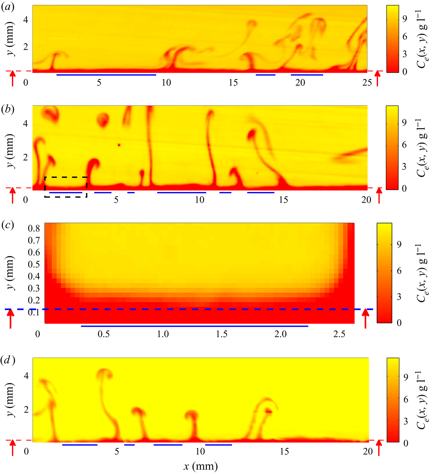
Figure 8 shows the spatial maps of concentration of NaCl ( $C_e(x,y)$) in the near-membrane region for
 $J =7\times 10^{-8}, 3.8\times 10^{-7}$ and
 $6.24\times 10^{-6}$ at various specific instants of time. The parameters corresponding to these concentration maps (yellow right-pointing triangle, square and upward-pointing triangle, respectively) are given in table 3. The horizontal red color regions, approximately 0.3 mm thick, near the bottom of each image are the boundary layers on the membrane. The location of the membrane in the PLIF images (
 $y=0$ in the images in figure 8) were fixed by first imaging the region without the laser sheet. The near-vertical red streaks show the sheet plumes in the yellow background of the bulk fluid. The blue lines at the bottom indicate the horizontal distance between the adjacent plumes,
 $\lambda_e$.
The spatial concentration distribution of NaCl in the near-membrane region for some of the experiments shown in table 3: (a) yellow right-pointing triangle,  $J = 7\times 10^{-8}$ (time,
 $t = 9.93$ min); (b) yellow square,
 $J = 3.8\times 10^{-7}$ (
 $t = 2.96$ min); (c) magnified view of the region surrounded by the rectangle shown in (b); (d) yellow upward-pointing triangle,
 $J = 6.24\times 10^{-6}$ (
 $t = 5.69$ min), where
 $J$ is given by (5.2). The spatial and temporal evolution of the sheet plumes in (b) is shown in supplementary movie 2. The time
 $t$ shown corresponds to the time at which the image was recorded after the start of the experiment. The blue lines at the bottom show the distances used for averaging, and the red arrow points to the location of the first valid data point, whereas
 $y=0$ refers to the top surface of the membrane.

The zoomed view of the region above the first red line in figure 8(b), shown in figure 8(c), shows the increasing concentration of NaCl,  $C_{e}(x,y)$ at
 $t = 2.96$ min from a lower value near the membrane to a higher value in the bulk. The experimental spatial mean concentration values of NaCl,
 $\langle C_{e}(y)\rangle$ at the instant of these images, is obtained by averaging from such regions between the plumes in each image. However, in spite of the laser sheet being collimated and carefully aligned parallel to the membrane, due to the reflection of laser light from the membrane, our mean concentration measurements are not reliable within a distance of approximately
 $h_l=0.12$ mm from the membrane surface. At distances less than
 $h_l$ from the membrane, the mean profiles deviated from the expected decreasing trend towards the membrane; we exclude these anomalous data in our mean concentration curves; the red dashed lines with vertical arrows on both sides of the images in figure 8 point to the location of the first valid data point.
5.3. Matching of  ${\rm \Delta} C$ in theory and experiments

Since the estimation of concentration very close to the membrane region in experiments is erroneous, the value of concentration at the bottom of the boundary layer  $C_{Be}(t)$ calculated from PLIF and, hence, the estimated driving concentration difference from PLIF would be erroneous;
 $C_{Be}(t)$ cannot also be taken to be zero due to the initial mixing. Hence, the values of
 $C_{Be}(t)$ for both the experiments are estimated using the concentrations calculated from the conductivity probe measurements as follows. For the no-forcing experiments,
 $C_{Be}(t)$ is calculated using both the conductivity probe measurements and the PLIF images as explained in appendix G.1. This
 $C_{Be}(t)$ is used as the bottom concentration in both the theoretical and experimental profiles. For the forcing experiments, as explained in appendix G.2, we calculate
 $C_{Be}(t)$ using (G 6) obtained from the mass balance in the bottom tank, and use these as the bottom concentration in the theoretical and experimental concentration profiles.
The horizontally averaged concentration at an instant,  $\langle C_e(y)\rangle$, above a height of 0.8 mm from the membrane surface, calculated from the PLIF images was found to be spatially constant; we hence choose this uniform concentration as the concentration above the boundary layer for both the forcing and the no-forcing experiments in theoretical and experimental profiles. Therefore, for each experimental set-up, the theoretical and experimental mean concentration profiles are compared by using the corresponding driving concentration difference
 ${\rm \Delta} C_e(t) = \langle C_{e}(y = 0.8\ \mathrm {mm})\rangle - C_{Be}(t)$, with
 $C_{Be}(t)$ estimated from conductivity measurements at the same instant as the PLIF image, as described above.
5.4. Comparison of species boundary layer thicknesses
Using the spatial concentration maps similar to those shown in figure 8, we measure the local, instantaneous, experimental species boundary layer thicknesses  $\delta _{de}$ as follows. As could be seen from figure 6(a), the boundary layers are all not perpendicular to the laser sheet. Furthermore, as seen from figure 8, their lengths of intersection with the laser sheet also vary, possibly due to the random nature of perturbations which affect their instability. In addition, some of the boundary layers appear spatially perturbed, possibly due to the accumulation of fluid due to the lateral motion of plumes. To avoid these complications affecting the measurements, from each image at each
 $V_i$, we judiciously choose pairs of adjacent plumes that are approximately separated by 1 cm and bounding boundary layer regions that are free of waviness. Since we expect the boundary layer pair between the plumes to grow equally in the opposite horizontal directions from the centre of the region between the plumes, we choose the leading edge of each boundary layer to be at the mid point of the distance between the plume pair. Since species boundary layer in the present experiments is approximately 0.3 mm thick (see figures 8c and 10), we horizontally average the concentration between each plume pair at
 $y\sim 0.3$ mm and assign the result as
 $C_{Te}$ for finding the edge of the species boundary layer. At each
 $x$ location within the length of the boundary layer, the maximum height of the pixels whose concentration is less than
 $C_{Te}$ is then taken to be
 $\delta _{de}(x)$.
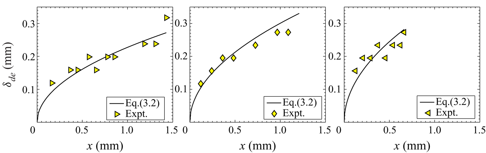
Figure 9 shows the variation of  $\delta _{de}$ at three different values of
 $J$ in experiments. As expected from the theory, larger blowing velocities result in larger
 $\delta _{de}$ and its longitudinal gradient at any
 $x$. The figure also shows the variation of the theoretical species boundary layer
 $\delta _d$, (3.2), calculated using the local
 ${\rm \Delta} C_e = C_{Te} - C_{Be}$, with
 $C_{Be}$ estimated using (G 6). As we can see, the measurements match fairly well with (3.2) at all the three
 $J$ considered; similar match of
 $\delta _{de}$ and
 $\delta _d$ were obtained at the
 $J$ listed in table 3. Considering the non-idealities mentioned above in these measurements, it is remarkable that a good match between
 $\delta _{de}$ and
 $\delta _d$ (3.2) is obtained. This match of
 $\delta _{de}$ and
 $\delta _d$ (3.2) validates the scaling theory presented in § 3.
Measured species boundary layer thicknesses in the experiments ( $\delta _{de}$) as a function of the streamwise distance (
 $x$). Yellow right-pointing triangle,
 $J = 13\times 10^{-8}$ (
 $V_i = 0.0016\ \mathrm {cm\ s}^{-1}$); yellow diamond,
 $J = 507\times 10^{-8}$ (
 $V_i = 0.0057\ \mathrm {cm\ s}^{-1}$); yellow left-pointing triangle,
 $J = 2577\times 10^{-8}$ (
 $V_i = 0.0095\ \mathrm {cm\ s}^{-1}$). The solid curves are the corresponding expressions (3.2), calculated using the local
 ${\rm \Delta} C_e$ of the boundary layer considered.

5.5. Comparison of mean concentration profiles
The experimental mean concentration profile was calculated by averaging the concentration in the boundary layer region over distances between the edges of the plumes, for similar values of  $J$ as in the theory, for the same values of
 ${\rm \Delta} C$. The averaging is done over several plume pairs in each image with the number of plume pairs ranging from three to nineteen for different
 $J$, based on the availability of clear boundary layer regions. As shown in § 3.4, the theoretical mean concentration profile (3.21) was obtained by assuming no concentration drop in the species boundary layer. Such a regime of convection has been studied earlier by PA08, which they termed as the advection regime, which occurs when the Peclet number
 $Pe=V_il_m/D\gtrsim 0.8$, where
 $l_m$ is the thickness of the membrane. As shown in table 3, comparisons of (3.21) with the experimental profiles are done only for experiments in which
 $Pe \ge 0.8$.
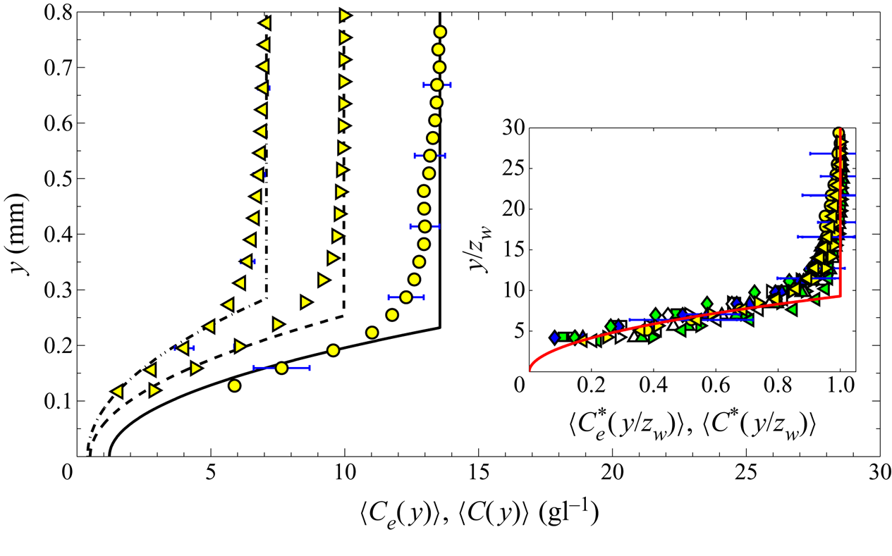
Figure 10 shows the mean experimental concentration profiles of NaCl,  $\langle C_e(y)\rangle$, obtained by horizontally averaging the spatial concentration distribution
 $C_e(x,y)$ in the concentration maps, similar to that shown in figure 8, for
 $J= 7\times 10^{-8}, 7\times 10^{-8}$ and
 $2.1\times 10^{-5}$ at the instant shown in table 3. The errors in
 $\langle C_e(y)\rangle$, estimated as the standard deviation normalised by the square root of the sample number, are shown as the error bars. The curves for the no-forcing (yellow circle) and the forcing (yellow right-pointing triangle) experiments show that at the same blowing velocity, if the concentration difference is larger, the larger is the
 $Ra$ and the lower is the height of the concentration profile. These two data are at the same
 $J$, but differ in
 $Ra$; the profiles being quite different shows the strong dependence on
 $Ra$, though
 $J$ is the same. By comparing the data in figure 10 at
 $J=7\times 10^{-8}$ (yellow right-pointing triangle) with the data at
 $J=2.1\times 10^{-5}$ (yellow left-pointing triangle), it would appear that an increase in blowing increases the boundary layer thickness. However, the data at
 $J=2.1\times 10^{-5}$ is also at a much lower
 $Ra$, which could be the predominant reason for the increase in the height of the profile, and not the increase in the blowing velocity.
Mean concentration profile in experiments and theory for three of the experiments shown in table 3. No-forcing experiment: yellow circle,  $J = 7\times 10^{-8}$; forcing experiments: yellow right-pointing triangle,
 $J = 7\times 10^{-8}$; yellow left-pointing triangle,
 $2.1\times 10^{-5}$. Here –, – – and –
 $\cdot$ – represent the corresponding dimensional, theoretical concentration
 $\langle C(y)\rangle$ profiles obtained by using (3.21) in (3.19). The inset shows the dimensionless mean concentration data obtained from the experiments (symbols) for all the values of
 $J$ listed in table 3. The red curve is the dimensionless, theoretical mean concentration profile obtained using (3.21).

These trends become clearer by comparing these mean experimental profiles with the mean theoretical concentration profiles  $\langle C(y)\rangle$ calculated from (3.21), shown as lines in figure 10. The theoretical profiles are linear away from the membrane showing increasing importance of diffusion away from the membrane, while nonlinearity near the membrane shows the predominance of advection over diffusion; the height of the vertically varying part of the mean concentration profile indicates the mean species boundary layer thickness. A good match between the theoretical and experimental mean concentration profiles is seen in figure 10, except near the edge of the mean species boundary layer; a similar match was obtained for all the values of
 $J$ shown in table 3. The deviation of the upper part of
 $\langle C_e(y)\rangle$ from
 $\langle C(y)\rangle$ is expected to be due to the bulk concentration in experiments just above the boundary layers being slightly less than
 $C_{Te}$, contrary to the assumption in obtaining the theoretical profile, due to the local mixing from the rising and dispersing plumes near the boundary layers. It is also possible that the variation of boundary layer thickness with
 $x$ varies from that described by (3.2) close to the formation of plumes due to the boundary layers becoming unstable. The match of the experimental concentration profiles with the concentration profile obtained from (3.21) implies that since (3.21) is independent of the blowing velocities
 $V_i$, the mean experimental profiles must also be so.
This independence of the mean concentration profile on  $V_i$ and
 $D$ could be clearly seen in the inset of figure 10, where the mean experimental concentration profiles are plotted for all the values of
 $J$ (shown in table 3) in their dimensionless form
 $\langle C_{e}^*\rangle =(\langle C_{e}\rangle - C_{Be})/{\rm \Delta} C_e$ against the dimensionless vertical coordinate
 $y/Z_w$. The error bars show the estimated errors in
 $\langle C_{e}^*\rangle$, which are obtained by using the error in
 $\langle C_{e}\rangle$ and that in the conductivity measurements (2 % of the reading). All the dimensionless mean concentration profiles at
 $0.0016$ cm s
 $^{-1}\leq V_i\leq 0.0095$ cm s
 $^{-1}$ collapse on to the theoretical curve (3.21), which is independent of
 $V_i$ and
 $D$. This remarkable collapse of the concentration profiles at various blowing strengths is also an indirect verification of (3.2), given that (3.15) has been shown to match with experimental measurements by PA08.
6. Discussion and conclusions
The primary contributions of the present work include the relations for high Schmidt number ( $Sc$) natural convection boundary layers on horizontal surfaces subjected to a spatially constant weak blowing, which typically occur in concentration-driven convection in liquids bounded by porous surfaces. New relations were obtained for the boundary layer thicknesses (3.2), (3.9), the horizontal velocity profile (3.7) and the drag coefficient (3.13), which along with the stability length of such boundary layers, surprisingly imply that the mean concentration profile (3.21) becomes independent of the blowing. These scalings were obtained from the analysis of the solutions of the integral natural convection boundary layer equations with a constant blowing velocity as one of its boundary conditions for the case of high Schmidt numbers
 $Sc$, where, due to the very thin species boundary layers, a weak blowing creates a uniform concentration, the same as the concentration of the fluid blown into the boundary layers.
The species boundary layer thickness  $\delta _d\sim x(Re_x/Gr_x)^{1/4}$ (3.2), implying a dependence of the boundary layer thickness on buoyancy, viscous and the blowing forces, in contrast to the case of natural convection boundary layers with no blowing where
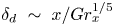 $\delta _d~\sim ~x/Gr_x^{1/5}$ (Pera & Gebhart Reference Pera and Gebhart1973). With stronger blowing, represented by a larger local blowing Reynolds number
 $Re_x$ based on the blowing velocity
 $V_i$ and the longitudinal distance
 $x$,
 $\delta _d$ was larger at any
 $x$. The scaling also implies that increasing the natural convection effects by increasing the local Grashof number
 $Gr_x$ based on
 $x$ would reduce
 $\delta _d$ at any
 $x$. If a local Blowing parameter is defined as
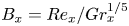 $B_x=Re_x/Gr_x^{1/5}$, which shows the relative local strength of blowing over natural convection and viscous effects, the above scaling (3.2) implies that
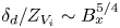 $\delta _d/Z_{V_i}\sim B_x^{5/4}$, where
 $Z_{V_i}=\nu /V_i$ is the viscous-advective length scale (Puthenveettil & Arakeri Reference Puthenveettil and Arakeri2008). In terms of the length scales near the membrane, the above scaling means that
 $\delta _d\sim (x^2Z_w^3Sc/Z_{Vi})^{1/4}$, while in the case of pure natural convection over a horizontal surface
 $\delta _d\sim (x^2Z_w^3Sc)^{1/5}$, where
 $Z_w$ is the near-wall length scale in turbulent convection (Puthenveettil et al. Reference Puthenveettil, Gunasegarane, Agrawal, Schmeling, Bosbach and Arakeri2011).
In reality, such boundary layers are unstable and would turn upwards to form plumes at a mean distance of  $\bar {\lambda }_b$ (Puthenveettil & Arakeri Reference Puthenveettil and Arakeri2008). We find that this instability condition, along with the presence of an approximately uniform concentration region of thickness
 $\delta _d$ on the porous surface implies that the horizontally averaged concentration profile, normalised by the driving concentration difference
 ${\rm \Delta} C$, should scale as
 $(y/Z_w)^2$ (3.21) with
 $y$ being the vertical coordinate. This scaling implies that the mean concentration profile across such boundary layers should become quadratic in
 $y$, independent of the strength of blowing, and be a function of only the driving concentration difference for a range of weak blowing velocities so that the blowing parameter
 $0.012<B=Re_L/Gr_L^{1/5}<0.12$. Such an inference is then verified experimentally by measurements of the spatial mean concentration profile on top of a horizontal membrane that separates brine above it from pure water below it, while a weak flow is forced through the membrane by gravity. The matching of the dimensionless mean concentration profile in experiments at different
 ${\rm \Delta} C$ and
 $V_i$ with (3.21), in addition to proving such a unique concentration profile, also indirectly verifies the proposed boundary layer scalings.
The velocity boundary layer thickness  $\delta _v\sim \delta _d Sc^{1/5}$ (3.9), proportional to
 $\delta _d$, while the horizontal velocity profile
 $u\sim V_i\, f(\eta ) (Gr_x/Re_x)^{1/4}$ (3.7), where
 $\eta =y/\delta _v$. The scaling of the horizontal velocity implies that
 $u/u_\nu \sim (Gr_x Re_x^3)^{1/4}$, where
 $u_\nu =\nu /x$ is the viscous velocity scale, showing a stronger effect of blowing than natural convection in changing the horizontal velocities. In contrast, in the absence of blowing,
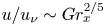 $u/u_\nu \sim Gr_x^{2/5}$ (Pera & Gebhart Reference Pera and Gebhart1973). With increase in blowing, since more lighter fluid accumulates close to the surface, thereby increasing the driving horizontal pressure gradient at the surface, the vertical gradient of the horizontal velocities at the surface increased with blowing. In consequence, the drag due to the boundary layer increased with stronger blowing, unlike that in the case of shear flows with transpiration. Such an increase of the drag with blowing was seen in the scaling of the drag coefficient based on
 $u_\nu$,
 $C_{D\nu }\sim \sqrt {Gr_xRe_x}$ (3.14); both natural convection and blowing has similar effects in increasing the drag of the boundary layers.
Even though the proposed new scalings for the boundary layer parameters for high  $Sc$ natural convection boundary layers on horizontal surfaces with a weak blowing are in general agreement with the solutions of integral equations and indirectly with the experiments, they also raise some interesting questions. Lack of similarity solutions for these boundary layer equations, except for a
 $x^{-2/5}$ variation of
 $V_i$ has been well known (Clarke & Riley Reference Clarke and Riley1975; Merkin Reference Merkin1975; Chen et al. Reference Chen, Buchanan and Armaly1993). The present study shows that similarity of the relevant boundary layer parameters might be possible for these boundary layers for a specific range of blowing velocities and concentration differences when
 $Sc$ becomes large, albeit with a different set of similarity variables and characteristic scales from those proposed by the earlier researchers. This aspect of the similar nature of these boundary layers needs to be further investigated. The present analysis is for boundary layers with a weak blowing so that inertial effects are negligible in the boundary layers, which is met by ensuring that the analysis is conducted only for the cases where Reynolds numbers based on
 $\delta _v$,
 $Re_{\delta _v}\ll 1$. Non-negligible inertial effects would imply that the characteristic scales (B 5) and (B 6) would no longer be valid; new scales will then have to be obtained and the subsequent analysis will have to be redone.
Acknowledgements
The authors gratefully acknowledge the financial support of DST, Government of India through their FIST grant SR/FST/ETII-017/2003 and their core research grant SR/S3/MERC/028/2009.
Declaration of interests
The authors report no conflict of interest.
Supplementary movies
Supplementary movies are available at https://doi.org/10.1017/jfm.2020.603.
Appendix A. Justification for the uniform concentration approximation
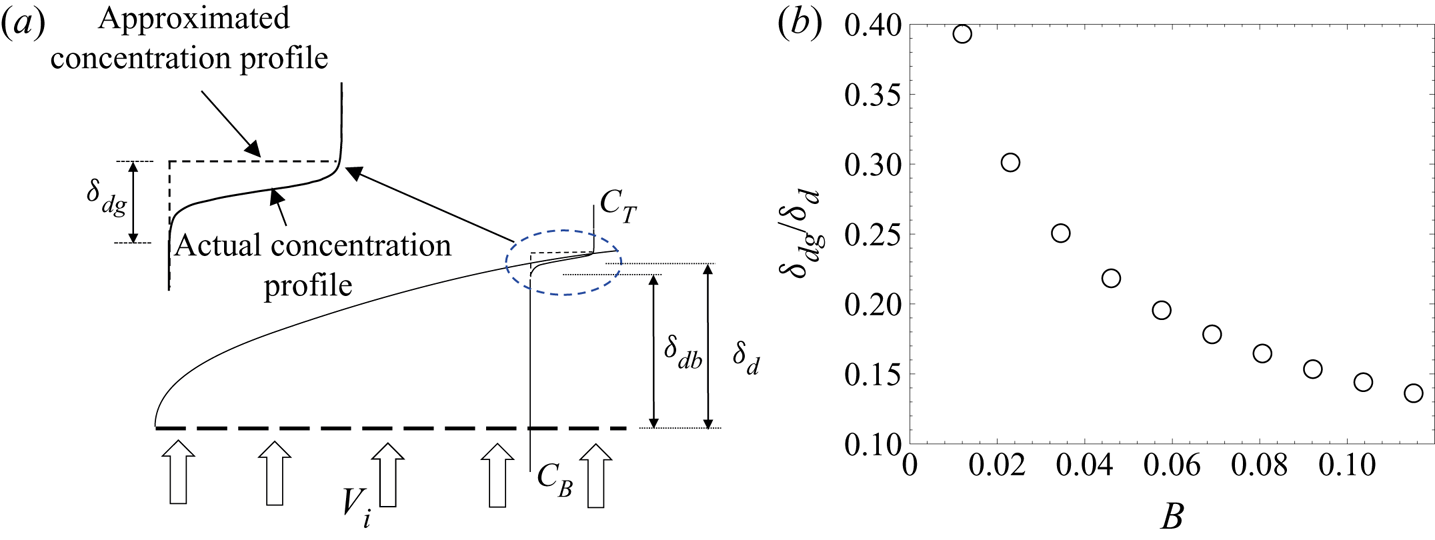
Figure 11(a) shows the concentration profile assumed in the integral analysis (dashed line) along with the expected actual concentration profile (solid line) in the species boundary layer. If  $\delta _{dg}$ and
 $\delta _{db}$ are the thicknesses of the regions within the species boundary layer that would, in reality, have a concentration gradient and a uniform concentration, respectively, then the uniform concentration approximation can be justified if
 $\delta _{dg}\ll \delta _{d}$. As we show below,
 $\delta _{dg} \ll \delta _{d}$ for the present range of study.
(a) The actual and approximated concentration profile in the species boundary layer. (b) Dependence of  $\delta _{dg}/\delta _{d}$ (A 5) on the blowing parameter.

From the steady mass balance in a control volume of height  $\delta _{db}$ and width
 $x$ in the uniform concentration region of the species boundary layer,
 \begin{equation} V_{i}x \sim \delta_{db}u_c, \end{equation}
where  $u_c$ is the horizontal characteristic velocity inside the control volume, defined later in (B 6). A balance of convection and diffusion in a control volume, of height
 $\delta _{dg}$ and width
 $x$, located in the gradient region of the species boundary layer implies that
 \begin{equation} D\frac{{\rm \Delta} C}{\delta_{dg}} x \sim u_c\delta_{dg} {\rm \Delta} C. \end{equation}
Rewriting  $\delta _{db}$ in (A 1) as
 $\delta _d - \delta _{dg}$, (A 1) becomes
 \begin{equation} \frac{\delta_{dg}}{\delta_{d}}\sim \frac{1}{\left(V_ix/u_c\delta_{dg}\right) + 1}. \end{equation}
Replacing  $\delta _{dg}$ on the right-hand side of (A 3) with
 $\sqrt {D\,x/u_c}$, obtained from (A 2), imply that at
 $x = L$,
 \begin{equation} \frac{\delta_{dg}}{\delta_{d}}\sim \frac{1}{1 + V_i\sqrt{L/u_cD}}. \end{equation}
Using the characteristic scales for horizontal velocity, (B 6), in (A 4) implies that
 \begin{equation} \frac{\delta_{dg}}{\delta_{d}} \sim \frac{1}{1 + \sqrt{B^{5/4}Sc}}, \end{equation}
where  $B$ is the dimensionless blowing parameter defined in (2.21). For
 $\delta _{dg}/\delta _{d}\ll 1$, (A 5) implies that
 $B^{5/4}Sc\gg 1$. Figure 11(b) shows the variation of
 $\delta _{dg}/\delta _{d}$ with
 $B$ as per (2.21) for the range of blowing velocity used in the present study, as listed in table 1. The ratio
 $\delta _{dg}/\delta _d\ll 1$ for
 $B\geq 0.012$, thereby validating the uniform concentration approximation. We hence restrict the lower limit of our analysis to
 $B=0.012$, the corresponding blowing velocity is
 $V_i\simeq 0.001\ \mathrm {cm\ s}^{-1}$.
Appendix B. Characteristic scales
The characteristic vertical velocity is  $V_i$, while the relevant characteristic horizontal length is
 $L$. An order of magnitude estimate of the integral momentum equation (2.17) gives
 \begin{equation} \frac{\delta_{vc}u_c^2}{L} - \frac{1}{2}g\beta{\rm \Delta} C\frac{\delta_{dc}^2}{L} + \nu \frac{u_c}{\delta_{dc}} \sim 0, \end{equation}
where and hereinafter the terms with subscript  $c$ indicate the characteristic scale of the corresponding quantity (Puthenveettil & Arakeri (Reference Puthenveettil and Arakeri2008), hereafter referred to as PA08). Similarly, the integral species equation (2.18) implies that
 \begin{equation} \frac{u_c\delta_{dc}}{L} \sim V_i. \end{equation}
Dividing (B 1) by its second term, and replacing  $u_c$ in the resulting equation with that from (B 2), we get
 \begin{equation} \frac{V_i^2L^2\delta_{vc}}{g\beta{\rm \Delta} C\delta_{dc}^4} + \frac{\nu V_iL^2}{g\beta{\rm \Delta} C\delta_{dc}^4} \sim 1. \end{equation}
In (B 3) the first term represents the ratio of the inertial forces to the motion pressure gradient, whereas the second term represents the ratio of the viscous forces to the motion pressure gradient. The ratio of the first and the second term in (B 3) is
 \begin{equation} Re_{\delta_v} = V_i\delta_{vc}/\nu. \end{equation}
When  $Re_{\delta _v} \ll 1$, which is the regime of the present study, the first term in (B 3) is negligible, implying that
 \begin{equation} \delta_{dc}\sim \left(\frac{\nu V_i L^2}{g\beta {\rm \Delta} C}\right)^{1/4} = L\left(\frac{Re_L}{Gr_L}\right)^{1/4}. \end{equation}
Substituting (B 5) in (B 2), the characteristic scale for the horizontal velocity becomes
 \begin{equation} u_c\sim \left(\frac{V_i^3L^2g\beta{\rm \Delta} C}{\nu}\right)^{1/4}= \frac{\nu}{L}\left(Gr_LRe_L^3\right)^{1/4}; \end{equation}
(B 5) and (B 6) were first obtained by PA08. Analysis of the numerical solution of the dimensionless integral equations by Ramareddy (Reference Ramareddy2009) revealed that the ratio  $\delta _d/\delta _v$ was approximately equal to
 $\simeq 0.27$ for the range of
 $V_i$ used in the present study. Since
 $Sc^{1/5}=0.27$ in the present study, based on our expectation that the velocity boundary layer thickness should scale similar to the species boundary layer thickness, we choose
 \begin{equation} \delta_{vc}\sim Sc^{1/5}\delta_{dc}; \end{equation}
a more rigorous order of magnitude analysis of (2.9) to (2.18) than done by Puthenveettil (Reference Puthenveettil2004) might give rise to this scaling.
Appendix C. Coefficients in (2.25), (2.28) and (2.29)
The values of  $K_{1}$,
 $K_{2}$,
 $K_{3}$ and
 $K_{4}$ in (2.25) are
 \begin{gather} K_{1} = 0, \end{gather}
 \begin{gather}K_{2} =\frac{Sc^{2/5}\hat{\delta}_{v}^2\hat{\delta}_{d}'} {4+B^{5/4}Sc^{1/5}\hat{\delta}_v}, \end{gather}
 \begin{gather}K_{3} = \frac{-2Sc^{2/5}\hat{\delta}_{v}^2\hat{\delta}_{d}'}{4+B^{5/4}Sc^{1/5} \hat{\delta}_v}, \end{gather}
 \begin{gather}K_{4} = \frac{Sc^{2/5}\hat{\delta}_{v}^2\hat{\delta}_{d}'} {4+B^{5/4}Sc^{1/5}\hat{\delta}_v}. \end{gather}
The coefficients in (2.28) and (2.29) are
 \begin{gather} E_{1} = \frac{B^{5/4}Sc^{6/5}\hat{\delta}_v^5(20+3B^{5/4}Sc^{1/5}\hat{\delta}_v)}{105(4+B^{5/4}Sc^{1/5}\hat{\delta}_v)^3}, \end{gather}
 \begin{gather}E_{2} = Sc^{1/5}\hat{\delta}_v\left(-\hat{\delta}_d+\frac{Sc^{1/5}\hat{\delta}_v}{4+B^{5/4}Sc^{1/5}\hat{\delta}_v}\right), \end{gather}
 \begin{gather}E_{3} = \frac{2B^{5/4}Sc^{6/5}\hat{\delta}_v^6}{105(4+B^{5/4}Sc^{1/5}\hat{\delta}_v)^2}, \end{gather}
 \begin{gather}E_{4} = \frac{\hat{\delta}_d(\hat{\delta}_d-Sc^{1/5}\hat{\delta}_v)^2}{Sc^{1/5}\hat{\delta}_v(4+B^{5/4}Sc^{1/5}\hat{\delta}_v)}, \end{gather}
 \begin{gather}E_{5} = \frac{\hat{\delta}_d^2(-6\hat{\delta}_d^2-3B^{5/4}Sc^{1/5}\hat{\delta}_d^2 \hat{\delta}_v+4Sc^{2/5}(3+B^{5/4}\hat{\delta}_d)\hat{\delta}_v^2)}{6Sc^{1/5} \hat{\delta}_v^2(4+B^{5/4}Sc^{1/5}\hat{\delta}_v)^2}, \end{gather}
 \begin{gather}E_{6} = \frac{3\hat{\delta}_d^4-8Sc^{1/5}\hat{\delta}_d^3\hat{\delta}_v+6Sc^{2/5} \hat{\delta}_d^2\hat{\delta}_v^2}{48Sc^{1/5}\hat{\delta}_v+12B^{5/4} Sc^{2/5}\hat{\delta}_v^2}. \end{gather}
Appendix D. Estimation of Prandtl–Blasius velocity profile
In the transpiration case, corresponding to  $B=0.12$, the Reynolds number based on the boundary layer length (
 $L=1$ cm) is
 $Re_L= 1.12$ (see table 2). Using (2.21) and since
 $Gr_L=Ra_LSc$, the Rayleigh number based on the boundary layer length in the transpiration case is
 \begin{equation} Ra_L=\left(\frac{Re_L}{B}\right)^5Sc =4.26\times 10^7. \end{equation}
The near-wall Rayleigh number based on the width of the fluid layer,  $W=15.6$ cm, is then
 \begin{equation} Ra_w=Ra_L\left(\frac{W}{L}\right)^3=1.61\times 10^{11}. \end{equation}
Here,  $W$ is chosen to be the width of the tank in the present experiments (see § 4.1). The large-scale flow Reynolds number corresponding to this
 $Ra_w$ is calculated using
 \begin{equation} Re_{LS}=0.55Ra_w^{4/9}Pr^{-2/3}\simeq 740, \end{equation}
given by Gunasegarane & Puthenveettil (Reference Gunasegarane and Puthenveettil2014). The corresponding large-scale flow velocity is  $U_{LS}=0.42\ \mathrm {cm\ s}^{-1}$. Using
 $U_{LS}$ as the free stream velocity of a steady, uniform flow over a horizontal plate, the Blasius profile is calculated by numerically solving the ordinary differential equation for the dimensionless streamfunction given by Schlichting & Gersten (Reference Schlichting and Gersten2017) as
 \begin{equation} f''' + ff'' = 0. \end{equation}
The boundary conditions used are
 \begin{gather} \eta_{B} = 0 : f = 0,\quad f' = 0, \end{gather}
 \begin{gather}\eta_{B} \rightarrow \infty : f' = 1. \end{gather}
Here,  $f(\eta _{_B}) = \psi /\sqrt {2\nu xU_{LS}}$,
 $\eta _{B}=y\sqrt {U_{LS}/(2\nu x)}$ is the similarity variable,
 $\psi$ is the dimensional streamfunction and
 $'$ denote differentiation with respect to
 $\eta _{B}$. The blue curve in figure 3 represents the dimensional Blasius profile,
 $u(x,y) = f'(\eta _{B})U_{LS}$, plotted against
 $y$ at a streamwise distance
 $x =W/2$ from the leading edge.
Appendix E. Quasi-steady approximation
The theoretical analyses in §§ 2 and 3 are conducted for a steady NBL with transpiration while in experiments the bulk concentration,  $C_{Te}$, keeps decreasing with time. However, the boundary layers in the experiments are quasi-steady since the boundary layers see an almost constant bulk concentration during their lifetime. This is so because the time scale of change of bulk concentration
 $t_c = C_T/(\mathrm {d}C_T/\mathrm {d}t)$ is much larger than the time scale of boundary layers
 $t_b = \delta _{dc}^*/u_c^*$. For the present range of experimental parameters shown in table 3,
 $0.22\times 10^{-4} \leq t_b/t_c \leq 0.85\times 10^{-4}$, implying that the boundary layers essentially experience a constant bulk concentration
 $C_T$. This facilitates the comparison of the steady theoretical mean concentration profile with the similar concentration profile in the unsteady experiments.
Appendix F. Calculation of the spatial concentration map from PLIF
The first step in calculating the spatial concentration is to account for the intensity reduction along the laser path due to absorption by the fluorescent dye. The fluorescence intensity along the direction of propagation  $\bar {x}$ of an excitation light of intensity
 $I$ in a fluid medium having a concentration of dye
 $C_{d}(\bar {x},t)$ is
 \begin{equation} F(\bar{x},t)=I(\bar{x},t)C_{d}(\bar{x},t)\varphi \epsilon\frac{\lambda_i}{\lambda_f}, \end{equation}
where  $\varphi$ is the quantum efficiency,
 $\epsilon$ is the absorption coefficient, and
 $\lambda _i$ and
 $\lambda _f$ are the wavelengths of the excitation and the fluorescence light, respectively (Seuntiens et al. Reference Seuntiens, Kieft, Rindt and van Steenhoven2001). By Beer–Lambert's law, the intensity of light decreases along the direction of laser propagation as
 \begin{equation} I_{|x=i}=I_o\exp\left({-\epsilon \int_0^l{C_{d}}|_{x=i}\,\textrm{d} x}\right). \end{equation}
Here,  $I_{|x=i}$ is the intensity of the laser light at the
 $i$th pixel location,
 $I_o$ is the intensity of the laser before entering the fluid medium,
 $l$ is the distance from the point of entry of the laser light in the fluid medium to the
 $i$th pixel location, and
 ${C_{d}}|_{x=i}$ is the concentration of the dye at the
 $i$th pixel location. Dividing (F 1) with the equation obtained by substituting
 $I=I_o$ and
 $F=F_o$ in (F 1), and then using (F 2) for a uniform dye concentration of
 $C_{d}^0$, we get
 \begin{equation} F=F_o\,\textrm{e}^{-x/L_a}, \end{equation}
where 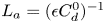 $L_a=(\epsilon C_{d}^0)^{-1}$ is the absorption length.
In order to obtain the absorption length, the divergence of the laser sheet, the direction of laser lines and the first pixels of laser path in the fluid are first calculated from the PLIF image of a dye solution of known concentration by marking on the edges of the shadow created by an opaque aperture in the path of the laser sheet by mouse clicks; in this step, the area of imaging and laser power was kept the same as that for the actual experiments. A fluorescence intensity image with a uniform concentration of dye equal to  $C_{d}^0$ is then recorded, and corrected for the background intensity variation and camera dark current by subtracting a dark image. Vignetting effects are then removed from the background-subtracted image by subtracting a white sheet image, obtained when the laser sheet grazes a vertical white sheet in its plane inside the test section. Since the direction of laser lines,
 $F$,
 $F_o$ and
 $x$ are known, (F 3) is fitted then through the fluorescence intensity data along each laser line to obtain its
 $L_a$.
A laser sheet of fixed power is then passed through various dye solutions of uniform, known concentrations, the obtained PLIF images are background and sheet corrected and then corrected for the absorption of light by the dye using the above calculated  $L_a$ to obtain uniform intensity images. The average light intensity from such images is then correlated with the uniform dye concentrations to obtain
 \begin{equation} C_{d} = (1.23\,F-7.14)\times 10^{-4}, \end{equation}
below a dye concentration of 0.48 p.p.m., where  $F$ is the fluorescence intensity expressed in intensity counts and
 $C_{d}$ is the concentration of the dye in p.p.m. The experimental PLIF images are background corrected, sheet corrected and absorption corrected and then the intensity distribution is converted to the dye concentration distribution using (F 4). We now need a relation to convert the dye concentration to the salt concentration, which is experiment specific; we obtain such a relation as follows.
The concentration of dye at any time instant  $C_{d}(x,y)$ in the experiments is converted into the concentration of salt
 $C_{e}(x,y)$ at the same time instant using
 \begin{equation} C_{e}(x,y)=A_1C_{d}(x,y)+A_2, \end{equation}
where  $A_1$ and
 $A_2$ are evaluated using the conditions in the top tank.
At the start of both the forcing and no-forcing experiments, under the well-mixed assumption, the concentrations of NaCl and the dye in the top tank satisfy,
 \begin{equation} \mathrm{at}\ t = 0: C_{e}(x,y)=C^0\quad \mathrm{and}\quad C_{d}(x,y)=0. \end{equation}
For the forcing experiments, at large times  $t_{\infty }$ after the start of the experiment, the concentration of NaCl and dye in the top tank are,
 \begin{equation} \mathrm{at}\ t = t_{\infty}: C_{e}(x,y)=0\quad \mathrm{and}\quad C_{d}(x,y)=C_{d}^0. \end{equation}
Substituting (F 6a,b) and (F 7a,b) in (F 5), we get
 \begin{equation} A_1=-\frac{C^0}{C_{d}^0} \quad \mathrm{and}\quad A_2=C^0. \end{equation}
Substituting these in (F 5), we obtain (F 5) at any time instant  $t$ as
 \begin{equation} \frac{C_e(x,y)}{C^0}=1-\frac{C_{d}(x,y)}{C_{d}^0}. \end{equation}
For the no-forcing experiments, at  $t=t_*$ when complete density equalisation of NaCl in the two tanks occurs,
 \begin{equation} \left.\begin{gathered} \mathrm{at}\ t = t_*: C_{e}(x,y)=C^0\frac{V_T}{V_T+V_B}\quad \mathrm{and}\\ C_{d}(x,y)=C_{d}^0\frac{V_B}{V_T+V_B}, \end{gathered}\right\} \end{equation}
Substituting (F 6a,b) and (F 10) in (F 5), results again in (F 8a,b). The dye concentration map obtained in experiments is converted into concentration maps of NaCl for both the forcing and no-forcing experiments by using (F 9), where  $C_{d}^0=0.48$ p.p.m is the concentration of the dye in the bottom tank before the start of the experiment.
Appendix G. Calculation of $C_{Be}(t)$

G.1. Estimation for no-forcing experiments
For the no-forcing experiments, we used both the conductivity probe as well as PLIF measurements to calculate  $C_{Be}(t)$, explained as follows. Note that the quantities measured by using the conductivity probe are given the subscript ‘
 $p$’. The concentration of NaCl in the top tank measured by the conductivity profile
 $(C_p(t))$ is calculated using the standard relation between conductivity and concentration of NaCl solution given in Lide (Reference Lide2003) under the well-mixed assumption (see Ramareddy & Puthenveettil Reference Ramareddy and Puthenveettil2011). An exponential decay fit between
 $C_p(t)$ and
 $t$ of the form,
 \begin{equation} C_p(t)=A_0+A_1\,\textrm{e}^{-t/d_1}+A_2\,\textrm{e}^{-t/d_2}+A_3\,\textrm{e}^{-t/d_3}+A_4\,\textrm{e}^{-t/d_4}, \end{equation}
where  $A_0$ to
 $A_4$ and
 $d_1$ to
 $d_4$ are the fit coefficients, is used for the calculation of
 $C_p$ at any time. The justification for choosing (G 1) with four exponential functions in the fit is given in Ramareddy & Puthenveettil (Reference Ramareddy and Puthenveettil2011).
For no-forcing experiments, since the total mass of NaCl at any instant is equal to the total mass of NaCl after density equalisation,
 \begin{equation} V_TC_p(t)+V_BC_{B}(t)=(V_T+V_B)\frac{C^0}{2}, \end{equation}
where  $C_{B}(t)$ is the instantaneous concentration of NaCl solution in the bottom tank and
 $V_T$ and
 $V_B$ are the volumes of liquid layers in the top and bottom tanks, respectively. Substituting for
 $C_{B}(t)$ from (G 2) in the expression for
 ${\rm \Delta} C_p(t)=C_p(t)-C_{B}(t)$, we get
 \begin{equation} {\rm \Delta} C_p(t)=\frac{V_T+V_B}{V_B}\left(C_p(t)-\frac{C^0}{2}\right). \end{equation}
In (G 2) and (G 3),  $C_p(t)$ is chosen to be
 $\langle C_e(y,t)\rangle$ at
 $y = 0.8$ mm, obtained from the PLIF images, and
 $C_{B}(t)$ calculated from (G 2) is used as
 $C_{Be}(t)$.
G.2. Estimation for forcing experiments
For the forcing experiments, the values of  $C_{Be}(t)$ are calculated entirely from the conductivity probe measurements, explained as follows. Let
 $t^0$ be the time of initiation of the experiment and
 $t_s$ the time from which the concentration changes monotonically after the initial mixing. To calculate
 $C_{Be}(t)$, i.e. the salt concentration in the bottom tank at any time after
 $t_s$, initially the salt concentration in the bottom tank at
 $t=t_s$ is first estimated using mass balance of the two tanks over the time interval
 $t=t^0$ to
 $t=t_s$ as
 \begin{equation} C_{Be}(t_s) = \frac{V_T}{V_B}(C^0-C_p(t_s)), \end{equation}
where  $C^0$ and
 $C_p(t_s)$ are obtained from the conductivity probe measurements. The mass balance in the bottom tank at any time
 $t$ is
 \begin{equation} \frac{\partial}{\partial t} \int_{\mathrm{CV}} C_{Be}(t)\,\mathrm{d}\forall\ = C_{Be}(t)V_iA_b, \end{equation}
where  $A_b$ is the cross-sectional area of the bottom tank. Integration and simplification of (G 5), using (G 4) gives
 \begin{equation} C_{Be}(t) = C_{Be}(t_s)\exp ((t_s-t)V_iA_b/V_B). \end{equation}
Since the concentration on the membrane cannot be measured from PLIF images, (G 6) is used to calculate  ${\rm \Delta} C_e(t)$ and then compared with (3.21).