A. Variability and Trends in Evapotranspiration and Precipitation: Global Is ≠ Regional

Climate change effects on the terrestrial water cycle show regional differentiated patterns. Although temperature is increasing in many world grape-growing regions (Hannah et al., Reference Hannah, Roehrdanz, Ikegami, Shepard, Shaw, Tabor, Zhi, Marquet and Hijmans2013; Jones et al., Reference Jones, Duchene, Tomasi, Yuste, Braslavska, Schultz and Martinez2005b; Schultz and Jones, Reference Schultz and Jones2010; Webb et al., Reference Webb, Whetton, Bhend, Darbyshire, Briggs and Barlow2012), precipitation patterns can differ vastly between regions and can show substantial temporal variations (between and within years; IPCC, 2014). From rising temperatures, it is mostly assumed that the water-holding capacity of the atmosphere will increase in the future as a function of the Clausius-Clapeyron law (Krysanova et al., Reference Krysanova, Buiteveld, Haase, Hattermann, van Niekerk, Roest, Martinez-Santos and Schlüter2008), which predicts an increase in the saturation vapor pressure of the atmosphere of 6%–7% per degree Celsius warming. As a consequence, a simultaneous increase in potential evapotranspiration (evaporation of water from the soil and transpiration of water from plants, ET₀) is assumed, which will alter soil and plant water relations. However, the large spatial and temporal variability in precipitation patterns between regions precludes generalizations in predicted consequences with respect to soil and plant water status development. Especially the temporal variability may mask longer-term trends in the development of ET₀ and consequently soil and plant water status (van Leeuwen, Pieri, and Vivin, Reference van Leeuwen, Pieri, Vivin, Delrot, Medrano, Or, Bavaresco and Grando2010; Gambetta, Reference Gambetta2016). Additionally, the focus on the developments within a growing season (spring to summer) in many studies may miss decisive effects occurring during the “off season” (winter to early spring) but having substantial carryover effects into the season.

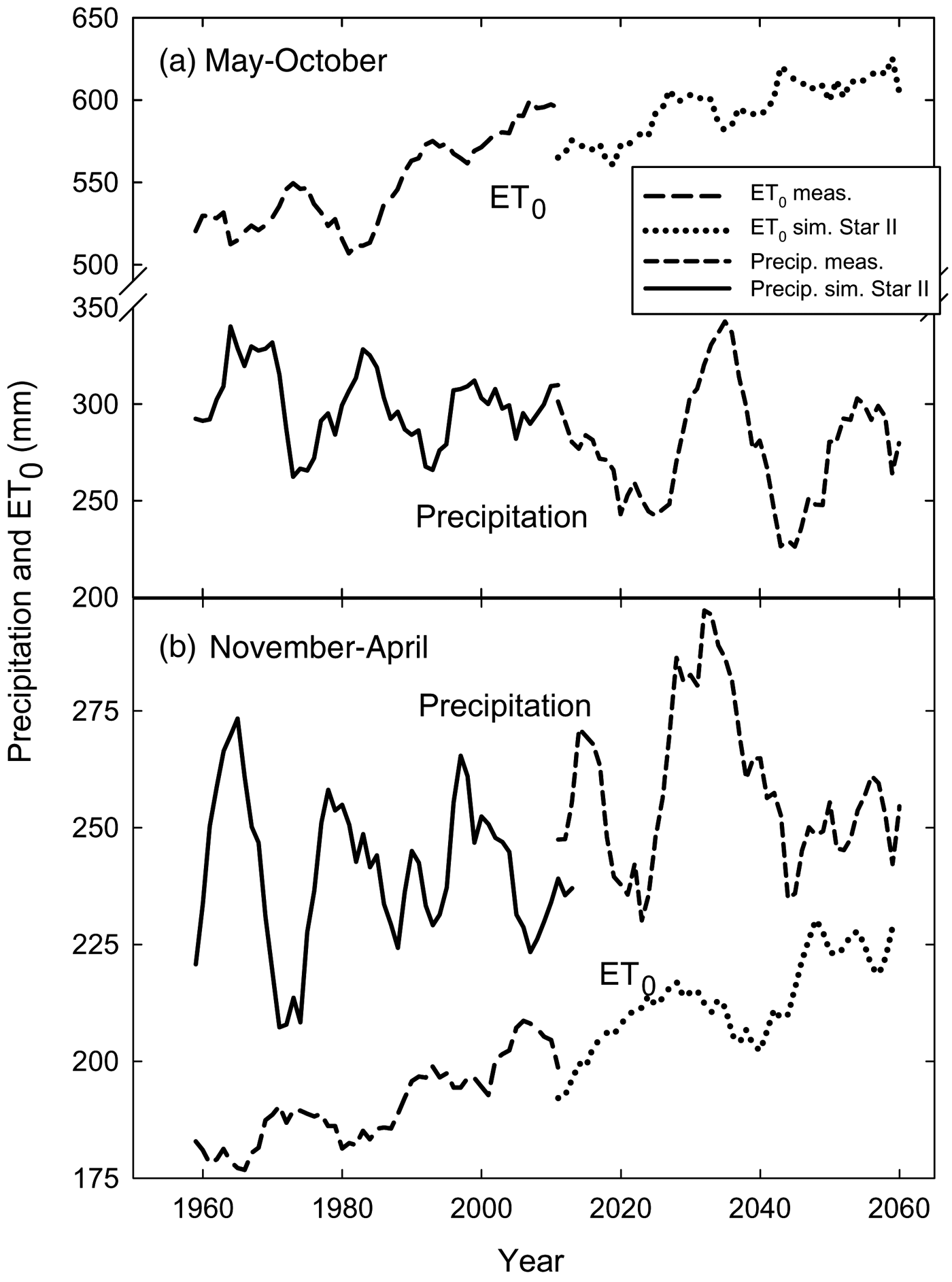
Figure 1 shows observed (calculated according to Penman-Monteith) and predicted changes in ET₀ during the growing season (May–October), which in agrometeorological terms is defined as the “hydrological summer” (Figure 1a), and the off season (November–April), which is the “hydrological winter” (Bormann, Reference Bormann2011) (Figure 1b) for the temperate wine-growing region of the Rheingau (Germany; 50.0° N, 8.0° E), from 1958 until 2060 (Schultz and Hofmann, Reference Schultz, Hofmann, Géros, Chaves, Medrano Gil and Delrot2015). To smooth out temporal variability, 10-year running mean values were used. There is a clear increase in the difference between ET₀ and precipitation rate during the growing season already observed during the past 55 years, and this development will continue in the future as predicted using a regionalized version of the STAR II model of the Potsdam Institute of Climate Impact Figure 1a; (Orlowsky et al., Reference Orlowsky, Gerstengarbe and Werner2008) (Figure 1a).

Figure 1

Observed and Simulated Precipitation and Potential Evapotranspiration (ET₀)

Notes: Observed and Simulated Precipitation and Potential Evapotranspiration for the hydrological summer (May–October) (a) and the hydrological winter (November–April) (b) for Geisenheim in the Rheingau grape-growing region (Germany, 50.0° N, 8.0° E; 92 m above sea level) (meas., measured; sim., simulated). Data show 10-year running mean values. Potential evapotranspiration rates for the observed time period (1958–2013) were calculated according to Penman-Monteith. Simulations were conducted with the STAR II model of the Potsdam Institute of Climate Impact using the medium realization run (Orlowsky, Gerstengarbe, and Werner, 2008). Source: Adapted from Schultz and Hofmann (2015).

Despite a “natural” focus on the developments within the growing season, changes in the water budget during the off season might also become very important (Figure 1b). Regardless of the fact that during winter and spring precipitation rates are exceeding ET₀, the “gap” between these two factors determining the soil water balance is decreasing and will be even more so in the future, irrespective of projected increases in precipitation rate (IPCC, 2014) (Figure 1b). This suggests that for this particular region winter precipitation will eventually be matched by winter ET₀ with important consequences for the amount of water stored in the soils at the beginning of the growing season. It may also have consequences for the use of cover crops during the winter.

Obvious from Figure 1 are the cyclic patterns of both potential evapotranspiration (ET₀) and precipitation rates, both for the period of observation and the projections until 2060. These cycles may be related to solar cycles, which have been made partly responsible for the warming during the first half of the last century but not during the second half (Stott et al., Reference Stott, Jones and Mitchell2003). However, there is some uncertainty on whether these cycles do continue to have an impact on the temporal development of warming on earth and consequently on evaporation (Stott et al., Reference Stott, Jones and Mitchell2003), but the data do show that variability and the development of extremes will become more likely despite cyclic variations (Figure 1; IPCC, 2014). These cycles have an important effect on how climate change is perceived by humans because these cycles can somewhat mask long-term trends (when precipitation is increasing or ET₀ is decreasing for several years) or on the contrary suggest a speedup in these trends (Figure 1).

Aside from Mediterranean-type, low summer rainfall climates with a more or less continuous decline in water availability over most of the growing season, temporary water deficits also commonly occur in temperate, summer rainfall regions, specifically on vineyard sites with shallow soils and low water-holding capacity (i.e., van Leeuwen, Pieri, and Vivin, Reference van Leeuwen, Pieri, Vivin, Delrot, Medrano, Or, Bavaresco and Grando2010). As compared with an irrigated vineyard situation in moderate or even hot climates, the natural cycles of stress and relief can be much more pronounced albeit completely unpredictable in frequency, duration, and severity in these areas and are naturally part of the “terroir” and the year-to-year variation in wine quality.

B. Air Temperature

It is difficult to draw clear relationships between climatology and vine performance or wine quality because obviously the ecophysiological adaptation and buffering capacity is large. How observed warming has impacted on yield formation is difficult to assess because cultivation practices, plant material, and production goals have changed substantially over the past 100 years, and there are only a few examples of a more extensive analysis on yield development (i.e., Bock et al., Reference Bock, Sparks, Estrella and Menzel2013; Lobell et al., Reference Lobell, Cahill and Field2007; Webb et al., Reference Webb, Whetton, Bhend, Darbyshire, Briggs and Barlow2012). The data of Bock et al. (Reference Bock, Sparks, Estrella and Menzel2013) from Germany go back to 1805 and suggest substantial yield increases since about 1910. There was a good correlation to temperature, but simultaneous developments in cultivation practices, plant protection measures, and in particular plant material have probably also played a substantial role. Less dramatic were observed yield effects over a much shorter time period in California (Lobell et al., Reference Lobell, Cahill and Field2007), and Webb et al. (Reference Webb, Whetton, Bhend, Darbyshire, Briggs and Barlow2012) reported decreasing yields for some regions in Australia in recent years, which may be more impacted by water availability than temperature. Water may actually be the decisive factor for positive or negative yield development in the future (Garcia de Cortazar Atauri, Reference Garcia de Cortazar Atauri2006).

Certainly, climatic variables affect grape composition, as evidenced by long-term increases in temperature in the past being implicated in altered fruit composition (mainly increase in sugar concentration and a decrease in acidity) in Europe, North America, and Australia (Duchêne and Schneider, Reference Duchêne and Schneider2005; Petrie and Sadras, Reference Petrie and Sadras2008; Schultz, Reference Schultz2000; Schultz and Jones, Reference Schultz and Jones2010; Urhausen et al., Reference Urhausen, Brienen, Kapala and Simmer2011; Webb et al., Reference Webb, Whetton, Bhend, Darbyshire, Briggs and Barlow2012; Wolfe et al., Reference Wolfe, Schwartz, Lakso, Otsuki, Pool and Shaulis2005); however, there may be counteracting effects if different regions with a different climatic matrix are compared. In some cases, changes in cultivation practices and consumer demand may have contributed more to the increase in sugar concentration at harvest than changes in the climate (Alston et al., Reference Alston, Fuller, Lapsley and Soleas2011). Although many studies have used temperature summations to predict shifts in the varietal spectrum (i.e., Hannah et al., Reference Hannah, Roehrdanz, Ikegami, Shepard, Shaw, Tabor, Zhi, Marquet and Hijmans2013; Kenny and Harrison, Reference Kenny and Harrison1992), these approaches do not incorporate factors such as day–night variations, sunshine hours, or water availability, which are cofactors in quality formation, and they additionally neglect possible mitigation strategies through cultivation methods. Using upper temperature thresholds (which are not really known) to predict varietal shifts (Hannah et al., Reference Hannah, Roehrdanz, Ikegami, Shepard, Shaw, Tabor, Zhi, Marquet and Hijmans2013) may result in erroneous scenarios (van Leeuwen et al., Reference van Leeuwen, Schultz, Garcia de Cortazar-Atauri, Duchêne, Ollat, Pieri and Bois2013).

Different varieties will respond differently to warming. For example, an increase in temperature from 20 °C to 30 °C increased the weight of bunch primordia (preformed inflorescences in the latent winter buds) fourfold in Riesling, but Shiraz was unaffected (Dunn, Reference Dunn, de Garis, Dundon, Johnstone and Partridge2005). Shiraz also showed very little response in basic yield components in a 2 °C to 4 °C warming experiment (Sadras and Soar, Reference Sadras and Soar2009). In principle, red varieties appear to tolerate warm conditions better than white varieties. Sadras et al. (Reference Sadras, Stevens, Pech, Taylor, Nicholas and McCarthy2007) found contrasting responses for red and white varieties across 24 Australian wine regions. There was a positive correlation of quality ratings and daily mean regional temperature for red but not for white wines, whereas the apparent influence of temperature on vintage variability was strong for white wines but irrelevant for red wines. However, when wine score data were correlated with the average growing season temperature (October to April), there was a negative trend for red and white wines in some of the analyzed regions (Hayman et al., Reference Hayman, McCarthy, Soar, Sadras, Sadras, Soar, Hayman and McCarthy2009).

When sensory traits of berries from different varieties were compared in a warming study, a clear distinction between red and white varieties was not apparent. Moreover, a white variety such as Chardonnay responded favorably to an increase in temperature (Sadras, Moran, and Bonada, Reference Sadras, Moran and Bonada2013). Jones et al. (Reference Jones, White, Cooper and Storchmann2005a) analyzed the vintage ratings of Sotheby's from all major wine regions worldwide between 1950 and 1999 and found that most quality ratings were improved, but that there might be some temperature thresholds that would cause a decline in quality.

Heat waves may also trigger quite diverse responses in terms of grape composition. Pillet et al. (Reference Pillet, Egert, Pieri, Lecourieux, Kappel, Charon, Gomès, Keller, Delrot and Lecourieux2012) showed that the raffinose oligosaccharide pathway was activated in grape berries after simulated heat stress leading to the formation of galactinol from sucrose, yet we do not know if this has any sensory impact on wine.

The economic consequences of climate change for the wine industry on a global scale are difficult to predict because variability between regions is large and the process of change is nonlinear (example given in Figure 1) (Ashenfelter and Storchmann, Reference Ashenfelter and Storchmann2016). For example, Ashenfelter and Storchmann (Reference Ashenfelter and Storchmann2010) tried to model the effects of climate change on the quality, prices, and land value in the Mosel Valley based on solar radiation but from an economist's viewpoint. They concluded that an increase in temperature will increase quality as well as price and land value, thus corroborating, for the quality aspect, the analysis by Jones et al. (Reference Jones, White, Cooper and Storchmann2005a). However, comparing past quality ratings with temperature (as in Jones et al., Reference Jones, White, Cooper and Storchmann2005a) and modeling the future require quite different hypotheses, and the underlying assumptions in the study by Ashenfelter and Storchmann (Reference Ashenfelter and Storchmann2010) seem too simplistic in some cases. For example, deeper soils were rated of lesser importance for quality, but for white wines, water-holding capacity is a key factor in aroma formation (contrary to red wines). Thiol concentration, an important flavor group for Riesling and Sauvignon blanc, is reduced by water deficit (Peyrot des Gachons et al., Reference Peyrot des Gachons, Van Leeuwen, Tominaga, Soyer, Gaudillère and Dubourdieu2005; Schüttler et al., Reference Schüttler, Gruber, Thibon, Lafontaine, Stoll, Schultz, Rauhut and Darriet2011), and 1,1,6-Trimethyl-1,2-dihydronaphtalene (TDN), the compound responsible for petrol flavors in wines produced from Riesling grapes (main variety in the Mosel Valley), increases with temperature during the berry-ripening phase (Marais, van Wyk, and Rapp, Reference Marais, van Wyk and Rapp1992) but is rated negative for wine quality. Additionally, steep slopes, which are favored in this analysis, not only have higher incoming solar radiation but also show, as a result of this, much higher evapotranspiration rates, which for a slope of 30° results in an increase of water use of approximately 25% (Hofmann, Lux, and Schultz, Reference Hofmann, Lux and Schultz2014). This had positive effects in the past, where ET₀ rates were lower (see Figure 1) to avoid a surplus of water, specifically during the ripening phase when sloping effects are largest (Hoppmann, Reference Hoppmann2010). However, a future climate may have exactly the opposite impact. Ashenfelter and Storchmann (Reference Ashenfelter and Storchmann2010) also penalized a greater altitude difference between the river and the vineyard in question in terms of quality due to an increase in day–night temperature amplitude. There is no clear scientific basis for such an assumption, because cool nights reduce carbon use by respiration and thus retain the carbon pool as molecular background for aroma and color formation (Pirie and Mullins, Reference Pirie and Mullins1980) and the “cool night index” is part of the classification of positive climate criteria for the evaluation of wine regions (Tonietto and Carbonneau, Reference Tonietto and Carbonneau2004). However, altitude may have a negative effect on photosynthesis (due to lower day temperatures) as long as day temperatures are near the lower limit of the optimum (Schultz, Reference Schultz2000). Other analyses came to a completely different conclusion, albeit for a generally much warmer environment. White et al. (Reference White, Diffenbaugh, Jones, Pal and Giorgi2006) predicted a decrease in “premium wine production” of 81% by the end of the current century for the U.S. wine regions due to the projected increases in temperature, and Hannah et al. (Reference Hannah, Roehrdanz, Ikegami, Shepard, Shaw, Tabor, Zhi, Marquet and Hijmans2013) suggested that many classical wine-growing regions will lose a large percentage of their grape-producing vineyards due to the combined effects of temperature and water deficit. This is in agreement with the general conclusion of Ashenfelter and Storchmann (Reference Ashenfelter and Storchmann2016) that increased warming may increase the number of good vintages in cold climate wine regions and simultaneously decrease the number of good vintages in hot climate growing regions, but the thresholds are difficult to define.

Figure 2

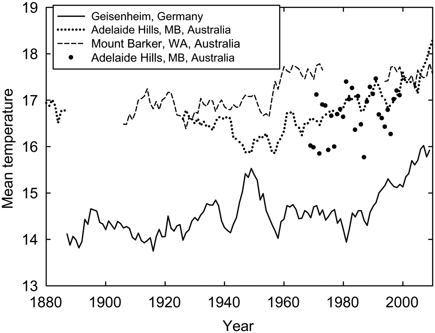
Temperature Development during the Growing Season (Average Temperature April–October, Northern Hemisphere; October–April, Southern Hemisphere) for Three Grape-Growing Regions with a Reputation for High-Quality Riesling Wines

Sources: The data are 5-year running mean values for Geisenheim in the Rheingau region, Germany (50.0° N, 8.0° E; altitude 92 m above sea level [a.s.l.]), from the Deutsche Wetterdienst (German Weather Service) database. The data for the Australian regions, Mount Barker (MB), Western Australia (WA; −34.6° S, 117.6° E; altitude 300 m a.s.l.), and Adelaide Hills (−35.1° S, 138.8° E; altitude 360 m a.s.l.), are from the Commonwealth of Australia, Bureau of Meteorology. Additional available data are shown for Lenswood (1967–1999), a classical Riesling area in the Adelaide Hills that does not have a long historic weather record but is situated at a higher altitude (480 m), to show the similarity with the long-term records from the weather station at lower altitude.

Basically, the underlying assumptions about the suitability of a certain climate for grapevine cultivation, or more precisely the cultivation of different varieties, are decisive for the outcome. These assumptions have been partly based on erroneous criteria about the suitability of different varieties under certain temperature scenarios. We do know the lower limit in growing season temperature for many grape varieties (e.g., Huglin, Reference Huglin1978; Jones, Reference Jones, Macqueen and Meinert2006), but we do not know the upper limit. Both the temperature summation index of Huglin (Reference Huglin1978) and the figure published by Jones (Reference Jones, Macqueen and Meinert2006) on the suitability of grapevine varieties as a function of temperature have been misused to predict the “nonsuitability” of a particular variety when growing season temperatures (in future climate scenarios) exceed the given values of the current production areas (e.g. Hannah et al., Reference Hannah, Roehrdanz, Ikegami, Shepard, Shaw, Tabor, Zhi, Marquet and Hijmans2013). In terms of quality and suitability, van Leeuwen et al. (Reference van Leeuwen, Schultz, Garcia de Cortazar-Atauri, Duchêne, Ollat, Pieri and Bois2013) have clearly demonstrated that growing season temperatures in this century have already surpassed the presumed upper limit of suitability in Jones (Reference Jones, Macqueen and Meinert2006) for key varieties in the Rheingau (Germany), Burgundy (France), and Rhone (France) grape-growing regions without detrimental effects on quality.

Figure 2 shows an example for the growing season temperature development (average temperature between April and October for the Northern Hemisphere and between October and April for the Southern Hemisphere) over the past 130 years for three grape-growing regions with a reputation for the variety Riesling, one in the Northern Hemisphere (Rheingau, Germany) and two in the Southern Hemisphere (Mount Barker, Western Australia, and Adelaide Hills, South Australia). Because long-term weather data are not always available from stations directly within grape-growing regions, additional data from Lenswood, a known Riesling area in the Adelaide Hills, are added for the available period from 1967 to 1999 to show the similarity with the other chosen Adelaide Hills station. It is obvious that despite growing the same variety, average temperatures during the season show substantial differences between all three grape-growing regions and that the Australian regions have surpassed the 17 °C threshold of Riesling suitability given in the Jones (Reference Jones, Macqueen and Meinert2006) chart for the past 20 years. The key factor is our missing knowledge of varietal plasticity with respect to environmental variables (Sadras et al., Reference Sadras, Schultz, Girona, Marsal, Steduto, Hsiao, Fereres and Raes2012) and the lack of capacity to integrate the effects of these factors on fruit composition and subsequently on wine quality. The warming trend in general was more dominated by increases in night than day temperatures confirming observations from other areas (Nemani et al., Reference Nemani, White, Cayan, Jones, Running, Coughlan and Peterson2001), but the degree of change was highly dependent on the month in question (data not shown).

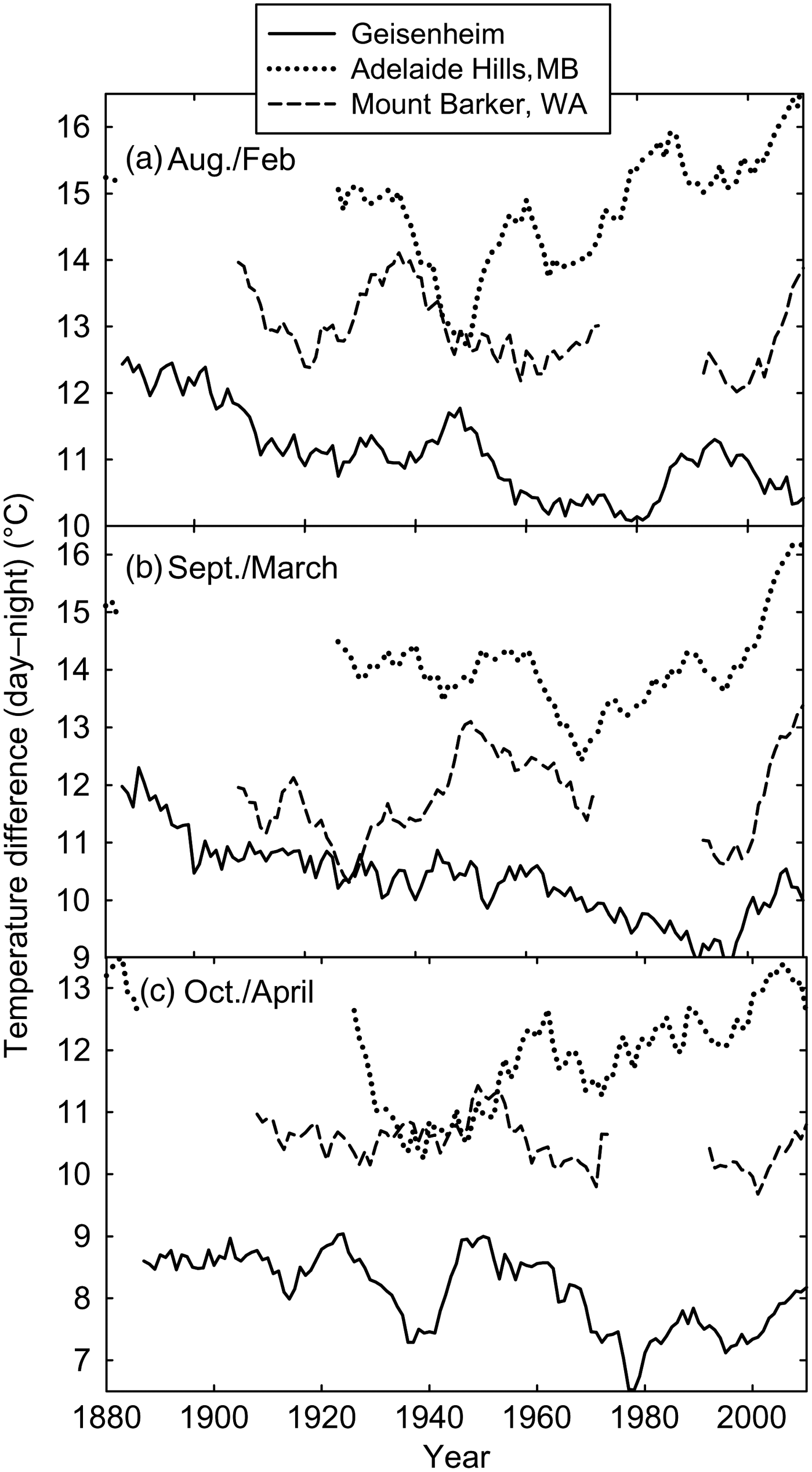
To extend the given example of a cross-regional comparison, Figure 3 shows the day–night temperature amplitude of the same German and Australian “Riesling” areas during the 3 months relevant for berry ripening (August to October for the Northern Hemisphere and February to April for the Southern Hemisphere). It is clear that cross-regional differences are large and also that climatic trends seem to be different with respect to this environmental parameter over the past 130 years. Day–night temperature difference is largest in the Adelaide Hills, between 13 °C to 16 °C in February and March (equivalent to August and September in the Northern Hemisphere), as compared with Geisenheim, where day–night differences are between 9 °C and 12 °C (Figure 3a and 3b). Additionally, it seems that the daily temperature amplitude has more or less continuously decreased in Geisenheim, whereas the Southern Hemisphere data suggest a larger variability and also a trend to an increase in amplitude during the past 30 to 40 years (Figure 3).

Figure 3

Development of Day–Night Temperature Differences for the 3 Months Relevant for Ripening (August–October, Northern Hemisphere; February–April, Southern Hemisphere) for Three Grape-Growing Regions with a Reputation for High-Quality Riesling Wines in Germany and Australia

Note: For additional information on sites, see Figure 2. Sources: The data are 10-year running mean values for Geisenheim based on data provided by the Deutsche Wetterdienst (German Weather Service). The data for the Australian regions are from the Commonwealth of Australia, Bureau of Meteorology.

It seems logical that the “flavor shape” of wines from different regions will be different (Iland et al., Reference Iland, Dry, Proffitt and Tyerman2011) given that enzyme activity in the fruit is related to temperature. Kliewer and Torres (Reference Kliewer and Torres1972) showed that an increase in day–night temperature difference may improve coloration for red grapes as long as daily maximum temperatures are not too high, and Hale and Buttrose (Reference Hale and Buttrose1974) confirmed these findings. It seems possible, however, that conditions such as warmer days and cooler nights (thus higher day–night temperature differences) have a similar effect as cooler days and warmer nights (thus lower day–night temperatures) as long as the time periods within the optimum range are similar, yet we are lacking data on this for white grapes (Haymann et al., Reference Hayman, McCarthy, Soar, Sadras, Sadras, Soar, Hayman and McCarthy2009; Winter, Lowe, and Bulleid, Reference Winter, Lowe and Bulleid2007).

Several studies have shown that grapevine phenology has significantly advanced in many wine-growing regions in the past as a response to warming trends such as those shown in Figure 2 (i.e., Duchêne and Schneider, Reference Duchêne and Schneider2005; Jones et al., Reference Jones, Duchene, Tomasi, Yuste, Braslavska, Schultz and Martinez2005b) and will continue to shift forward in time with the main ripening period occurring at much higher temperatures (Webb, Whetton, and Barlow, Reference Webb, Whetton and Barlow2007). It is also clear that the changes that occurred over the past 130 years within each region were not larger in magnitude than the existing differences between these regions (Figures 2 and 3). Because they all grow the same variety, there seems to be a significant potential for acclimation and plasticity (Sadras et al., Reference Sadras, Stevens, Pech, Taylor, Nicholas and McCarthy2007), which would have to be included in any economic analysis and “speculation” on varietal suitability and thus sustainability in the future.

C. Soil Temperature

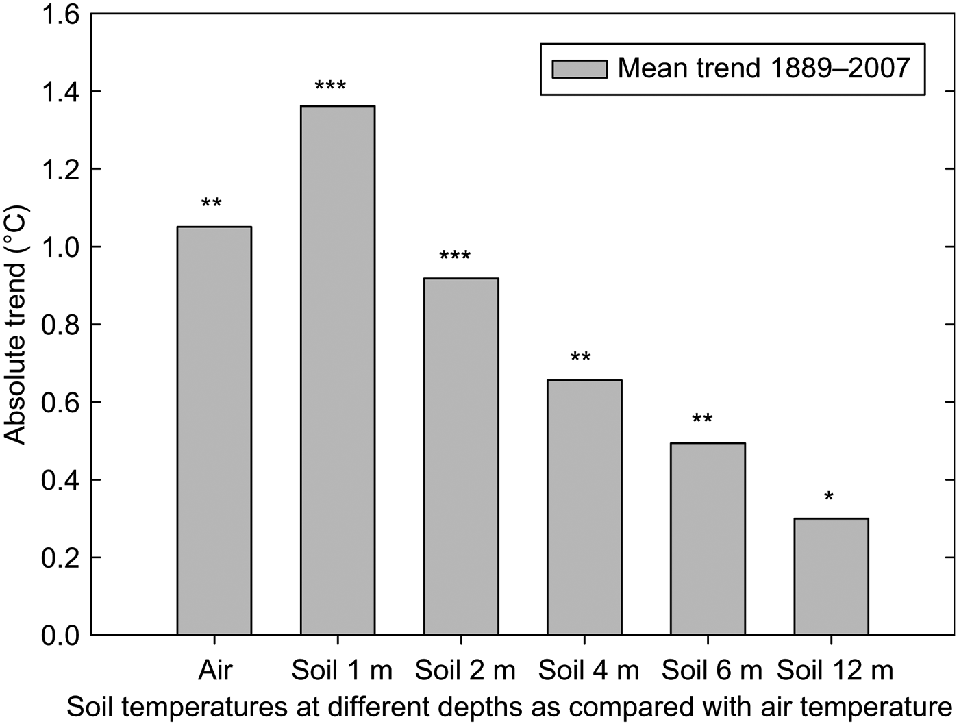
Soil temperature has increased at least at a rate similar to air temperature over the past more than 100 years (Figure 4; Böhme and Böttcher, Reference Böhme and Böttcher2011). A relatively unique time series of soil temperatures down to 12 m depth since 1889 reveals that soil temperatures in the upper 1 m profile have increased by approximately 2 °C to 3 °C between April and August as compared with the beginning of data collection (Böhme and Böttcher, Reference Böhme and Böttcher2011). Higher temperature in combination with an increased propensity yet variable spatial distribution of heavy rainfall events (Feldmann et al., Reference Feldmann, Schädler, Panitz and Kottmeier2013) seems to have already increased the risk for the development of rot (Botrytis cinerea) in some areas and will most likely continue to do so.

Figure 4

Observed Trends in Soil Temperature at Different Soil Depths between 1889 and 2007 at Potsdam, Germany as Compared to Air Temperature

Notes: Measurements were conducted continuously with the same techniques. Asterisks indicate different levels of significance over eleven 10-year periods (***1%, **10%, *20%). Source: Adapted from Böhme and Böttcher (2011).

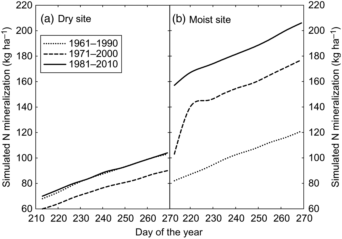
When the patterns in temperature and precipitation during the grape-ripening phase over the period from 1955 to 2014 for the Rheingau area are analyzed, it becomes clear that 14 of the last 15 vintages had a warmer maturation period than the median over the 59 years in question and that 10 of these vintages had average and above-average precipitation rates during berry maturation and only 4 were drier than the median. This indicates the increased risk for the development of B. cinerea in recent years, which can also be quantified using a soil nitrogen (N) model, capable of simulating the mineralization rates of different soil types depending on soil characteristics (i.e., organic matter content, water-holding capacity, pore size distribution, etc.), precipitation rates, and other climate variables such as air temperature and solar radiation (Schaller et al., Reference Schaller, Jagoutz, Berthold, Emde, Lohnertz and Hoppmann1994a, Reference Schaller, Jagoutz, Berthold, Emde, Lohnertz and Hoppmann1994b). Comparing the simulated rates of N mineralization during the growing season for 30-year periods since 1961 shows increasing rates over the past 50 years with substantial differences between soils (Figure 5). This analysis suggests that modifications in temperature and water relations in some vineyard sites have already had a substantial impact on the release of N, which might have increased the risk for bunch rot development on these sites already. Nevertheless, a recent study on warming effects on microbial communities in temperate vineyard soils, which would be involved in N mineralization, did not find substantial changes (Corneo et al., Reference Corneo, Pellegrini, Cappellin, Gessler and Pertot2014).

Figure 5

Simulated Cumulative Maximum Nitrogen (N) Mineralization over the Season

Notes: Using an “average year” (mean of 30 years) for the periods 1961–1990, 1971–2000, and 1981–2010 for two vineyard sites with soils with average organic matter content for Geisenheim, Germany. Results for a dry sandy/loam soil (a) and for a clay soil with good water-holding capacity (b). Simulations were conducted with a model developed by Schaller et al. (1994a, 1994b).

D. CO₂ Concentration

Aside from the fact that increasing CO₂ concentrations will impact on global temperature, CO₂ itself is generally beneficial to plant growth, although the response strongly varies between species (Long et al., Reference Long, Ainsworth, Rogers and Ort2004). For grapes, the increase in CO₂ concentration has been calculated to have a significant positive effect on yield (Adams, Wu, and Houston, Reference Adams, Wu and Houston2003). Because stomata are sensitive to CO₂ but photosynthesis increases in response to it, increased biomass production at reduced water losses is expected (Long et al., Reference Long, Ainsworth, Rogers and Ort2004), but a concomitant rise in temperature may still increase the water use of many crops (Adams, Wu, and Houston, Reference Adams, Wu and Houston2003). The concomitant rise in water-use efficiency may be exacerbated depending on the degree of stomatal closure and considering that the respiration rate may also be suppressed by elevated CO₂ (eCO₂). However, studies on individual leaves may not be representative of whole plant field experiments, and the need to study the effects of eCO₂ and temperature in combination is necessary albeit experimentally challenging. Despite a pressing need to gain more information, CO₂ responses beyond those of the photosynthetic apparatus and associated physiology and metabolism such as quality aspects of agricultural commodities have only attracted limited attention (Feng, Li, and Cheng, Reference Feng, Li and Cheng2014), yet the necessity for an increase in global food production and the high added-value potential specifically for special crops (horticultural products including grapes and wine) warrants a closer look at their CO₂ response profile.

Few studies have investigated the response of grapevines to CO₂ outdoors, either in small free air CO₂ enrichment systems (Bindi et al., Reference Bindi, Fibbi, Gozzini, Orlandini, Miglietta, Harrison, Butterfield and Downing1995; Bindi et al., Reference Bindi, Fibbi, Lanini and Miglietta2001) or in open-top chambers (Gonçalves et al., Reference Gonçalves, Falco, Moutinho-Pereira, Bacelar, Peixoto and Correia2009), but these could only describe the impact of eCO₂ concentration in the absence of rising air temperature. Nevertheless, the generally predicted increase in biomass was confirmed, yet the effects on water consumption remained unclear (Bindi et al., Reference Bindi, Fibbi, Gozzini, Orlandini, Miglietta, Harrison, Butterfield and Downing1995; Bindi et al., Reference Bindi, Fibbi, Lanini and Miglietta2001). These experiments also showed that fruit sugar concentration should increase and acidity levels decrease under eCO₂ (Bindi, Fibbi, and Miglietta, Reference Bindi, Fibbi and Miglietta2001); however, the response of other components contributing to the flavor and aroma of grapes was heterogeneous and indicated a significant “chamber effect,” with plants grown outside responding differently than plants in open-top chambers with or without eCO₂ (Gonçalves et al., Reference Gonçalves, Falco, Moutinho-Pereira, Bacelar, Peixoto and Correia2009).

A more recent series of studies investigated the effects of shorter-term exposures to eCO₂ (700 ppm) in combination with changes in the temperature and water regime on small potted plants in a greenhouse (Salazar-Parra et al., Reference Salazar-Parra, Aguirreolea, Sánchez-Díaz, Irigoyen and Morales2010, Reference Salazar-Parra, Aguirreolea, Sánchez-Díaz, Irigoyen and Morales2012a, Reference Salazar-Parra, Aguirreolea, Sánchez-Díaz, Irigoyen and Morales2012b). Similar to the results of Bindi, Fibbi, and Miglietta (Reference Bindi, Fibbi, Lanini and Miglietta2001), eCO₂ decreased malic acid and, in combination with elevated temperature, also total anthocyanins in well-watered plants (Salazar-Parra et al., Reference Salazar-Parra, Aguirreolea, Sánchez-Díaz, Irigoyen and Morales2010) and caused less oxidative damage under water deficit (Salazar-Parra et al., Reference Salazar-Parra, Aguirreolea, Sánchez-Díaz, Irigoyen and Morales2012a), yet expected differences in photosynthetic rate disappeared with time under eCO₂ (Salazar-Parra et al., Reference Salazar-Parra, Aguirreolea, Sánchez-Díaz, Irigoyen and Morales2012b). It currently remains unknown how long-term exposure to eCO₂ (i.e., years) would affect grapevines as perennial plants.

Another area, which needs to receive more attention, is the effect of global warming and increase in ambient CO₂ concentration on plant–pathogen interactions. Recent results have shown that these interactions can be modified and could lead to an increase in insect aggressiveness (DeLucia et al., Reference DeLucia, Casteel, Nabity and O'Neill2008), population biology, and the sequence of potential epidemics (Garrett et al., Reference Garrett, Dendy, Frank, Rouse and Travers2006). The basis for these modifications lies within the potential modification of the genome of microorganisms and/or insect pathogens or the expression patterns of genes (Travers et al., Reference Travers, Smith, Bai, Hulbert, Leach, Schnable and Knapp2007). Thus, there is a potential threat to agricultural productions systems that goes well beyond the mere spread of diseases into areas where these have not been known previously due to global warming.

E. Nitrous Oxide, Methane, and the Carbon Budget of Vineyards

An additional challenge will be the largely missing information about how much viticultural production systems contribute to the release of nitrous oxide and methane, two of the most potent greenhouse gases (Carlisle et al., Reference Carlisle, Smart, Williams and Summer2010), or how these systems could be adapted to become less of a source for these gases or even a sink (at least for methane that seems a possibility; Dalal et al., Reference Dalal, Wang, Robertson and Parton2003). Equally largely unknown are strategies to improve the carbon budget of vineyards, so far in most cases not included in carbon budget protocols (Carlisle, Steenwerth, and Smart, Reference Carlisle, Steenwerth and Smart2006). These topics require long-term research strategies, and the importance of beginning to gather information has been realized in some grape-growing areas such as California (Carlisle et al., Reference Carlisle, Smart, Williams and Summer2010; Steenwerth and Belina, Reference Steenwerth and Belina2008). To elucidate the complex interactions between compounds and management will be a challenging task, but results are urgently needed. Carlisle et al. (Reference Carlisle, Smart, Williams and Summer2010) have formulated research goals in particular with respect to the following:

1. 1. Factors relating to the production of nitrous oxide, such as N leaching/volatilization; fertilization amount, timing, and method; and the interactions with management practices (including irrigation).

2. 2. Factors relating to vineyard carbon sequestration such as vine biomass, cover crop biomass, and soil carbon storage capacity, because this information is absent from carbon budget protocols in the wine sector.

3. 3. Factors relating to vineyard short- to medium-term floor management such as cover crops and tillage.

4. 4. Factors relating to vineyard long-term management effects on carbon sequestration and the interactions with other greenhouse gas emissions.

5. 5. Factors relating to methane production and uptake.

F. Carbon and Water Footprint of the Wine Industry

An additional challenge for the wine industry is more related to the management of natural resources in the production chain for wine and the resulting carbon or water footprints. Whereas the carbon footprint for entire regions has been roughly estimated (examples for the Champagne and Bordeaux regions) and some strategies devised to reduce it, the water footprint is an issue that will affect agriculture in general. Water management is no longer an issue restricted to individual countries or river basins. Even a continental approach is not sufficient. The water footprint of Europe—the total volume of water used for producing all commodities consumed by European citizens—for example has been significantly externalized to other parts of the world (Hoekstra and Chapagain, Reference Hoekstra and Chapagain2008). Rising food demand and growing water scarcity (IPPC, 2014) will put increasing pressure on agriculture, which is currently using up approximately 70% of the world's freshwater resources.

Currently, issues such as the amount of water imported by a country through products (including the direct input of water used for its production and the indirect water used for services around this product [transport or packaging]) are emerging in the context of water-neutral production budgets of countries or sustainability strategies of supermarket chains. Spain, for instance, is exporting 189 million m³ of water per year to the United Kingdom alone captured in products related to grape production (Chapagain and Orr, Reference Chapagain and Orr2008). These calculations and budgets are beginning to have impacts on production strategies in the wine industry, with the first signs appearing in California and Australia. Additionally, the water issue cannot be seen as strictly independent from other climate-related problems, because the release of nitric oxide and CO₂ from agricultural land contributes significantly to the “greenhouse effect,” and because this release depends on soil water content, irrigation management, and organic matter content (Avrahami and Bohannan, Reference Avrahami and Bohannan2009). For grape production, however, we have currently only very limited information on the contribution and/or possible management strategies of these effects, another significant challenge for future research (Herath et al., Reference Herath, Green, Singh, Horne, van der Zijpp and Clothier2013; Lamastra et al., Reference Lamastra, Suciu, Novelli and Trevisan2014).