1. Introduction

As the only terrestrial link between the main part of Antarctica and temperate latitudes, the Antarctic Peninsula is a key area for detection of north-south shifts of south-polar boundaries in the atmosphere and ocean that could be discovered through ice coring (Reference Peel,, Mulvaney,, Pasteur,, Chenery, Jones,, Bradley, and Jouzel,Peel and others, 1996). Recent shallow and intermediate depth cores from the Dyer Plateau (Fig. 1) have given a high-resolution history of glacio-climate over the last 480 years for this location (Reference Thompson,Thompson and others, 1994). The deepest core to date was collected in 1990 from a local dome on the divide at 70° 40.16 ′ S, 64° 52.30 ′ W. The core depth (≈ 235 m) was 64% of the total ice thickness at the site (≈ 365 m). In this paper we examine the dynamic conditions of the ice in this region of the Dyer Plateau relevant to the 1990 core and possible future cores that could extend the record of climate.

Fig. 1.

Location of the Dyer Plateau. Arrow tip indicates the site of measurements.

The principal dynamic information is the geometry of the ice, the strain rate on the upper surface and vertical strain rate along the core hole. These data are used to analyze the depth distributions of density and annual layer thicknesses measured in the core (Reference Thompson,Thompson and others, 1994) with the goals of estimating the current rate of thickness and mass change and refining information on the history of accumulation.

2. Geometry and Surface Motion

Geometry of the ice sheet was determined by measurements in a grid of markers on the upper surface (Fig. 2). The relative position of grid markers in a local coordinate system was determined by redundant angle (theodolite) and slope distance (electronic distance meter) measurements reduced by least-squares network adjustment. (The adjustment program was developed by L. A. Rasmussen and E. D. Waddington (unpublished information)). Errors estimated on the basis of residuals in the adjustment were typically within 0.03 m in the horizontal and 0.1 m in the vertical for the central part of the grid, but larger errors up to 0.7 m are indicated for a few markers on the distant edges of the grid, (See Reference Raymond,, Weertman and Mulvancy,Raymond and others (unpublished) for detailed compilation of survey data and results of net reduction.)

Fig. 2.

Spatial arrangement of surface observations. Points show location of poles used as markers. Thick, shaded lines show paths of radio-echo sounding traverses. Contours show surface elevation with a 5 m contour interval, as determined by survey of the markers interpolated by barometric altimetry along the traverses. Absolute elevation was based on positioning using transit satellites of a marker at the local summit. The horizontal axis of the figure is oriented 8.3° east of north (347.5° magnetic). Bars show the direction and speed of horizontal motion.

The grid was surveyed in 1990 and 1992, and relative displacements were computed for the 2 year interval. To remove indeterminacy associated with rigid translation and rotation, it was assumed that horizontal displacement at the local summit was zero and that markers on the divide north of this summit moved parallel to the divide. Absolute positions determined for four markers using observations from transit satellite (Magnavox Geoceiver 1502) were consistent with these assumptions, but were insufficiently accurate to control usefully the absolute displacements over the 2 year interval because of the generally slow speeds.

Grid lines were traversed with a radio-echo sounder (RES) to determine ice thickness and depth to internal reflectors (Reference Weertman,Weertman, 1993). The RES recorded barometric pressure, which allowed interpolation of elevation between surveyed grid markers.

The combined survey results were used to derive the surface elevation and velocity pattern (Fig. 2) and bed topography (Fig. 3). The geometry is characterized by a relatively smooth surface with a topographic divide running approximately north—south that is underlain by a complex of peaks and ridges. The relief on the bed within the grid is about 0.8 km, which is similar to the mean ice thickness. Horizontal speed on the surface increases with distance on either side of the divide, reaching about 5 ma ⁻¹ at 10 km from the divide.

Fig. 3.

Topography of the ice-sheet base. Contours show bed elevation with a 50 m contour interval. Thick, shaded lines show paths of radio-echo sounding traverses along which thickness was measured using two-way travel times to bed reflections (Reference Weertman,Weertman, 1993).

The 1990 core site was located near the summit of the north—south divide (Fig. 2). This summit lies over a sharp east—west trending ridge in the bed terrain (Fig. 3). It is one of the shallowest locations in the region. Thickness at this location is (365 ± 8) m.

Horizontal velocity divergence ė_d is of order 10⁻³ a⁻¹ in the vicinity of the summit. At the 1990 core site, principal horizontal strain rates ate ė₁ = (1.4 ± 0.1) × 10⁻³ a⁻¹ with azimuth 249°, and ė₂ = (0.5 ± 0.1) × 10⁻³ a⁻¹ with azimuth 159°, where azimuths are given east of true north. The total horizontal velocity divergence is ė_d = ė₁ + ė₂ = (1.9 ± 0.1) × 10⁻³ a⁻¹. Horizontal velocity at the core site is not accurately known from measurements. It is assumed to be less than 0.3 m a⁻¹, based on the distance from the summit to the site (< 200 m) and the strain rate along the slope (< 0.0015 a⁻¹).

3. Surface Conditions

Surface snow density was measured from the core and in pits. Average density in the meter just beneath the surface was 420 kg m⁻³. The 10 m temperature at the core site is −21°С (Reference Thompson,Thompson and others, 1994).

Rate of snow accumulation over a 2–3 year interval was determined by measurements of snow-height change on poles in the network (Fig. 2). Snow settlement was taken into account based on the near-surface density profile and the assumption that the bases of poles moved with the local snow. The average accumulation rate measured on eight poles within 0.5 km of the 1990 summit core site is 1.17 m a⁻¹ with a standard deviation of ±0.10 m a⁻¹. If it is assumed that the scatter in measurements arises from uncorrelated errors or Spatial variation, then the standard error of the average is 0.05 m a⁻¹. When corrected for density, the average snow accumulation rate gives a surface mass-balance rate of 490 kg m⁻² a⁻¹ (0.49 m a⁻¹ water-equivalent thickness, 0.54 m a ⁻¹ ice-equivalent thickness).

The spatial pattern of accumulation rate over the full grid was examined using a combination of measurements on the poles of the grid and the depth of near-surface horizons detected by radar (Reference Weertman,Weertman, 1993; paper in preparation by B.R. Weertman).

4. Notation for Variations with Depth

Figure 4 defines notation for analyzing vertical variations of velocity, layer thickness and density: total thickness of the ice sheet is H; depth below the surface is h; elevation above the bed is z = H−h downward velocity is w = −Dz/Dt; unit time (e.g. annual) layer thickness is l; firn or ice density is ρ. The vertical variations of w,l and ρ are described in terms of h, and these spatial variations along with H may depend on time t. In the following analysis w(h,t) is expressed as

(1)

where w_s(t) is the downward velocity at the surface and Δw(h,t) is the velocity relative to the surface. Equation (1) is convenient, because Δw(h, 1990) was measured as discussed below, but W_s(t) has not been measured for any time.

Fig. 4.

Schematic of notation used in text.

With these notations, a unit time layer that is at present time t at a depth h and elevation z = H(t) − h has a thickness l(h,t) times unit time and density ρ(h,t). It is moving downward with a velocity w(h,t). This layer was deposited at an earlier time, denoted t₀, at the Surface h = 0 and elevation z = H(t₀) with a thickness l(0, t₀) times unit time and a density ρ(0, t₀ ). The age of this layer is A(h,t) = t − t₀ The snow-accumulation rate b for the time t₀ is given by l(0, t₀ ), which can be expressed as ice-equivalent thickness l(0, t₀ )ρ(0, t₀ )/ρ_ice or mass per unit area l(0, t₀ )ρ(0, t₀ ).

5. Measurements of Vertical Motions

Vertical strain was measured along the length of the core hole using the method of Reference Rogers, and LaChapelle,Rogers and LaChapelle (1974) with some modifications for polar conditions (Reference Raymond,, Rogers,, Taylor, and KociRaymond and others, 1994). Fourteen metal bands were injected in February 1990 into the core hole at depth intervals of 12–25 m soon after completion of the hole. The bands were located relative to an arbitrary reference above the surface by a metal-detecting sensor suspended on a tape measure. Measurement sensitivity for location was better than 1 mm. Accuracy was limited by hysteresis in the stretching of the tape measure and stability of the bands in the hole. Based on repeatability of the band locations, the measurement accuracy for the distance between adjacent bands was normally about 2 mm.

The bands were first located in 1990 and then again about 2 years later in 1992. During the 1990 measurements, two bands were displaced by the sensor or its suspension and did not give reliable results. The deepest band at 225 m could not be reached in 1992 for remeasurement. The other 11 bands gave reliable results. Details of the method and tabulations of the measurements are given by Reference Raymond,, Rogers,, Taylor, and KociRaymond and others (1994).

Figure 5 and 6 show the differential velocity of the bands relative to the surface, and the corresponding spatially averaged strain rates based on the changes in locations measured over the 2 year interval. The accuracy of the relative velocity is 1–6 mm a⁻¹. Based on the measurement accuracy for change in distance between bands (about 3 mm), their spacing (12–25 m) and time interval (2a), strain rate was determined with an accuracy of about 10⁻⁴ a⁻¹ or better.

Fig. 5.

Vertical velocity relative to the surface vs depth as measured in the 1990 core hole. Points show locations of bands used in the measurements. Solid curve is a function fit to the points. Dashed curve shows the velocity required to produce steady mass distribution with the measured density profile and horizontal velocity divergence.

Fig. 6.

Compressive vertical strain rate vs depth. Step function shows strain rate determined by differencing between adjacent bands. Solid curve shows strain rate derived by differentiation of the function fit to the vertical velocity relative to the surface (Fig. 5, solid curve). The dashed curve gives the horizontal velocity divergence required for steady mass distribution with measured density and vertical velocity.

6. Age vs Depth

At time t the age at depth h is given by counting the number of unit time layer thicknesses (1/l) from the surface to h, which can be expressed as

(2)

We refer to this measurement of age vs depth as the stratigraphic age. The stratigraphic age vs depth for t = 1990 (Fig. 7) was determined by counting annual layers in the 1990 core identified from variations in (δ¹⁸O and SO₄ ²⁻ checked against β activity and volcanic horizons (Reference Thompson,Thompson and others, 1994).

Fig. 7.

Stratigraphic age vs depth measured from annual layer thicknesses (Reference Thompson,Thompson and others, 1994) and dynamic age vs depth estimated from the present velocity distribution, assuming values of the surface downward velocity w_s incremented in units of 0.01 m a⁻¹ between 1.14 and 1.20 m a⁻¹.

Alternatively, age can be calculated from the time of travel for the ice at the depth h from its origin location using the velocity field. This procedure is straightforward in steady state when H and w(h) = l(h) are time-independent. It predicts

(3)

We refer to this estimate of age vs depth as the dynamic age. The dynamic age can be calculated from w(h, t) expressed as Equation (1) using the measured Δw(h,1990) (Fig. 5) and an assumed w_s (1990) (Fig. 7).

Calculation with a range of assumed values for w_s (1990) shows that w_s (1990) = (1.17 ± 0.01)m a⁻¹ produces a match between the stratigraphic and dynamic ages for the 500 a time-scale of the core (Fig. 7). By fitting the dynamic age to the stratigraphic age in this way, we determine the mean value of 1/w (Equation (3)) over the last ≈500 a.

Generally, it is expected that H and w will vary only slowly with time, as limited by the dynamic response of the ice geometry. A rough estimate of the time-scale is given by thickness divided by accumulation rate (Reference Nye,Nye, 1960), which is about 10³ a. It is possible that a flow divide could shift position and thereby modify the local velocity pattern on a shorter time-scale (Reference Hindmarsh,Hindmarsh, 1996), but the position of this particular summit over high sub-ice terrain suggests stability of its position. In the subsequent analysis, we assume that 1/w (and w) have been independent of time and that w(h) is given by the above value of w_s and the distribution of Δw(h) measured in 1990–92.

7. Mass Balance

7.1. Rate of thickness change

The rate of thickness change is given by

(4)

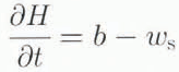
where w_s is the downward velocity at the surface and b is the snow-accumulation rate. Measurements of b during the interval 1989–92 give (1.17 ± 0.05)m a⁻¹. Deduction of w_s, from stratigraphic age vs depth gives (1.17 ± 0.01)m a⁻¹. Thus, within ±0.06 m a⁻¹, H did not change from 1989 to 1992. The equality between w_s and b over the interval 1989–92 must be viewed as accidental. Although w_s is slowly varying, there is high frequency variability in b(t) (shown below). It is more useful to compare w_s to a longer-term average of b afforded by the depth distribution of layer thickness. After considering the accumulation history, we return to the question of long-term thickness change.

7.2. Vertical pattern of mass change

The variation of density with depth describes the vertical distribution of mass (Fig. 8). In steady state, thickness H, density ρ(h) and downward velocity w(h) are independent of time. We now examine whether the profiles of w(h) (Fig. 5) and ρ(h) (Fig. 8) as observed in 1990–92 are consistent with steady state, by investigating conservation of mass at different depths in the firn.

Conservation of mass requires that

(5)

where ė_d(h,t) is the horizontal velocity divergence. (In Equation (5), D/Dt represents the time derivative following a parcel of matter, i.e. the material time derivative.) Based on Equation (5), the total rate of vertical compression

(6)

can be partitioned into a compactive part

(7)

and a dynamic part ė_d(h, t) such that

(8)

If it is assumed that horizontal gradients in ρ are negligible, the material time derivative of ρ may be evaluated as

(9)

Then conservation of mass Equation (5)) reduces to

(10)

Equation (10) shows that the local rate of density change results from the sum of the vertical and horizontal mass-flux divergences.

Below a depth of about 100 m, where ρ is close to ice density, both ∂ρ/∂t and ∂ρ/∂h are 0. Consequently, ė_d = −∂w/∂h, which is determined by the vertical strain measurements (Fig. 6). Just beneath 100 m, −∂w/∂h = (1.8 ± 0.1) × 10⁻³ a⁻¹. That rate is nearly identical to the horizontal velocity divergence measured at the surface, ė_d = (1.9 ± 0.1) × 10⁻³ a⁻¹. Thus, it is reasonable to assume that over the depth range of the firn layer ė_d is independent of depth and equal to the value at the surface.

With ė_d specified in the firn layer, it is possible to use Equation (10) to test whether ρ(h, t) is independent of time. Calculations were made using the smoothed representations of w and ρ shown in Figure 5 and 8. The horizontal and vertical mass-flux divergences do not balance, with the consequence that ρ(h, t) is predicted to be increasing in the upper part and decreasing in the lower part of the firn layer (Fig. 9). Changing the value of w_s assumed in the calculation shifts the curve for ∂ρ/∂t up and down in Figure 9, but does not significantly alter the shape of the depth dependence.

Fig. 8.

Density vs depth. Points show results from measurements on the ice core (Reference Thompson,Thompson and others, 1994). Solid curve shows a function fit to data. Dashed curve shows density required for steady mass distribution with measured vertical velocity and horizontal velocity divergence.

Fig. 9.

Rate of density change predicted from the balance of horizontal and vertical mass-flux divergence (Equation (10)) calculated with ė_d = 1.9 × 10⁻³ a⁻¹ and w_s = 1.17 m a⁻¹.

The inconsistency between ρ(h), w(h) and ė_d for steady state is further illustrated by solving Equation (10) with ∂ρ/∂t = 0 for (i) w(h) assuming the measured ρ(h) and ė_d (dashed curve in Figure 5), (ii) ρ(h) assuming the measured w(h) and ė_d (dashed curve in Figure 8), and (iii) ė_d assuming the measured w(h) and ρ(h) (dashed curve in Figure 6). The distributions predicted for w(h) and ρ(h) predicted by (i) and (ii) are well outside the range of measurement error. The distribution of ė_d(h) predicted by (iii) is unrealistically complex.

In combination these considerations show that the mass distribution is not steady.

7.3. Mass balance of the column

Denote the rate of change of mass in the column over the fixed range of depth from h₁ to h₂ by is determined by integration of Equation (10) over [h₁, h₂]. When dH/dt = 0 and h is in the ice beneath the firn, gives the mass balance of the full ice column. (This is true in this case, since the mass does not change above 0 or below h.) A value of h = 120 m somewhat below the firn-ice transition is convenient.

Figure 10 shows how depends on the choice of w_s and ė_d. Preferred values are w_s = (1.17 ± 0.01) m a⁻¹ and ė_s = (1.9 ± 0.1) × 10⁻³ a⁻¹, which imply a rate of mass change of (17 ± 10) kg m⁻² a⁻¹ (water equivalent thickness 0.017 m a⁻¹, ice-equivalent thickness 0.019 m a⁻¹) or about 4% of the annual accumulation (0.54 m a⁻¹ ice equivalent). A zero rate of mass change would be achieved with the measured ė_d, if w_s were 1.21 m a⁻¹. (The increment of 0.04 m a⁻¹ downward motion results in a larger increase in mass flux lost through the firn-ice transition than gained at the upper surface, which follows from the differences in density at these locations.) Such a high value of w_s appears to be inconsistent with the stratigraphically determined age vs depth as discussed above. A zero rate of mass balance could also be achieved by increasing horizontal velocity divergence to 0.0021 a⁻¹, which is slightly larger than expected from measurements. Alternatively, a surface density of 15 kg m⁻³ lower than implied by measurements (Fig. 8) would predict zero balance, which is in the range of measurement error. Therefore, it appears that the mass is increasing at present, but the rate is not distinctly above measurement error.

Fig. 10.

Inferred column mass balance depending on downward velocity at surface w_s and horizontal flow divergence ė_d. Lines show contours of equal mass balance in units of kg m⁻² a⁻¹. Box shows expected ranges for w_s and ė_d.

8. Accumulation-rate History

The thicknesses of annual firn layers l(h, t) measured in a core contain information about the history of snow accumulation b[t − A(h, t)]. It is necessary to account for thinning of layers Since their times of deposition. The rate of thinning of a layer is given by

(11)

The total compressive (logarithmic) strain over the time interval from deposition t₀ = t − A(h, t)[t₀, t] to measurement t is found by integration of Equation (11) over [t₀, t] to be

(12)

Integration of Equation (6) gives an alternative evaluation of e(h, t) from the vertical velocity w. We assume that H and w are independent of time over the time interval [t₀, t] as the layer moves over the depth range [0, h]. Then integration of Equation (6) over [t₀, t] using ∂w/∂h = w⁻¹ dw/dt gives

(13)

Comparison of Equations (12) and (13) implies that

(14)

which determines initial snow thickness l(0, t₀) from the in situ firn layer thickness l(h, t) and velocity w(h, t). If the density profile is assumed to have been constant, then the corresponding initial mass per unit area (m(0, t₀) = ρ(0, t)l(0, t₀)) and in situ (m(h, t) = ρ(h, t) l(h, t)) are related by

(15)

This gives the water-equivalent thickness. It can be converted to ice-equivalent thickness using ice density.

Results derived from Equations (14) and (15) using l(h, 1990) (in situ firn), the smoothed velocity profile (Fig. 5) with w_s, = 1.17 m a⁻¹ and the smoothed density profile (Fig. 8) are shown in Figure 11. Accumulation rate is shown as snow- (initial snow) and ice- (initial ice) equivalent thicknesses. The progressive thinning with depth of the in situ ice-equivalent thickness compared to the initial ice-equivalent thickness represents export of ice from the column by dynamic strain associated with horizontal velocity divergence (spreading). The thinning of in situ firn thickness in comparison to in situ ice-equivalent thickness represents vertical compaction by densification. The curves in Figure 11 are smoothed with 20 year running means. The mean ice-equivalent accumulation rate for the record length is 0.53 m a⁻¹.

Fig. 11.

History of annual snow accumulation (initial snow) and corresponding ice-equivalent thickness (initial ice equivalent). The physical thickness (in situ firn) and ice-equivalent thickness (in situ ice equivalent) of annual layers in the 1990 core vs time of deposition are shown for comparison.

Figure 12 shows the ice-equivalent accumulation rate vs time at an expanded scale, and includes unsmoothed results. There are prominent decadal variations in most of the record, two multi-decade peaks of high accumulation rate around AD 1550 and 1600, a trend of decreasing accumulation rate from the early to late 18th century and a gradual increase from the late 18th century to the present. The record shows strong interannual variations; however, many of these annual-scale variations are artifacts that arise by assignment of annual boundaries from stratigraphic features that do not occur at consistent calendar dates.

Fig. 12.

Ice-equivalent annual accumulation. Smooth heavy curve shows 20 year running mean. Light curve shows unsmoothed results.

9. Discussion

9.1. Ice dynamics at the summit

The geometry and flow pattern are complex (Figs 2 and 3), because of the mountainous sub-ice terrain. The motivation to core at a summit is especially strong in these circumstances, since ice displaced over the rugged bed relief is likely to have experienced complex deformation. The location of the ice summit near the 1990 core site is probably associated with the high sub-ice terrain beneath it, and its position may be quite stable. The relatively small ice thickness allows access to ice of a given age at a smaller depth than at surrounding locations with larger thickness. Thus, the site could be considered for deeper coring in the future. In this regard the depth variations of vertical velocity and strain are relevant beneath the lowest measurements.

If w_s (1990) = 1.17 m a⁻¹ is assumed as discussed above, then the velocity of the lowest marker (Fig. 5) is given by Equation (1) as w(201, 1990) = 0.19 m a⁻¹. The Frozen condition of the bed (h = 365 m) requires that w(365, 1990) = 0. This condition enables extension of the velocity profile to the bed. A smoothing function matching the measurements of differential velocity (Fig. 5), w_s = 1.17 m a⁻¹ and w(365, t)= 0 yields an essentially linear variation of w over the interval [201, 365].

The age vs depth that results from Equation (3) with this distribution of w over the full depth (Fig. 13) predicts ages of about 2500 a at 20 m above the bottom. The corresponding factors for correction of layer thickness and mass per unit area given by Equations (14) and (15) are about 40 and 20 respectively at that depth (Fig. 14). The actual depth to which these predictions of age and strain effects remain reliable is uncertain, because of the potential for disturbance of stratigraphy near the bed. Furthermore, as discussed below, a linear variation of w must break down very close to the bottom. It is unlikely that a reliable record longer than a few thousand years could be obtained at this location, because the older ice is very thin. The limitation on the age arises because of the low ice thickness at this location and generally high accumulation rate.

Fig. 13.

Dynamic age extended to near the base of the ice.

Fig. 14.

Corrections for layer thickness and mass per unit area extended to near the base of the ice.

The velocity difference between 201 m and the bed determines the mean rate of vertical compression −∂w/∂h = 0.0012 a⁻¹ over the depth interval [201, 365]. Comparison with ė_d over [0, 201] indicates that ė_d is relatively independent of depth below 200 m (Fig. 15). The frozen-bed condition imposes −∂w/∂h = 0 at the bed, but the zone of small −∂w/∂h must be confined very close to the bed in order to fit the requirements imposed by the average over the interval [201, 365].

Fig. 15.

Vertical strain rate inferred for the full depth. Short dashes show average strain rate below deepest measurements assuming w_s = 1.17 m a⁻¹. Long dashes show ė_d measured at surface and assumed for the thickness of the firn layer.

The nearly depth-independent strain rate conflicts with theoretical models of the flow at a divide with low bed relief, which predict strong gradients in −∂w/∂h in the central part of the ice thickness with a thick zone of lower than average strain rate above the bed (Reference Raymond,Raymond, 1983; Reference Reeh,Reeh, 1988). This difference probably arises because of the sharp sub-ice ridge (Fig. 3). Because the bed falls away steeply on either side, horizontal Spreading is not constrained by the frozen bed as strongly as it would be if the bed were flat. In comparison to a flat bed, there are related consequences: downward motion remains relatively high close to the bed; the ice is not as old at a given depth; the oldest ice is not as thick. Thus, some of the age-vs-depth advantage associated with a flow divide is lost over a sharp peak. This behavior needs to be borne in mind more generally when considering coring sites over sub-ice peaks, where standard models of age vs depth may fail.

The age-vs-depth relationship at the 1990 core site can be extended to other locations in its vicinity by tracing internal radar reflectors, assuming these are isochronous stratigraphic horizons. Reference Weertman,Weertman (1993; paper in preparation) discusses this means of establishing the three-dimensional age-field of the ice. Thicker sequences of ice much older than several thousand years can be accessed at deeper locations nearby, but at greater depth.

10. Summary

The core site on the crest of the Dyer Plateau is positioned over a subglacial ridge, which should serve to anchor the position of the ice summit. The ice sheet in the vicinity of this summit is currently close to steady state. The present rate of thickness change is less than 10% of the annual rate of snow accumulation of about 1.17 m a⁻¹. Some degree of non-steady state is indicated by the vertical variations of density and downward velocity, which imply a non-steady density profile in the firn. The mass in the uppermost 100 m is increasing at a rate of approximately 4% of the mass-accumulation rate.

Deviations from perfect steady state are expected, because the accumulation rate defined by the thickness of annual layers has increased progressively from 0.46 to 0.54 m a⁻¹ ice equivalent over the interval from about AD 1790 to the present. There were prominent multi-decadal variations in accumulation rate during the 16th century. There is no evidence for a long time-scale trend in accumulation rate over the 500 a period covered by the core. However, the possibility of such a trend cannot be eliminated.

The combination of high accumulation rate, small local thickness and associated ice-flow pattern near the summit limits the length of record that can be achieved with confidence at that location to a few thousand years. Older records are possible at nearby locations on the Dyer Plateau flow divide where the thickness is larger.