1 Introduction
Vortex breakdown is a characteristic phenomenon affecting swirling jet and wake flows. It is associated with a sudden change of the flow topology when the swirl number
 $S$
, defined as the ratio between the characteristic tangential velocity and the centreline axial velocity, reaches a critical value. While the flow remains columnar below this threshold, it suddenly changes topology into several possible vortex breakdown states, which have been observed and labelled across the last decades. As first observed by Lambourne & Bryer (Reference Lambourne and Bryer1962) on delta-wings, both the bubble vortex breakdown characterized by an axisymmetric recirculation region and the spiral vortex breakdown can exist in similar flow conditions. Even richer dynamics and structures have been observed in tube experiments by Hall (Reference Hall1972), Leibovich (Reference Leibovich1978) and Escudier & Zehnder (Reference Escudier and Zehnder1982) where the bubble breakdown may be followed by columnar, single spiral or double spiral flows, depending on the parameters. In this vein, Sarpkaya (Reference Sarpkaya1971) reported a flow map of the different possible states with respect to the bifurcation parameters. Vortex flows possibly experiencing vortex breakdown are found in several industrial applications, such as flow over delta-wings, thermal and hydraulic turbomachines as well as combustion chambers. In these industrial situations, vortex breakdown often results in performance degradation and structure fatigue although in certain case it may be also beneficial, for example in burner stabilization where the stagnation point plays the role of flame anchor. High performance industrial exploitation of these systems under secure operating conditions therefore calls for flow control techniques which could enable operating in the off design regime and thereby increase operating flexibility (European policy 2017), see among others Susan-Resiga et al. (Reference Susan-Resiga, Muntean, Hasmatuchi, Anton and Avellan2010), Favrel et al. (Reference Favrel, Müller, Landry, Yamamoto and Avellan2015), Pasche, Avellan & Gallaire (Reference Pasche, Avellan and Gallaire2017) for hydraulic turbomachines and Gursul, Wang & Vardaki (Reference Gursul, Wang and Vardaki2007) for leading-edge vortices and Paschereit, Flohr & Gutmark (Reference Paschereit, Flohr and Gutmark2002), Syred (Reference Syred2006) for thermal turbomachines.
To interpret the variety of observed vortex breakdown states, two different physical mechanisms were mainly highlighted over the years. First, the transition from columnar flow to bubble breakdown was interpreted by Squire (Reference Squire1960) as the consequence of an infinitesimal standing wave, which exists only when the swirl surpasses a certain threshold. In addition, Benjamin (Reference Benjamin1962) showed that this threshold coincides with the super/subcritical transition where Kelvin waves hosted by the vortex core start propagating upstream. This led him to draw an analogy with the hydraulic jump phenomenon, known to be also associated with a super/subcritical transition of gravity waves. Since then, Wang & Rusak (Reference Wang and Rusak1997) have proposed a unifying view connecting these local wave propagation properties to the global stability properties of inviscid vortex flows of finite length.
Second, the hydrodynamic instabilities of swirling jets and wakes have been analysed in great detail with emphasis on the development in space and time of helical disturbances. While several mechanisms can be active for velocity profiles with strong axial or azimuthal shear (Gallaire & Chomaz Reference Gallaire and Chomaz2003), even vortex flows with Gaussian axial vorticity and velocity distributions, referred to as the Bachelor vortex, were found very unstable at intermediate values of swirl, as the result of the so-called generalized centrifugal instability (Leibovich & Stewartson Reference Leibovich and Stewartson1983). The observation that helical instability could become absolutely unstable (Huerre & Monkewitz Reference Huerre and Monkewitz1990) in swirling wakes (Delbende, Chomaz & Huerre Reference Delbende, Chomaz and Huerre1998) has led to the interpretation of spiral vortex breakdown as a secondary instability of axisymmetric vortex breakdown (Gallaire et al. Reference Gallaire, Ruith, Meiburg, Chomaz and Huerre2006). The absolutely or convectively unstable nature of the flow was determined by computing numerically the linear impulse response of a localized disturbance on the numerically computed axisymmetric flow solution, as previously performed by Ruith et al. (Reference Ruith, Chen, Meiburg and Maxworthy2003). The self-sustained instability accounting for spiral vortex breakdown was interpreted as the consequence of the existence of an absolutely unstable region.
Ruith et al.’s (Reference Ruith, Chen, Meiburg and Maxworthy2003) direct numerical simulations (DNS) of the incompressible Navier–Stokes equations were probably the first attempt to break the dependence on the lateral boundary condition in comparison with previous studies such as Spall, Gatski & Ash (Reference Spall, Gatski and Ash1990), Althaus et al. (Reference Althaus, Krause, Hofhaus and Weimer1994). In addition to axisymmetric direct numerical simulations, the author also performed full three-dimensional (3-D) DNS, using convective radial boundary condition mimicking a semi-infinite domain, in order to analyse the mode selection in a free-vortex breakdown phenomenon. The flow solutions were initiated by the inlet (Grabowski & Berger Reference Grabowski and Berger1976) vortex profile and this vortex now appears as a benchmark model for disturbance analysis of the vortex breakdown in the more recent work of Vyazmina et al. (Reference Vyazmina, Nichols, Chomaz and Schmid2009), Meliga, Gallaire & Chomaz (Reference Meliga, Gallaire and Chomaz2012a
), Qadri, Mistry & Juniper (Reference Qadri, Mistry and Juniper2013), Rusak, Granata & Wang (Reference Rusak, Granata and Wang2015). Both Meliga et al. (Reference Meliga, Gallaire and Chomaz2012a
) and Qadri et al. (Reference Qadri, Mistry and Juniper2013) performed a global linear stability analysis about the axisymmetric base flow, and successfully described the Hopf bifurcation and the development of the spiral vortex breakdown spinning in time around the axisymmetric breakdown bubble for Reynolds number and swirl number close to
 $Re=200$
and
 $S=1$
, confirming the weakly non-parallel local analysis of Gallaire et al. (Reference Gallaire, Ruith, Meiburg, Chomaz and Huerre2006). Furthermore Meliga et al. (Reference Meliga, Gallaire and Chomaz2012a
) used the global stability analysis to rigorously derive coupled weakly nonlinear amplitude equations that helped understanding the mode selection between a single spiral
 $m=1$
and a double spiral
 $m=2$
in the vicinity of the codimension-2 point
 $Re=71.95$
and
 $S=1.436$
.
Such global stability analyses about the axisymmetric base flow are relevant at the instability onset but one may question their validity further away from the threshold. This fundamental issue, related to the application of global stability analysis to real flows, was revived by Barkley (Reference Barkley2006). Considering the Bénard–von Kármán vortex street in the cylinder wake, Barkley (Reference Barkley2006) showed that the Strouhal number was correctly captured by a global linear stability analysis around the mean flow while the prediction from the linearization around the base flow quickly failed when the Reynolds number was increased. This can be interpreted as a consequence of the mean flow distortion (Maurel, Pagneux & Wesfreid Reference Maurel, Pagneux and Wesfreid1995) resulting from the nonlinear Reynolds stresses, which accounts for both the difference between the base and mean flow and for the saturation of the disturbance, as demonstrated by Sipp & Lebedev (Reference Sipp and Lebedev2007) using a weakly nonlinear multiple-scale expansion to derive a Landau amplitude equation. More recently, this approach was extended further away from the threshold (Mantič-Lugo, Arratia & Gallaire Reference Mantič-Lugo, Arratia and Gallaire2014) by a semilinear coupling of, on the one hand, the correction to the base flow through the Reynolds stresses, to, on the other hand, a linearized disturbance equation. Without going into that level of analysis, we will in the present study address the quality of the frequency prediction resulting both from the stability analysis about the base and mean flows in Ruith et al.’s (Reference Ruith, Chen, Meiburg and Maxworthy2003) semi-infinite swirling flow configuration by considering Reynolds numbers up to
 $Re=500$
.
Recently local and global stability analyses about mean and turbulent mean swirling flows experiencing vortex breakdown were investigated in several confined geometries. Among others, Tammisola & Juniper (Reference Tammisola and Juniper2016) investigated the flow in a swirl generator set-up at a Reynolds number of
 $4.8\times 10^{3}$
, Oberleithner et al. (Reference Oberleithner, Sthr, Im, Arndt and Steinberg2015) and Paredes et al. (Reference Paredes, Terhaar, Oberleithner, Theofilis and Passchereit2015) studied the precessing vortex core in a combustion chamber at a Reynolds number of approximately
 $3\times 10^{4}$
. Grimble, Agarwal & Juniper (Reference Grimble, Agarwal and Juniper2017) considered the flow in a cyclone separator set-up at a Reynolds number of approximately
 $10^{4}$
and Pasche et al. (Reference Pasche, Avellan and Gallaire2017) investigated the part load vortex rope in Francis turbines at a Reynolds number of approximately
 $10^{6}$
. These studies successfully predict the unstable nature of the helical mode and its frequency. This helical mode structures the flow and acts as an excitation source in these industrial applications. The growth rate resulting from the stability analysis moreover can define a measure to assess control efficiency or can be used as an input to investigate relevant control strategies such as feedback or predictive control. Control techniques applied to Navier–Stokes equations were reviewed by Kim & Bewley (Reference Kim and Bewley2007), and can be categorized for our purpose into two main approaches: the closed-loop and open-loop control strategies. Among open-loop control strategies, one distinguishes between passive and active strategies, the latter being subcategorized into steady and unsteady. All of these control approaches seek flow manipulations which aim at optimizing some features of the flow. The control target can be an eigenvalue, the drag on an obstacle, among many other possible choices of objectives.
Regarding first closed-loop control, foundations were laid by Lions (Reference Lions1971), who demonstrated the existence and the uniqueness of the optimal control solution for linear partial differential equations and quadratic objectives. Such predictive techniques were initiated by Joslin et al. (Reference Joslin, Gunzburger, Nicolaides, Erlebacher and Hussaini1997) and Bewley, Moin & Temam (Reference Bewley, Moin and Temam2001). They are computationally extremely demanding, because of the need to perform unsteady direct and adjoint calculations, with the associated memory requirements. With the recent advent of high performance computing facilities (HPC), there is a certain revival in the approach (Passaggia & Ehrenstein Reference Passaggia and Ehrenstein2013; Goit & Meyers Reference Goit and Meyers2015). An alternative closed-loop control approach, inspired by automatic control and based on direct feedback control, was promoted in the hydrodynamic instability context by Bewley & Liu (Reference Bewley and Liu1998), among others. The closed-loop control couples actuators to sensors for optimal disturbance rejection using a feedback gain matrix that is determined by solving a matrix Riccati equation. While several examples of direct feedback control can be found in the literature (see Kim & Bewley (Reference Kim and Bewley2007) for a review), they most often need to be combined with a model reduction technique.
Focusing next on steady open-loop control, although it can be based on trial and error (Strykowski & Sreenivasan Reference Strykowski and Sreenivasan1990), it can also be determined within an adjoint-based optimization approach. This approach is derived in the Lagrangian functional framework and uses the adjoint fields as Lagrangian multipliers to determine a closed-form expression of the gradient direction in a very cost-effective way (Gunzburger Reference Gunzburger1999; Luchini & Bottaro Reference Luchini and Bottaro2014). The first gradient direction may be viewed as the sensitivity field, following Giannetti & Luchini (Reference Giannetti and Luchini2007) or Marquet, Sipp & Jacquin (Reference Marquet, Sipp and Jacquin2008). The sensitivity is defined as the gradient of the objective (for instance the eigenvalue) with respect to the control variable (for instance a distributed volume force). The sensitivity to base flow modification was applied to the stabilization of the cylinder wake flow by Marquet et al. (Reference Marquet, Sipp and Jacquin2008). More rarely does the adjoint-based optimization approach seem to have been used in its entire nonlinear spirit (Camarri & Iollo Reference Camarri and Iollo2010). The sensitivity analysis of the laminar and steady base flow solution was extended to the mean flow for turbulent flows by Meliga, Pujals & Serre (Reference Meliga, Pujals and Serre2012b ), focusing on nominally 2-D flow configurations, followed more recently by Mettot, Sipp & Bézard (Reference Mettot, Sipp and Bézard2014) and Carini et al. (Reference Carini, Airiau, Debien and Pralits2017).
Turning back to axisymmetric vortex breakdown, Gallaire, Chomaz & Huerre (Reference Gallaire, Chomaz and Huerre2004) applied Ricatti-based feedback control to quench the global axisymmetric unstable mode above the transition from supercritical to subcritical state for the inviscid flow in pipe of finite length, while Rusak et al. (Reference Rusak, Granata and Wang2015) recently implemented a more efficient physically based feedback control on the same flow. Steady open-loop wall control through blowing and suction was explored by Meliga & Gallaire (Reference Meliga and Gallaire2011) for viscous flow in a confined geometry and analysed in the framework of sensitivity analysis by determining the effect of the control on the amplitude equation governing the steady bifurcation. In the present study we will consider different steady open-loop flow control strategies to mitigate the development of the spiral mode in Ruith et al.’s (Reference Ruith, Chen, Meiburg and Maxworthy2003) flow. We will first attempt to minimize the radial velocity intensity as a proxy for the flow non-parallelism i.e. quenching the axisymmetric bubble, a strategy referred to as ‘optimal base flow manipulation’. Then we will devise an iterative scheme to optimally quench the dominant eigenvalue growth rate of the base and mean flows. This ‘optimal flow stabilization control’ determines what could be called a nonlinear sensitivity field to a steady force and determines the control amplitude, which becomes relevant to design efficient control appendages (Lacis et al. Reference Lacis, Brosse, Ingremeau, Mazzino, Lundell, Kellay and Bagheri2014).
The paper is organized as follows: the open geometry of Ruith et al. (Reference Ruith, Chen, Meiburg and Maxworthy2003) leading to spiral vortex breakdown is described together with the governing equations in § 2, while we perform unsteady 3-D DNS of the spiral vortex breakdown at various Reynolds numbers and determine the prevailing axisymmetric laminar base flow solution in § 3. This section is completed by a comparison of the stability properties of the base and mean flows, which are also compared to the limit cycle frequency obtained from the DNS. The theoretical framework for the optimal flow control problem is described in § 4 both for the optimal base flow manipulation and the base and mean flow stabilization approaches. The results of these different control strategies are compared in § 5, before conclusions are drawn.
2 Flow configuration
2.1 Governing equations
We consider the dimensionless incompressible Navier–Stokes equations in a semi-infinite domain
 $\unicode[STIX]{x1D6FA}$
,
 $$\begin{eqnarray}\left.\begin{array}{@{}c@{}}\displaystyle \frac{\unicode[STIX]{x2202}\boldsymbol{V}}{\unicode[STIX]{x2202}t}+(\boldsymbol{V}\boldsymbol{\cdot }\unicode[STIX]{x1D735})\boldsymbol{V}=-\unicode[STIX]{x1D735}P+Re^{-1}\unicode[STIX]{x1D6FB}^{2}\boldsymbol{V}\quad \text{in}~\unicode[STIX]{x1D6FA}\\ \unicode[STIX]{x1D735}\boldsymbol{\cdot }\boldsymbol{V}=0\quad \text{in}~\unicode[STIX]{x1D6FA},\end{array}\right\}\end{eqnarray}$$
where
 $(\boldsymbol{V},P)$
are the state variables and
 $Re$
the Reynolds number, built on the fluid’s kinematic viscosity and on the vortex core radius and incoming centreline streamwise velocity prevailing at inlet. This system is written in compact form as
 $$\begin{eqnarray}{\mathcal{N}}\unicode[STIX]{x2202}_{t}\boldsymbol{Q}+{\mathcal{M}}(\boldsymbol{Q})=\mathbf{0}\quad \text{in}~\unicode[STIX]{x1D6FA},\end{eqnarray}$$
where
 $\boldsymbol{Q}=(\boldsymbol{V},P)$
,
 ${\mathcal{M}}$
is the nonlinear evolution operator and
 ${\mathcal{N}}$
is the singular operator premultiplying the time derivative. We consider the dynamics governed by (2.1) and resulting from an inlet (Grabowski & Berger Reference Grabowski and Berger1976) vortex profile
 $$\begin{eqnarray}\left.\begin{array}{@{}c@{}}U_{R}(R)=0,\quad U_{\unicode[STIX]{x1D703}}(R)=S\unicode[STIX]{x1D6F9},\quad U_{Z}(R)=1,\quad \text{on}~\unicode[STIX]{x1D6E4}_{in}\\ \unicode[STIX]{x1D6F9}(R\leqslant 1)=R(2-R^{2}),\quad \unicode[STIX]{x1D6F9}(R>1)=1/R.\end{array}\right\}\end{eqnarray}$$
This vortex is composed of a unitary uniform dimensionless axial velocity component
 $U_{Z}=1$
, a null radial velocity component and a tangential velocity component with maximum intensity assigned by the swirl number
 $S$
and composed of a vortex core of dimensionless radius
 $1$
in solid body rotation and a potential decay outside the vortex core. In the present study, we fix the swirl number to
 $S=1.095$
but let vary the Reynolds number up to
 $Re=500$
, thereby restricting our investigation to the spiral vortex breakdown case, in contrast to pure bubble vortex breakdown or multiple helix vortex breakdown observed respectively at lower and larger swirl numbers (Ruith et al.
Reference Ruith, Chen, Meiburg and Maxworthy2003; Meliga et al.
Reference Meliga, Gallaire and Chomaz2012a
).
2.2 Direct numerical flow simulation
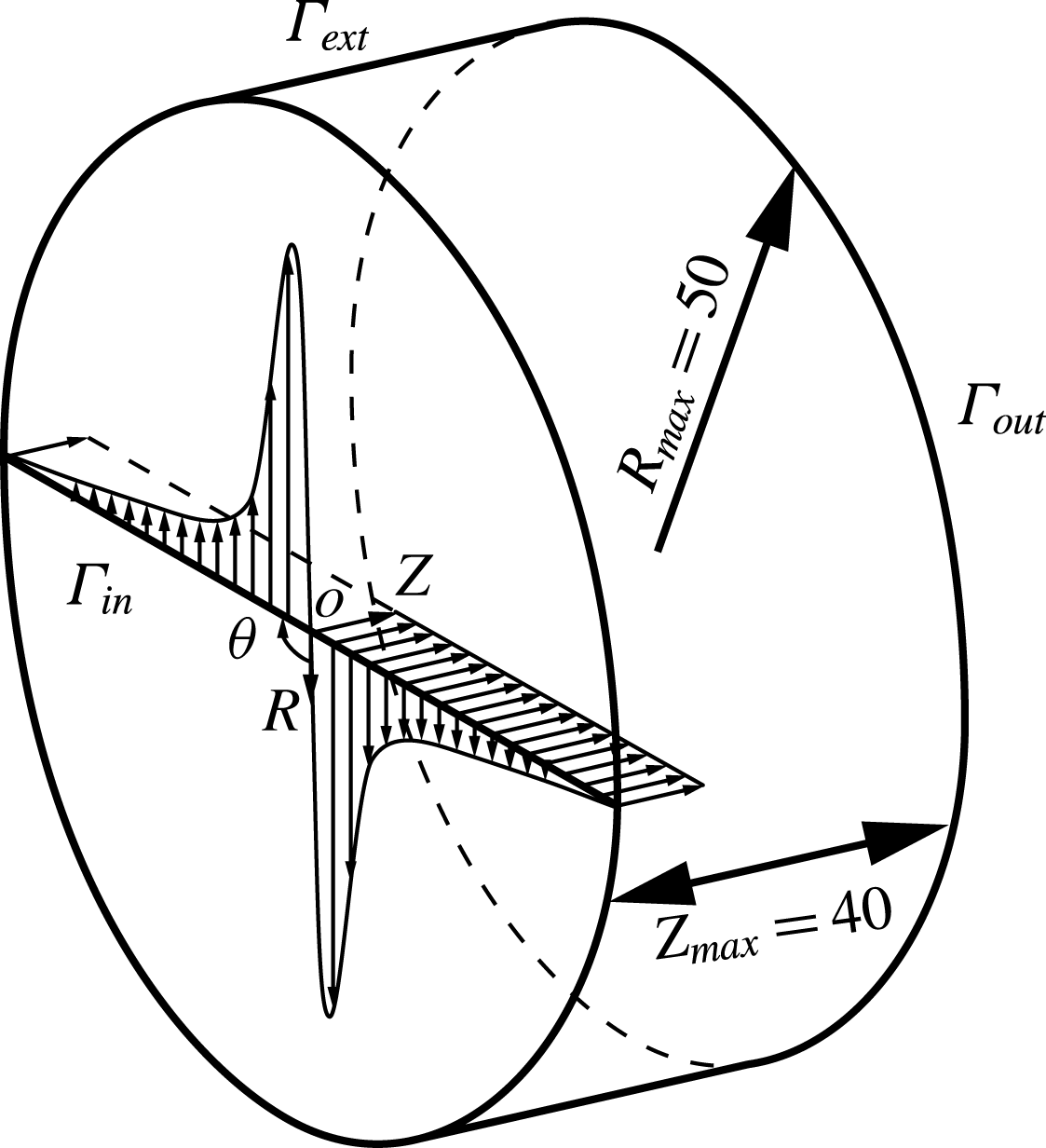
Direct numerical flow simulations have been performed on a 3-D cylindrical domain based on a Cartesian coordinate system
 $(X,Y,Z)$
. The main axis of the cylinder is oriented along the
 $Z$
-component and its origin is located at the centre of the inlet, see figure 1. A second, cylindrical, coordinate system is introduced
 $(R,\unicode[STIX]{x1D703},Z)$
, which is more convenient to study vortex flows, its axial axis
 $Z$
and origin remaining identical. The transformation matrix between the two reference frames is defined as follows: the
 $X$
-axis is oriented along
 $R$
for
 $\unicode[STIX]{x1D703}=0$
, while the
 $Y$
-axis completes the reference frame to obtain a right-handed coordinate system and corresponds therefore to
 $\unicode[STIX]{x1D703}=\unicode[STIX]{x03C0}/2$
. The radial extension of the domain equals
 $R_{max}=50$
while its length is
 $Z_{max}=40$
. Such dimensions were necessary to guarantee an unconfined radial boundary condition (see § A.1) because the vortex breakdown resulting from these flow conditions is known to be very sensitive to confinement effects, as experimented by Ruith et al. (Reference Ruith, Chen, Meiburg and Maxworthy2003). The computational domain is bounded by the Grabowsky and Berger vortex (2.3) on the inlet boundary
 $\unicode[STIX]{x1D6E4}_{in}$
, a free-outflow condition
 $(-P\boldsymbol{I}+Re^{-1}\boldsymbol{\cdot }(\unicode[STIX]{x1D735}\boldsymbol{V}))\boldsymbol{\cdot }\boldsymbol{n}=0$
on the external boundary
 $\unicode[STIX]{x1D6E4}_{ext}$
and a convective condition
 $\unicode[STIX]{x2202}_{t}\boldsymbol{V}+\boldsymbol{U}_{c}\boldsymbol{\cdot }\unicode[STIX]{x2202}_{\boldsymbol{n}}\boldsymbol{V}=0$
on the outlet boundary
 $\unicode[STIX]{x1D6E4}_{out}$
. We have fixed the convective velocity to be equal to the free-stream velocity
 $\boldsymbol{U}_{c}=\boldsymbol{e}_{Z}$
. The governing equations are solved numerically with NEK5000 a spectral element solver developed by Fischer, Lottes & Kerkemeier (Reference Fischer, Lottes and Kerkemeier2008). The temporal discretization of the nonlinear terms is treated explicitly by a third-order backward-differentiation scheme (BDF3) combined with a third-order extrapolation scheme (EXT3). The linear terms are treated implicitly in time and a pressure–velocity decoupling method is used for the spatial discretization. The velocity and pressure space are represented by a tensor-product array of Gauss–Lobatto–Legendre (GLL) and Gauss–Legendre (GL) points of polynomial orders
 $N$
and
 $N-2$
. In the present study,
 $P_{10}-P_{8}$
polynomial orders for velocity-pressure and 11 040 hexahedral elements are required to compute the flow field. This represents a computation of 8 million of degree of freedoms. The validation of the 3-D DNS is presented in § A.1.
Three-dimensional schematic of the flow configuration.

2.3 Axisymmetric flow
The steady axisymmetric flow solution developing from the inlet Grabowsky and Berger vortex (2.3) is also investigated, with governing equations written in compact form as
 $$\begin{eqnarray}\tilde{{\mathcal{M}}}(\boldsymbol{Q}_{B})=\mathbf{0}\quad \text{in}~\unicode[STIX]{x1D6FA}_{a},\end{eqnarray}$$
with
 $\boldsymbol{Q}_{B}=(\boldsymbol{V}_{B},P_{B})$
the base flow state variables. An axisymmetric domain
 $\unicode[STIX]{x1D6FA}_{a}$
, with the same dimensions as those of the 3-D domain is used
 $R_{max}=50$
and
 $Z_{max}=40$
, except that a sponge region is added along the
 $Z$
-component at the end of the domain. The length of this sponge region is equal to
 $L_{sponge}=60$
, using the same smoothing function as in Meliga et al. (Reference Meliga, Gallaire and Chomaz2012a
). The inlet and external boundary conditions are equivalent to those of the 3-D case but a symmetry condition is applied on the axis
 $\unicode[STIX]{x1D6E4}_{axis}$
that equals to
 $V_{BR}=V_{B\unicode[STIX]{x1D703}}=0,\unicode[STIX]{x2202}_{R}V_{BZ}=0$
, while the outlet boundary has a free-outflow condition.
The flow solution is carried out by the means of the finite element library Freefem++ (Hecht Reference Hecht2012). The steady axisymmetric incompressible Navier–Stokes equations are first premultiplied by
 $R$
to avoid the axis singularity and then solved numerically via a Newton–Raphson iterative method. The related linear system is carried out by the unsymmetric multifrontal sparse LU factorization package (UMFPACK). The computational domain is meshed by 408 866 triangular Taylor–Hood elements,
 $P_{2}-P_{1}$
polynomial-order elements for the velocity–pressure unknowns. A convergence criterion of
 $10^{-8}$
on the
 $H_{1}$
-norm is reached in the Newton–Raphson iterative method, which leads to the base flow solution.
2.4 Global stability analysis
The small disturbance dynamics,
 $\boldsymbol{q}^{\prime }=(\boldsymbol{v}^{\prime },p^{\prime })$
, of the Navier–Stokes equations is investigated by global linear stability analyses around the base flow
 $\boldsymbol{Q}_{B}$
and the mean flow
 $\bar{\boldsymbol{Q}}=(\bar{\boldsymbol{V}},\bar{P})$
in the axisymmetric domain
 $\unicode[STIX]{x1D6FA}_{a}$
. The disturbances
 $\boldsymbol{q}^{\prime }$
are expanded in normal modes for different azimuthal wavenumbers
 $m\in \mathbb{Z}$
,
 $$\begin{eqnarray}\boldsymbol{q}^{\prime }(R,\unicode[STIX]{x1D703},Z,t)=\boldsymbol{q}(R,Z)\exp (\text{i}(m\unicode[STIX]{x1D703}-\unicode[STIX]{x1D714}t))+\text{c.c.},\end{eqnarray}$$
where c.c. is the complex conjugate. We assume mean flow solutions unperturbed at first order by the Reynolds stresses (Barkley Reference Barkley2006, Meliga et al.
Reference Meliga, Pujals and Serre2012b
, Mantič-Lugo et al.
Reference Mantič-Lugo, Arratia and Gallaire2014 for discussion of this hypothesis). Therefore the eigenvalue problems related to the base and mean flow state become similar and may be written in a compact form using a generic flow solution
 $\boldsymbol{Q}_{0}=(\boldsymbol{V}_{0},P_{0})$
as
 $$\begin{eqnarray}[-\text{i}(\unicode[STIX]{x1D714}_{r}+\text{i}\unicode[STIX]{x1D714}_{i}){\mathcal{N}}+{\mathcal{L}}_{m}(\boldsymbol{V}_{0})]\boldsymbol{q}=\mathbf{0},\quad \text{in}~\unicode[STIX]{x1D6FA}_{a},\end{eqnarray}$$
where
 ${\mathcal{L}}_{m}$
is the operator for the linearized Navier–Stokes equations of azimuthal wavenumber
 $m$
and
 $\boldsymbol{Q}_{0}$
the linearization point that is equal to
 $\boldsymbol{Q}_{B}$
for the base flow eigenvalue problem and
 $\bar{\boldsymbol{Q}}$
for the mean flow eigenvalue problem. The time-averaged flow distribution
 $\bar{\boldsymbol{Q}}$
is computed on the fly in NEK5000 with a minimum of 160 periods of the characteristic oscillation, after the transient phase has died out. In addition, an interpolation step is needed to transfer the mean flow from the 3-D mesh to the axisymmetric mesh. This is carried out by a spectral interpolation of
 $10^{-13}$
accuracy integrated in NEK5000. At this level the mean flow is assumed purely axisymmetric and only a slice at
 $X=0$
and
 $Y>0$
is interpolated and exported to the eigenvalue solver.
In this context we use the definition that a positive azimuthal wavenumber
 $m>0$
corresponds to a spiral coiling in space in the anti-trigonometric direction and therefore, since
 $S>0$
, in the opposite direction as that of the ambient flow while
 $m<0$
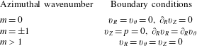
designates a spiral coiling in the same direction as the flow. The boundary conditions applied to the disturbances are homogeneous Dirichlet conditions when Dirichlet conditions are imposed on the base flow and remain unchanged in case of a Neumann condition. Specific boundary conditions, which are recalled in table 1, are applied on the symmetry axis due to the azimuthal expansion. They are obtained by symmetry considerations of the perturbations (Khorrami Reference Khorrami1991).
Boundary conditions on the axisymmetric axis applied to the disturbances for different azimuthal wavenumbers.

The global stability analysis is carried out by finite element method implemented in the Freefem++ software. The eigenvalue problem is first premultiplied by
 $R$
and then the discretized equations are solved by the implicit restarted Arnoldi method of the ARPACK library. The eigenvalues are obtained with a tolerance of
 $10^{-6}$
of the ARPACK solver. The axisymmetric mesh described in § 2.3 is used to compute the eigenvalue problem of the base and mean flow, except that the sponge region is removed for the latter. A validation of the eigenvalue calculations of the base and mean flows is presented in §§ A.2 and A.3 respectively.
3 Flow dynamics and stability analyses
3.1 Three dimensional flow
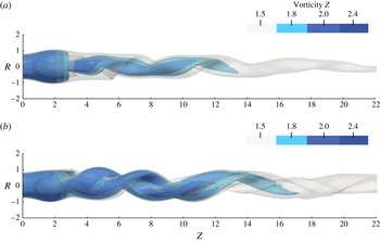
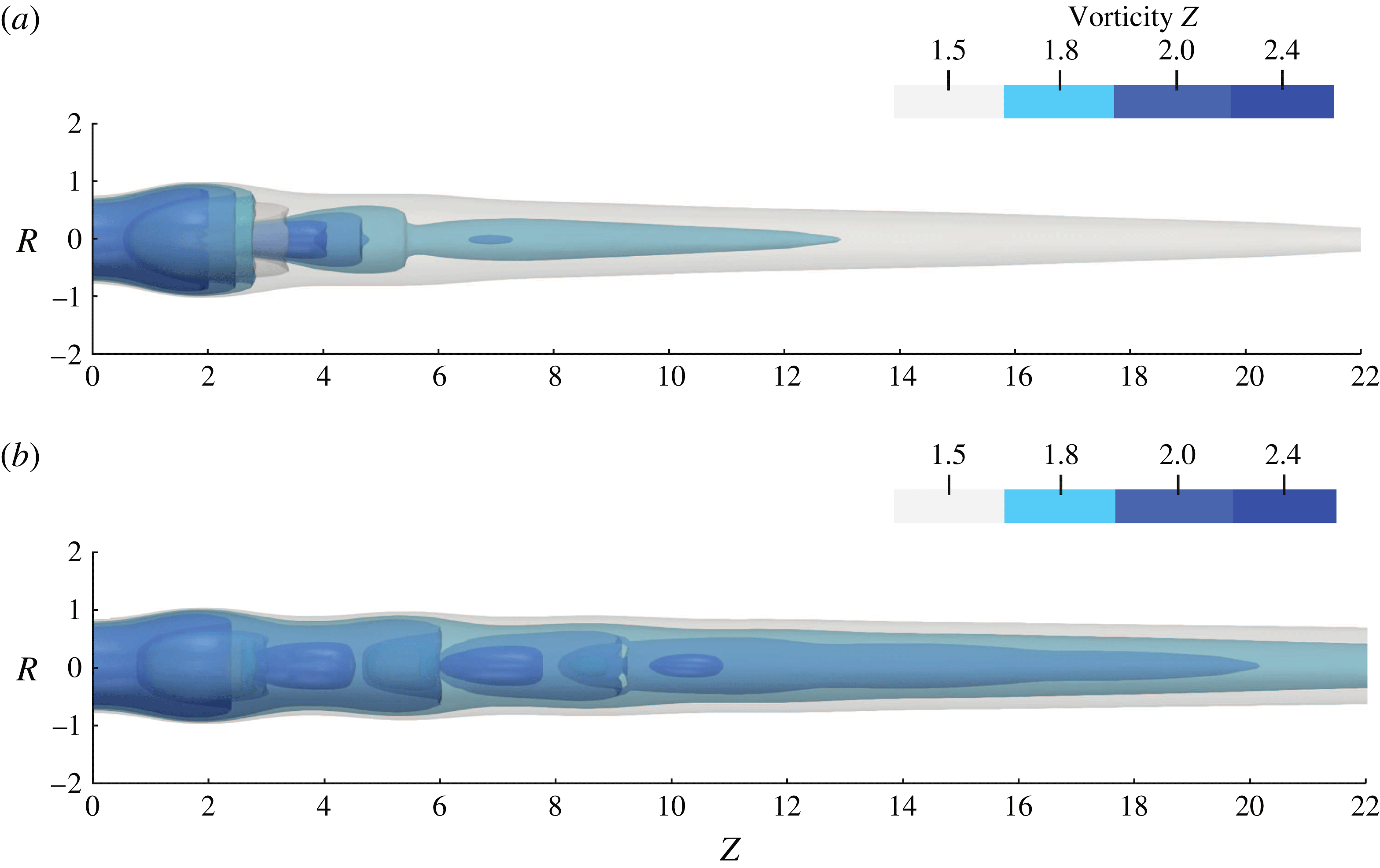
The 3-D instantaneous flow computations are illustrated for two specific Reynolds values,
 $Re=180$
and
 $Re=300$
, by axial vorticity contours in figures 2(a) and 2(b), respectively. These contours highlight the recirculation bubble and the spiralling motions of the flow. In the case of
 $Re=180$
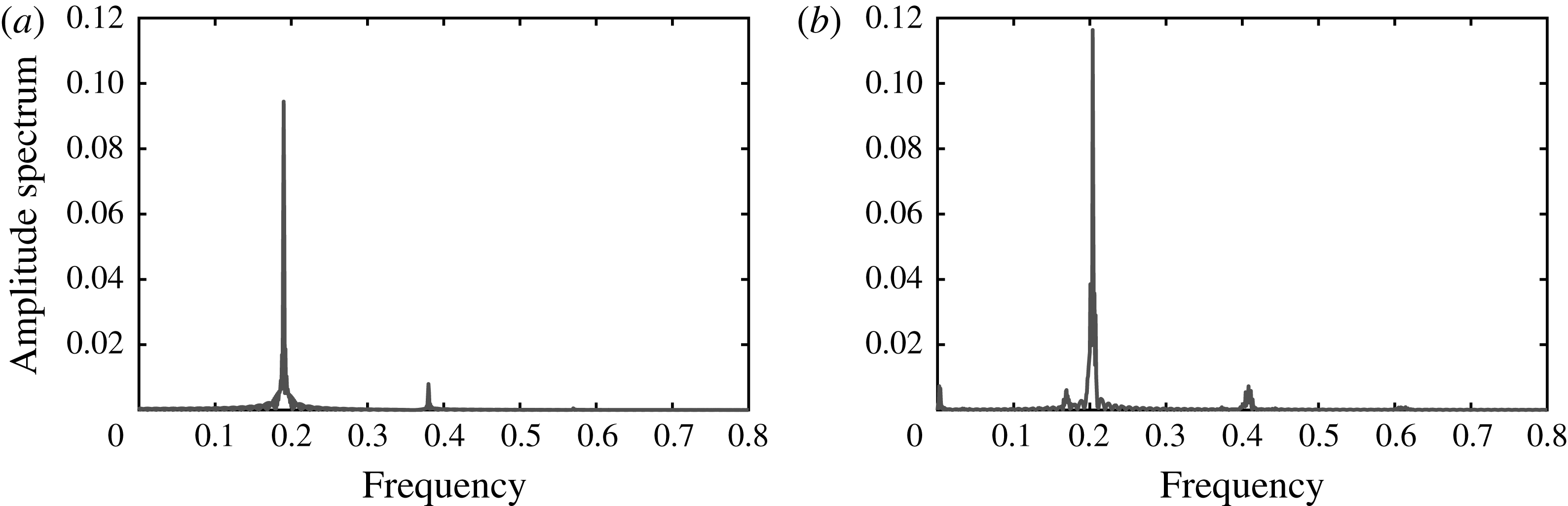
, the recirculation bubble is accompanied by a single helical vortex structure coiling in its wake, figure 2(a). The spiral spins temporally in the same direction as the Grabowsky and Berger vortex but coils spatially in the opposite direction, which is consistent with the previous results of Ruith et al. (Reference Ruith, Chen, Meiburg and Maxworthy2003). The temporal discrete Fourier amplitude spectrum of the radial velocity at the location
 $(R,\unicode[STIX]{x1D703},Z)=(0.1,0.0,5.0)$
, see figure 3(a), exhibits a quasi-sinusoidal signal at the frequency
 $f=0.189$
. The system has reached a limit cycle that arises from a self-sustained instability. In contrast, at
 $Re=300$
, the wake of the bubble is followed by two helical spirals, which have the same spatial coiling and temporal spinning as for
 $Re=180$
. The axial vorticity contours in figure 2(b) exhibit a second, slaved, spiral in the vicinity of first, master, spiral. They are differentiated by their axial vorticity magnitudes, the slaved structure exhibiting a modulated axial vorticity iso-contour when compared to the master structure, characterized by a dense iso-contour, at a value of 2.4. The temporal discrete Fourier amplitude spectrum is richer than that prevailing at
 $Re=180$
, see figure 3(b). This amplitude spectrum exhibits four peaks: a main one with a frequency of
 $f=0.204$
corresponding to the master helical vortex, a smaller peak close to the main peak with a frequency of
 $f=0.167$
, a low frequency peak at a frequency of
 $f=0.003$
as well as the main peak’s second harmonic at
 $f=0.408$
. The low frequency component and the broad base of the main peak, which latter is not due to a lack of fast Fourier transform (FFT) accuracy, are markers of the nonlinear interactions between the two spirals.
Iso-surfaces of axial vorticity contour of the 3-D DNS flow solution for (a)
 $Re=180$
and (b)
 $Re=300$
, for
 $S=1.095$
.

Discrete Fourier amplitude spectrum of the time signal of the 3-D DNS of the radial velocity component located at
 $(R,\unicode[STIX]{x1D703},Z)=(0.1,0.0,5.0)$
for
 $Re=180$
and
 $Re=300$
, for
 $S=1.095$
.

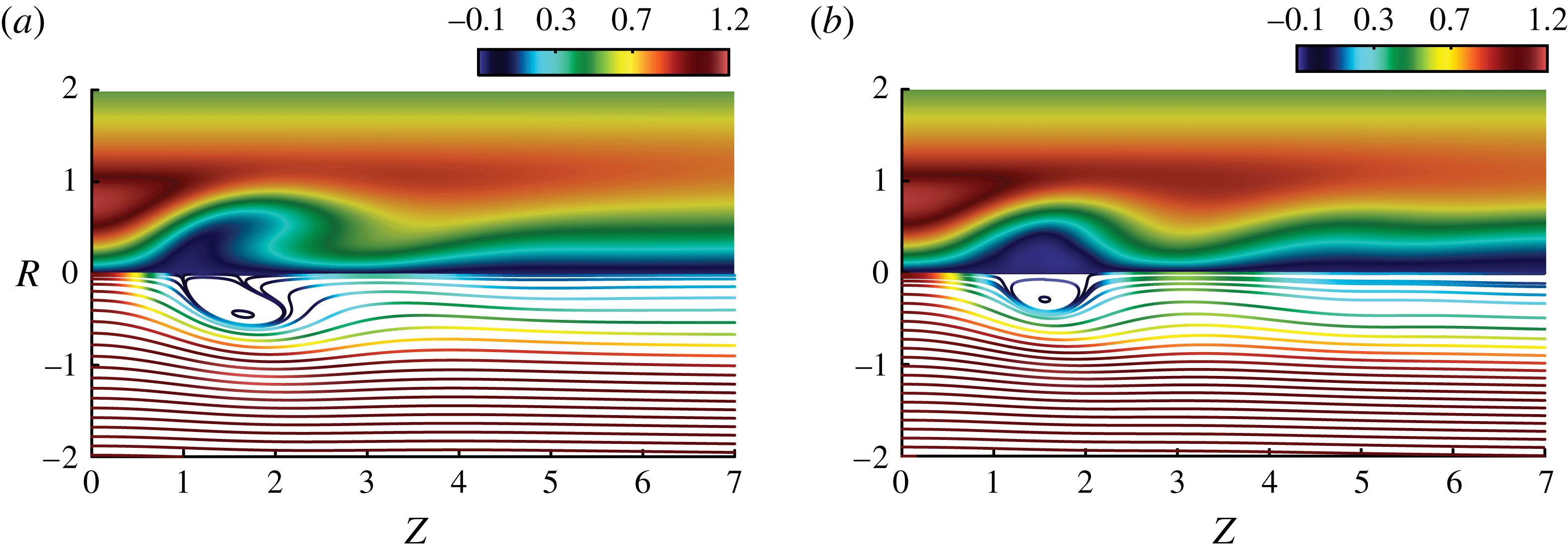
The axisymmetric time-averaged flow fields, to be investigated by global stability analysis, are displayed in figure 4. These figures are composed by the tangential velocity component on the upper part,
 $R>0$
, and streamsurfaces coloured by the magnitude of the axial velocity component on the lower part,
 $R<0$
. The time-averaged streamsurfaces exhibit a recirculation bubble, characteristic of vortex breakdown. At
 $Re=180$
, the bubble is elongated and lifted up from the centreline in its downstream part while the bubble has a more round shape for
 $Re=300$
, and additionally a second decelerated region is observed at
 $Z=5$
. We have observed that the extension of the time-averaged bubble decreases with the Reynolds number while the intensity of the undulating wake in the lee of the bubble increases with the Reynolds number.
3.2 Axisymmetric flow
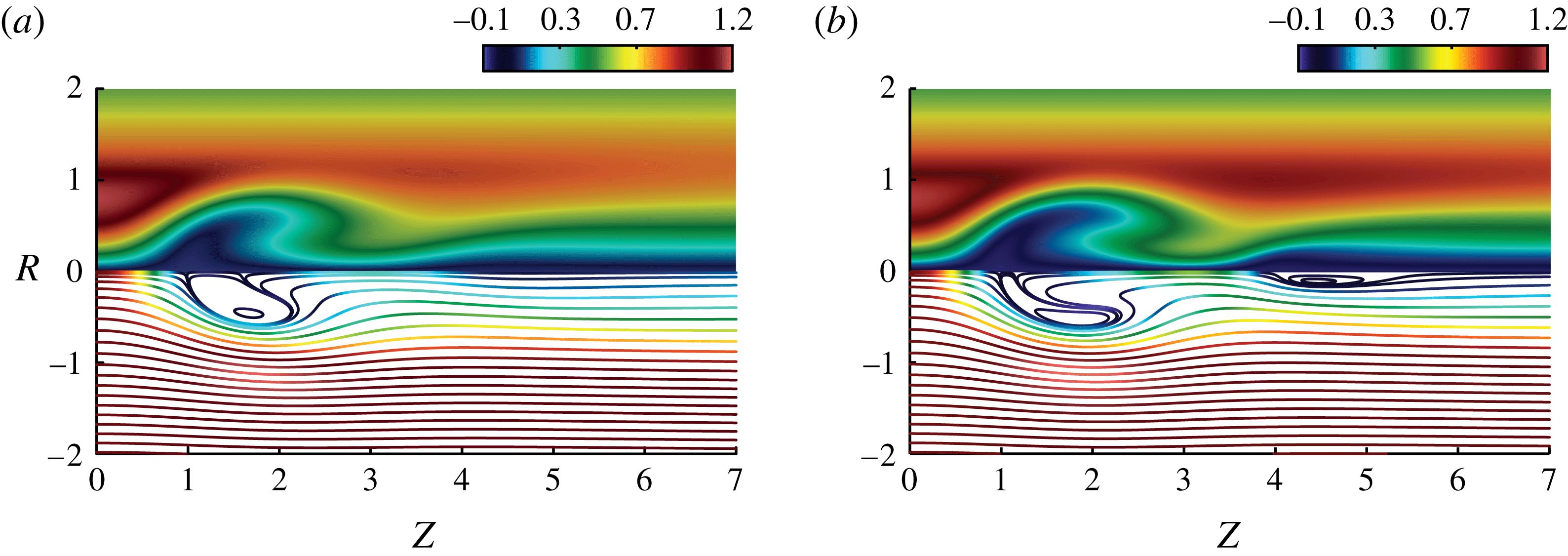
The axisymmetric base flow, governed by (2.4), is displayed in figures 5(a) and 5(b) for
 $Re=180$
and
 $Re=300$
, respectively, for
 $S=1.095$
. At a Reynolds value of
 $Re=180$
, the difference between the mean flow (figure 4
a) and the base flow (figure 5
a) is almost invisible. The mean flow correction resulting from the saturation of the self-sustained instability is therefore best observed at
 $Re=300$
, see figures 5(b) and 4(b), where the mean flow strongly deviates from the base flow, supporting the observations already reported by Ruith et al. (Reference Ruith, Chen, Meiburg and Maxworthy2003).
Time-averaged solution of the 3-D Navier–Stokes equations,
 $\bar{\boldsymbol{V}}$
, for
 $S=1.095$
and
 $Re=180$
(a) and
 $Re=300$
(b). The upper part of the graph shows the tangential velocity component and the lower part, the streamsurfaces coloured by the magnitude of the axial velocity component.

Solution of the steady axisymmetric Navier–Stokes equations,
 $\boldsymbol{V}_{B}$
, for
 $S=1.095$
and
 $Re=180$
(a) and
 $Re=300$
(b). The upper part of the graph shows the tangential velocity component and the lower part, the streamsurfaces coloured by the magnitude of the axial velocity component.

3.3 Global stability analysis
The global stability of the base flow and the mean flow have been investigated, with a focus on the first helical mode
 $m=1$
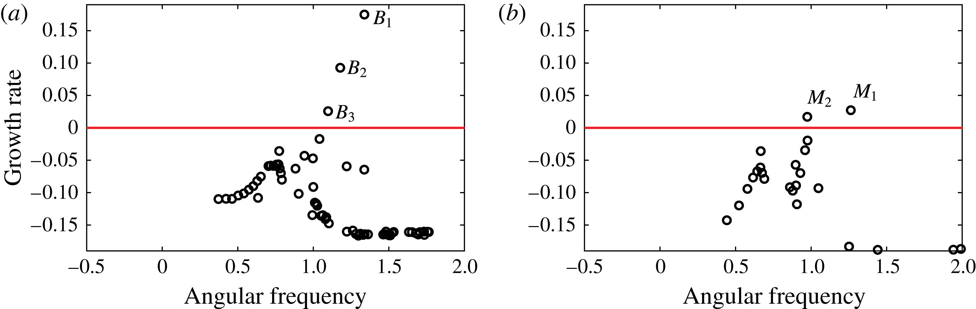
. A representative example is presented in figure 6 at a Reynolds value of
 $Re=300$
. Up to three unstable eigenmodes, labelled
 $B_{n}$
for
 $n=1,2,3$
can be identified in the eigenvalue spectrum of the base flow, while only two unstable modes
 $M_{1}$
and
 $M_{2}$
are detected in the mean flow eigenvalue spectrum. The associated growth rates are significantly larger when the linearization is performed around the base flow than around the mean flow, in agreement with mean flow modification based saturation mechanisms reported in different flow geometries (Barkley Reference Barkley2006; Mantič-Lugo et al.
Reference Mantič-Lugo, Arratia and Gallaire2014).
Eigenvalue spectra of the global linear stability of mode
 $m=1$
about the base (a) and mean (b) flow at
 $Re=300$
and
 $S=1.095$
. Unstable eigenvalues are labelled respectively
 $B_{1}$
,
 $B_{2}$
,
 $B_{3}$
and
 $M_{1}$
and
 $M_{2}$
.

We have then systematically compared the frequency prediction of the base and mean flow stability analyses for different Reynolds values
 $Re=100{-}500$
by keeping constant the swirl number
 $S=1.095$
, focusing only on unstable modes and on the azimuthal wavenumber
 $m=1$
, since other azimuthal wavenumbers were all found to be linearly damped. The instability threshold was found at
 $Re=143.5$
for the base flow and approximately at
 $Re=143.7$
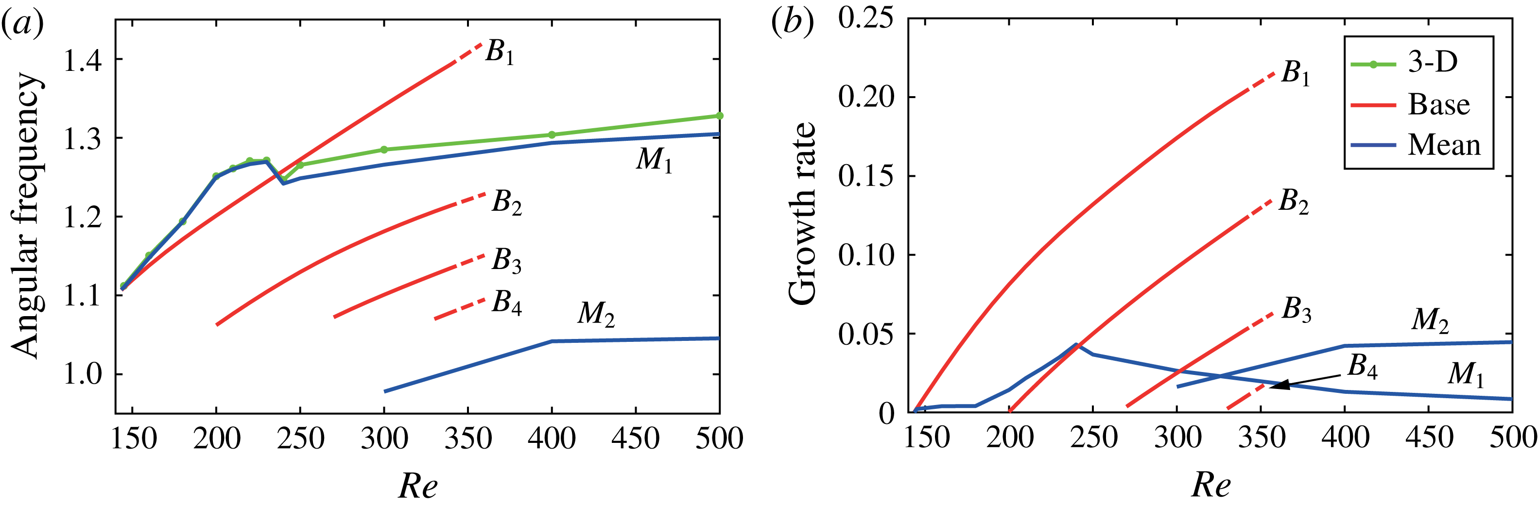
for the mean flow, where the dying out of the transient in the DNS become prohibitively long close to the threshold. In the vicinity of the threshold, the linear frequency predictions (respectively in red and blue for the base and mean flow) are in agreement with the limit cycle frequency extracted from discrete Fourier transform of the 3-D DNS signal (in green), see figure 7(a). As the Reynolds number increases, the growth rate of the dominant unstable mode linearized about the base flow (
 $B_{1}$
) increases rapidly, followed by a second unstable mode (
 $B_{2}$
) bifurcating at
 $Re=200$
and subsequently emerging unstable eigenvalues
 $B_{3}$
and
 $B_{4}$
. At
 $Re=350$
, where the base flow stability analysis has been stopped, the base flow is found to be unstable to no less than four unstable modes, as seen in figure 7(b). The frequencies of the four eigenvalues considered are all around
 $\unicode[STIX]{x1D714}_{r}\cong 1.08$
at their respective instability thresholds, beyond which they increase linearly with the Reynolds number. The base flow frequency prediction of the dominant unstable mode remains acceptable before it crosses the non-monotonic limit cycle frequency evolution (in green) around
 $Re=235$
. This appears as an a posteriori justification of the validity range of the linear stability analysis about the base flow of Meliga et al. (Reference Meliga, Gallaire and Chomaz2012a
) and Qadri et al. (Reference Qadri, Mistry and Juniper2013).
Growth rate and angular frequency of the global linear stability of the mean,
 $M_{1}$
,
 $M_{2}$
and base flow,
 $B_{1}$
,
 $B_{2}$
,
 $B_{3}$
,
 $B_{4}$
, for azimuthal wavenumber
 $m=1$
compared to the 3-D angular frequency from the DNS, computed by discrete Fourier transform at location
 $(R,\unicode[STIX]{x1D703},Z)=(0.1,0.0,5.0)$
.

The limit cycle frequency (in green) indeed first strongly increases away from the threshold until it drops for
 $Re>230$
and finally slowly increases with the Reynolds number for
 $Re>240$
. The frequency of the leading eigenvalue (
 $M_{1}$
) of the mean flow (in blue) closely follows the limit cycle frequency (in green) along the whole Reynolds number range, demonstrating a correct frequency prediction by the global stability analysis around the mean flow, as found in the canonical cylinder wake flow (Barkley Reference Barkley2006). Similarly the maximum growth rate of the mean flow remains much smaller that the growth rate of the dominant mode of the base flow that stays close to zero. Above
 $Re>300$
, a second unstable eigenvalue is found with a frequency that corresponds to the second peak observed in the temporal discrete Fourier amplitude spectrum (the angular frequencies
 $\unicode[STIX]{x1D714}_{r}$
should be divided by
 $2\unicode[STIX]{x03C0}$
to compare to the frequencies obtained in figure 3, for example at
 $Re=300$
,
 $f_{M_{2}}=0.156$
, and
 $f_{DNS}=0.167$
). The most unstable eigenmode is likely to correspond to the master helix. The second unstable eigenmode would be associated with the slaved helix. These frequency predictions, together with the global stability of the base and mean flows with respect to
 $m=2$
(not shown for brevity) are a confirmation that the snapshot of figure 2(b) at
 $Re=300$
does not correspond to an
 $m=2$
instability but rather to the superimposition of two
 $m=1$
spirals, each corresponding to a separate frequency peak and without any phase correlation.
These results on the frequency prediction of the stability analysis about the mean flow support the recent extension of this technique to high Reynolds number industrial flows, such as the frequency prediction of the precessing vortex core in a combustion chamber (Oberleithner et al. Reference Oberleithner, Sthr, Im, Arndt and Steinberg2015; Paredes et al. Reference Paredes, Terhaar, Oberleithner, Theofilis and Passchereit2015; Tammisola & Juniper Reference Tammisola and Juniper2016) or of the part load vortex rope in Francis hydraulic turbines (Pasche et al. Reference Pasche, Avellan and Gallaire2017). Moreover, we identify up to two unstable eigenmodes, which may offer a relevant test case for the need to take into account mode interaction in generalizing the self-consistent model for saturation dynamics developed by Mantič-Lugo et al. (Reference Mantič-Lugo, Arratia and Gallaire2014), in the spirit of the generalized quasi-linear models developed by Marston, Chini & Tobias (Reference Marston, Chini and Tobias2016).
4 Optimal control: flow stabilization and flow manipulation controls
4.1 Optimal control theory
Although it can be beneficial to improve mixing, the self-sustained instability in the spiral vortex breakdown is a source of perturbations that is undesirable in several applications (Rheingans Reference Rheingans1940; Syred Reference Syred2006; Gursul et al.
Reference Gursul, Wang and Vardaki2007; Nishi & Liu Reference Nishi and Liu2013). The finite amplitude nonlinear predictive control of such perturbations is investigated for two specific Reynolds values,
 $Re=180$
and
 $Re=300$
, with the aim of stabilizing the periodic fluctuations by applying a constant volume force. In the present study, we have chosen to minimize two different objectives to achieve this goal, a ‘flow stabilization control’ which targets a zero value of the growth rate of the most unstable eigenvalue declined into two versions controlling the base and mean flow eigenvalue, and a ‘flow manipulation control’ which targets a minimal radial velocity intensity. The rationale behind this latter choice is to minimize the radial flow associated with the bubble formation and thereby to maintain the flow as columnar as possible. This strategy is based on the physical mechanism underpinning spiral vortex breakdown: the wake induced by the bubble triggers an absolute instability region that leads to the spiral vortex oscillation (Gallaire et al.
Reference Gallaire, Ruith, Meiburg, Chomaz and Huerre2006; Qadri et al.
Reference Qadri, Mistry and Juniper2013). The mathematical framework required in these minimization problems is the optimal control theory. The objective functions for the two control strategies, to be defined in (4.1) and (4.2), are derived for the axisymmetric domain where the base flows and the relevant base and mean flow stability analyses were computed, bypassing larger and more expensive 3-D computations. This dimensionality reduction from the 3-D domain to a 2-D axisymmetric domain is performed thanks to the azimuthal Fourier decomposition naturally appearing in the eigenvalue analysis involved in the ‘flow stabilization control’. In the context of the ‘flow manipulation control’, only the axisymmetric base flow is considered, which is two-dimensional by definition. To be more specific the following objective functions are defined,
Flow manipulation control:
 $$\begin{eqnarray}\displaystyle \text{Min}\,{\mathcal{J}}_{Manip}(\boldsymbol{F})=\frac{1}{2}\int \!\!\!\int _{\unicode[STIX]{x1D6FA}_{a}}V_{R}(\boldsymbol{F})^{2}\,\text{d}\unicode[STIX]{x1D6FA}_{a}+\frac{\unicode[STIX]{x1D6FC}}{2}\int \!\!\!\int _{\unicode[STIX]{x1D6FA}_{a}}\Vert \boldsymbol{F}\Vert ^{2}\,\text{d}\unicode[STIX]{x1D6FA}_{a}, & & \displaystyle\end{eqnarray}$$
Flow stabilization control:
 $$\begin{eqnarray}\displaystyle \text{Min}\,{\mathcal{J}}_{Stab}(\boldsymbol{F})=|\text{Im}(\unicode[STIX]{x1D714})|+\frac{\unicode[STIX]{x1D6FC}}{2}\int \!\!\!\int _{\unicode[STIX]{x1D6FA}_{a}}\Vert \boldsymbol{F}\Vert ^{2}\,\text{d}\unicode[STIX]{x1D6FA}_{a}, & & \displaystyle\end{eqnarray}$$
where
 ${\mathcal{J}}$
is the objective function,
 $\boldsymbol{F}$
the control variable (here a volume force),
 $(\boldsymbol{V},P)$
are the state variables,
 $\unicode[STIX]{x1D714}$
is the eigenvalue of the most unstable eigenmode linearized around the base
 $\unicode[STIX]{x1D714}_{B_{1}}$
or mean flow
 $\unicode[STIX]{x1D714}_{M_{1}}$
and
 $\unicode[STIX]{x1D6FC}$
is the scalar weight penalizing of the control cost (here the
 $L^{2}$
-norm of the volume force). We control the flow on the entire axisymmetric domain
 $\unicode[STIX]{x1D6FA}_{a}$
through the radial and axial volume force components only. We made this choice to avoid trivial control solutions, which would simply decrease the tangential velocity magnitude, and to consider simple control distributions that are easier to visually translate in terms of potential appendage control devices. At convergence, the distributed control investigated will end to an optimal volume force
 $(F_{R}^{\ast },F_{Z}^{\ast })$
and optimal state variables
 $(\boldsymbol{V}^{\ast },P^{\ast })$
.
The gradient direction of these objective functions allows us to look for the minimum of
 ${\mathcal{J}}$
through an iterative algorithm such as a conjugate-gradient method. This gradient is computed by the use of the Frechet derivative applied to a specific Lagrangian functional related to each optimal control problems. These Lagrangian functionals, which are expressed in § B.1, use the adjoint variables as Lagrange multipliers,
 $(\boldsymbol{V}^{\dagger },P^{\dagger })$
for the Navier–Stokes equations and
 $(\boldsymbol{v}^{\dagger },p^{\dagger })$
for the eigenvalue problem. The gradient direction is defined by (4.3) for the distributed control
 $$\begin{eqnarray}\unicode[STIX]{x1D735}{\mathcal{J}}=\boldsymbol{V}^{\dagger }+\unicode[STIX]{x1D6FC}\boldsymbol{F}\quad \text{in}~\unicode[STIX]{x1D6FA}_{a}.\end{eqnarray}$$
We should mention that the computation of the ‘flow stabilization control’, where the leading eigenvalue directly intervenes, uses the sensitivity to a steady force
 $\unicode[STIX]{x1D735}_{F}\unicode[STIX]{x1D714}_{i}$
as the gradient direction, see Giannetti & Luchini (Reference Giannetti and Luchini2007) and Marquet et al. (Reference Marquet, Sipp and Jacquin2008). Since however the steady force is no more expected to remain infinitesimal, the nonlinearity of the controlled Navier–Stokes equations is included in our optimization strategy, which can therefore be seen as a ‘nonlinear sensitivity’ to a steady force. Since in the case of the canonical cylinder wake flow (Strykowski & Sreenivasan Reference Strykowski and Sreenivasan1990; Marquet et al.
Reference Marquet, Sipp and Jacquin2008), the linear sensitivity to a steady force, mimicking a small control cylinder, was sufficient to stabilize the flow close to the instability threshold, we have also investigated the efficiency of this linear sensitivity approach in the case of the spiral vortex breakdown. In this ‘linear sensitivity-based finite amplitude control’, the first gradient direction
 $\unicode[STIX]{x1D735}_{F}\unicode[STIX]{x1D714}_{i}=\boldsymbol{F}^{(o)}$
is multiplied by a finite amplitude
 $A$
determined by a bisection method until the growth rate of the controlled leading eigenvalue is equal to zero. Next, we compute the ‘base flow manipulation control’, the ‘base flow stabilization control’, the ‘mean flow stabilization control’ and the ‘linear sensitivity-based finite amplitude control’ of the base and mean flow at a Reynolds value of
 $Re=180$
, before turning to a Reynolds value of
 $Re=300$
, further away from instability threshold, where only the ‘mean flow stabilization method’ and the ‘linear sensitivity-based finite amplitude control’ of the mean flow are determined.
4.2 Minimization and numerical methods
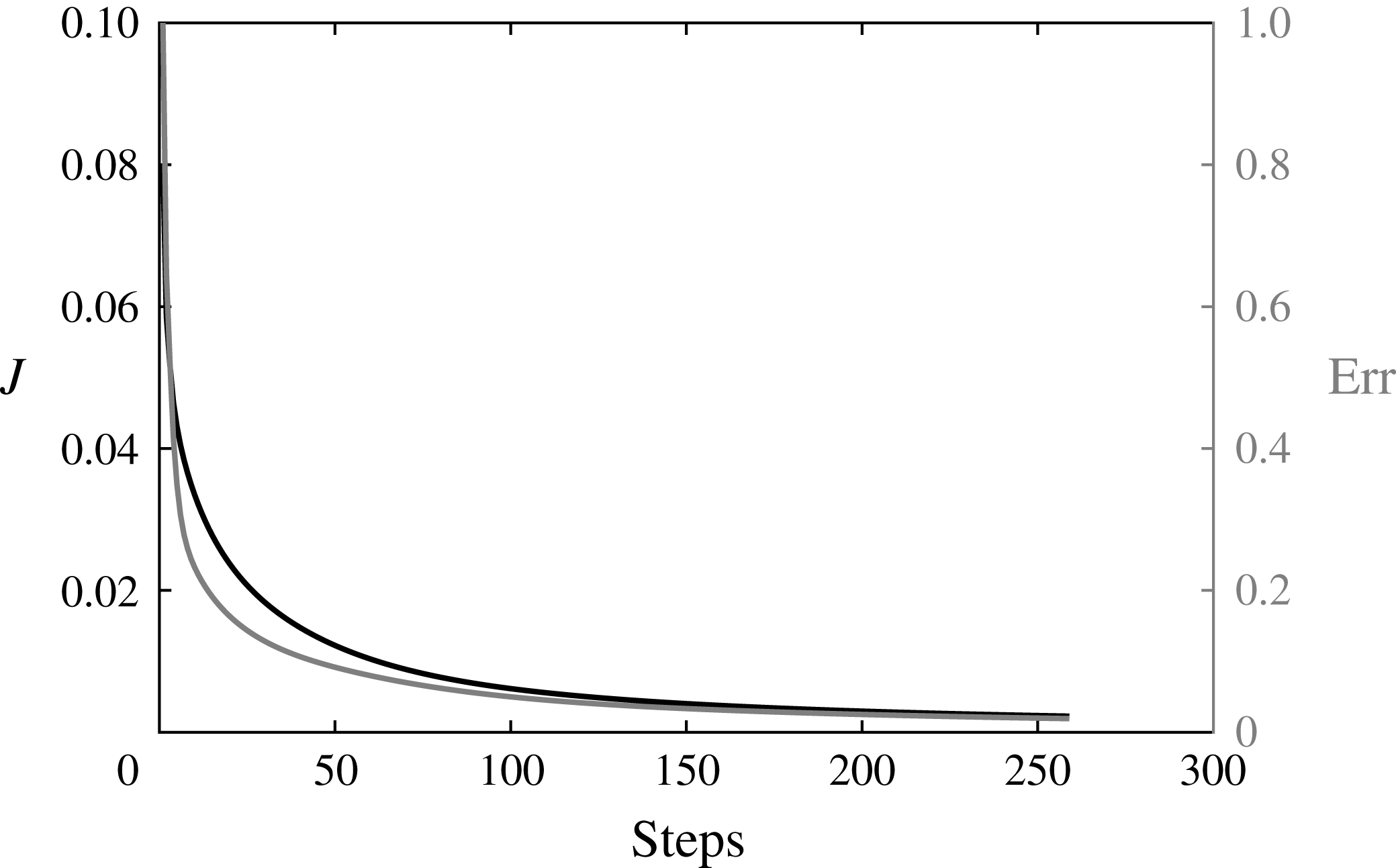
The optimal control problems are solved by a conjugate-gradient method where the direction is updated by a Polak & Ribiere (Reference Polak and Ribiere1969) method and the step length is defined by an Armijo line search method, see Polak (Reference Polak1997). The initial step
 $\unicode[STIX]{x1D70F}$
is dependent on the flow case and has been chosen to ensure convergence (see § B.2) and the control weight is set to
 $\unicode[STIX]{x1D6FC}=10^{-5}$
. Since the ‘base flow stabilization’ is a non-convex problem, the solution invariance was checked with respect to the parameter
 $\unicode[STIX]{x1D6FC}$
, the initial step lengths and the optimization methods. The results are presented in § B.2, where the solution has been found to be quasi-invariant under these choices in the methods.
The optimization algorithms for the ‘flow manipulation control’ and the ‘base flow stabilization control’ have been solved numerically with Freefem++ software in the same spirit as the base flow and eigenvalue problem computations. The same mesh and discretization technique are applied. In the case of the ‘mean flow stabilization control’, the time-averaged flow field is computed by DNS in NEK5000 before being transferred on the axisymmetric mesh. The other minimization steps of the conjugate-gradient algorithm are computed within Freefem++ until the next updated control (updated volume force) is obtained and returned to the 3-D DNS. The optimization process is stopped when the objective function
 ${\mathcal{J}}$
reaches a minimum, see § B.2.
5 Flow control results
5.1 Base flow manipulation control at
 $Re=180$

The predictive control of the axisymmetric bubble base flow minimizing the quadratic objective function equation (4.1) at
 $Re=180$
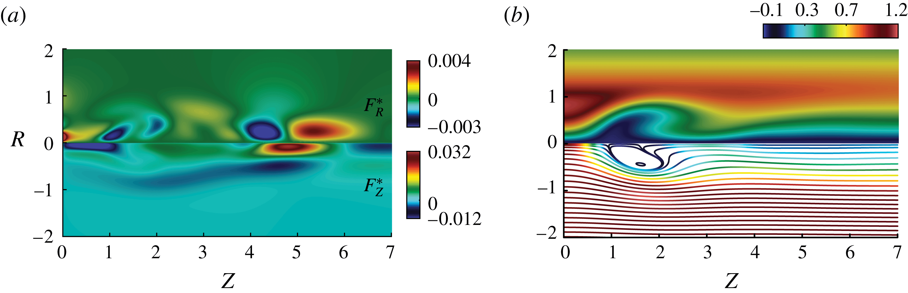
is displayed through the associated volume forcing in figure 8(a) and the flow solution
 $\boldsymbol{V}^{\ast }$
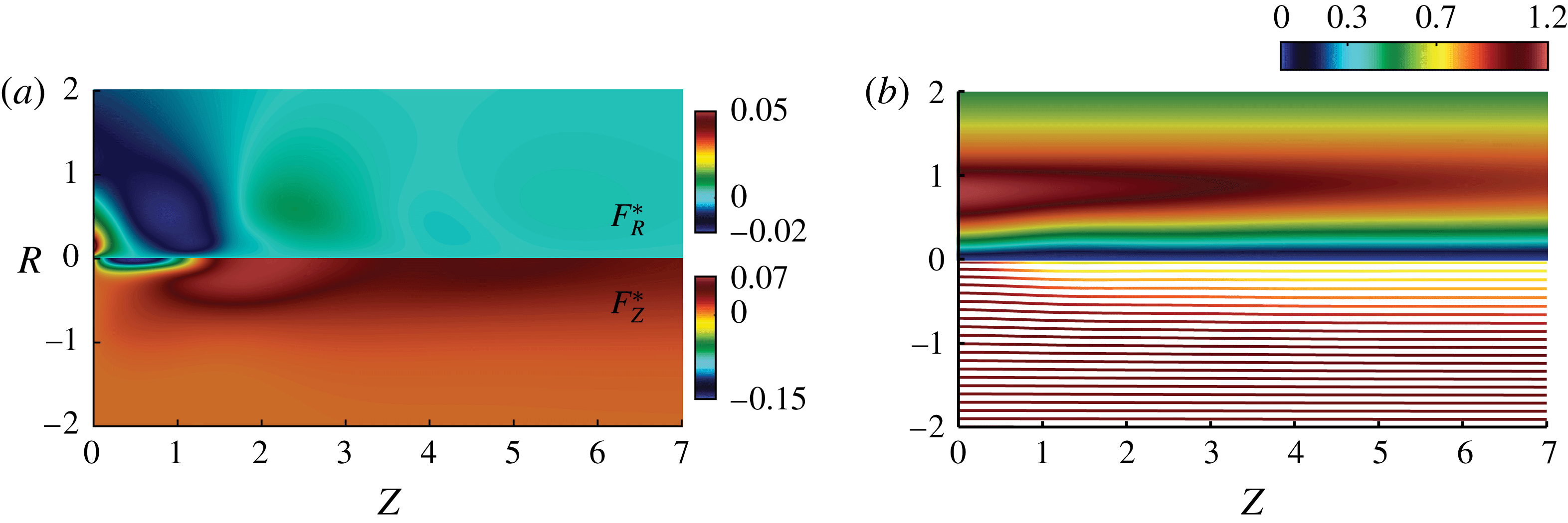
in figure 8(b). The radial velocity component exhibited by the streamsurfaces is clearly reduced by the minimization algorithm, starting with a maximum value of
 $V_{R}^{max}=0.3$
and ending with a value of
 $V_{R}^{max}=0.037$
at convergence, leading to a columnar solution contrasting with the uncontrolled bubble breakdown, see figure 5(a). Although the control target is not the recirculation bubble itself (in contrast to what was proposed in Boujo & Gallaire (Reference Boujo and Gallaire2014) for plane flows) or the recirculation intensity, we note that the use of our physical mechanism inspired surrogate objective entirely suppresses the recirculation: the minimum centreline axial velocity evolves from an uncontrolled value of
 $V_{Z}^{min}=-0.08$
to a controlled value of
 $V_{Z}^{min}=0.8$
. The volume force needed to restore a breakdown-free columnar solution is a predominating axial suction upstream of the nominal breakdown bubble combined with a subdominant radial correction, see figure 8(a), both resulting in a control amplitude at convergence of
 $\Vert \boldsymbol{F}^{\ast }||=0.084$
, see figure 18 in § B.2.
Navier–Stokes solutions for the base flow manipulation control at
 $Re=180$
(b) and the associated volume force (a) at the minimum of the functional
 ${\mathcal{J}}_{Manip}$
. The upper part of the graph (b) shows the tangential velocity component and the lower part, the streamsurfaces coloured by the magnitude of the axial velocity component.

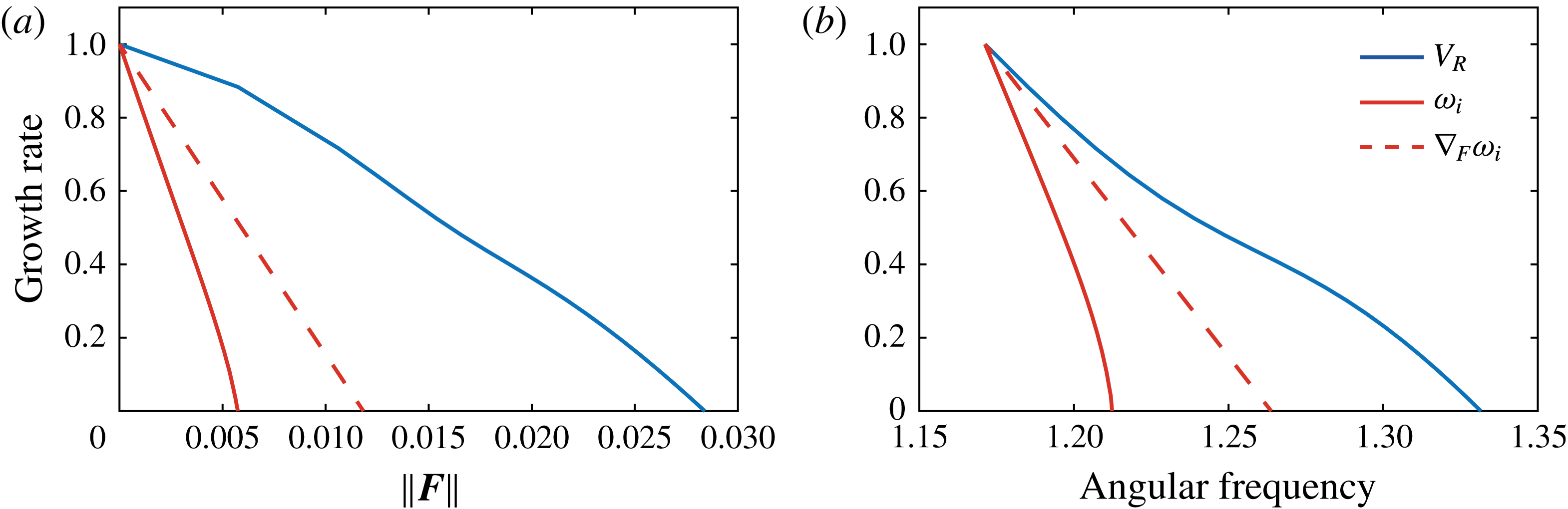
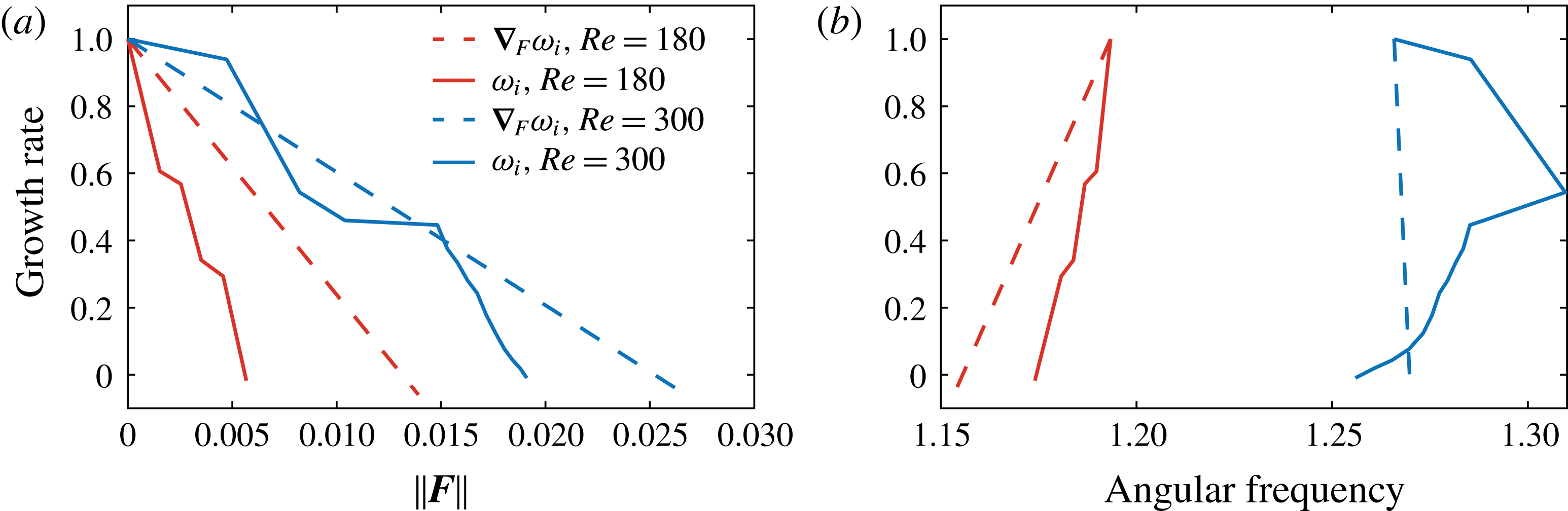
We have verified that the suppression of the recirculation bubble results in the stabilization of the spiral mode, as anticipated by the understanding of the underlying physical mechanism. Figure 9(a) (blue solid curve) demonstrates that the stabilization is achieved for a control amplitude of
 $\Vert \boldsymbol{F}\Vert =0.028$
, far beyond the minimizing control amplitude
 $\Vert \boldsymbol{F}^{\ast }\Vert =0.084$
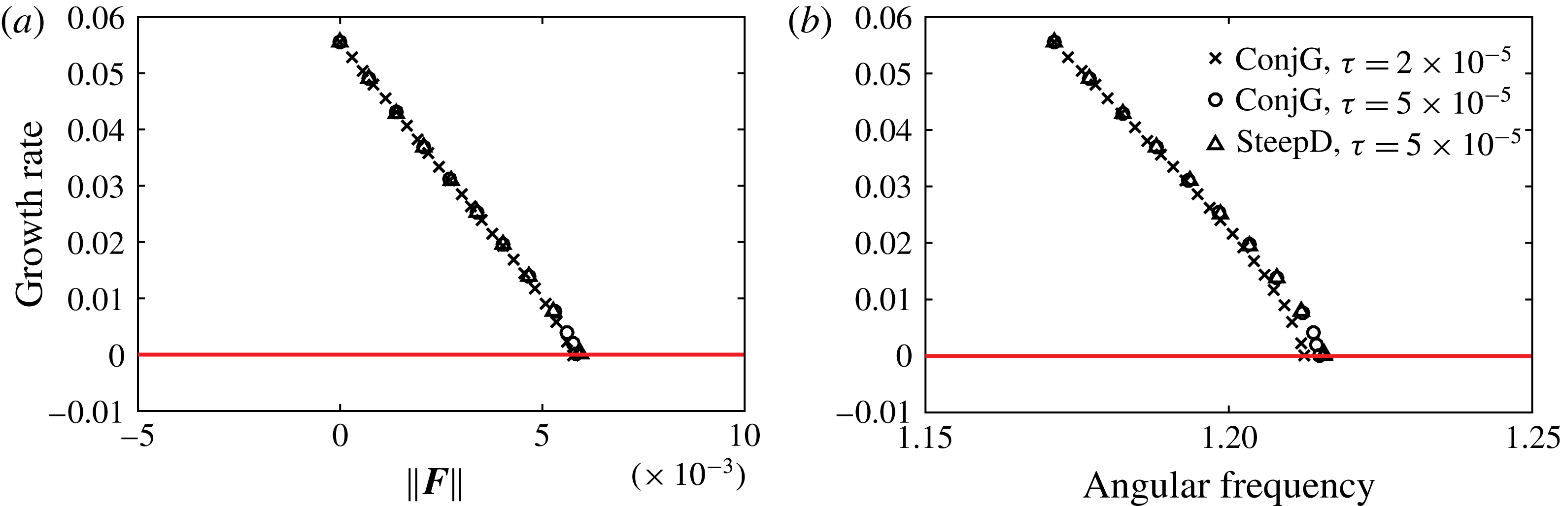
. Note that this stabilization is accompanied by a 10 % frequency shift (see the blue solid curve in figure 9
b). While physically well motivated the ‘flow manipulation control’ will appear as suboptimal when compared to the ‘flow stabilization control’ presented in § 5.2. As we will see, the comparison of figures 8(a) and 10(a) will show that a lot of control authority is spent in reducing the radial velocity in regions of low receptivity of the instability. We therefore now turn our efforts to base flow stabilization control, trading the conservative but quadratic cost functional (4.1) for a more precise but non-convex cost functional (4.2).
5.2 Base flow stabilization control at
$Re=180$

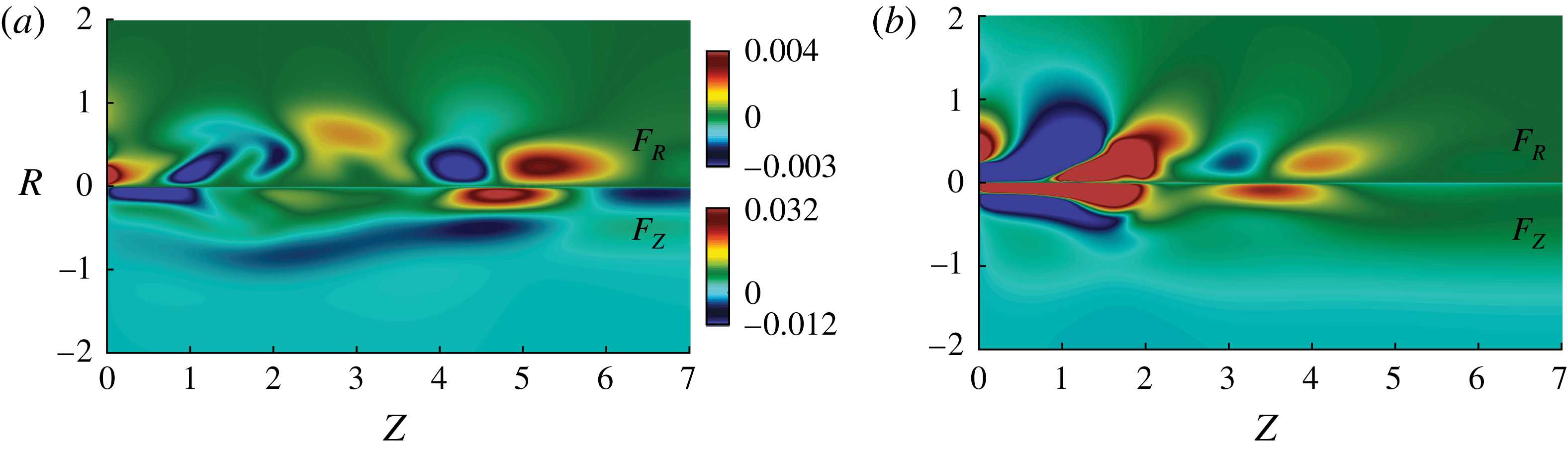
Despite the absence of mathematical proof, we have observed that the minimization algorithm targeting the eigenvalue growth rate of the spiral vortex breakdown mode developing on the base flow, herein referred to as ‘base flow stabilization control’, succeeds in stabilizing the flow. As seen by the red solid curve in figure 9(a), the normalized eigenvalue growth rate progressively decreases until stabilization for
 $\Vert \boldsymbol{F}^{\ast }\Vert =0.0058$
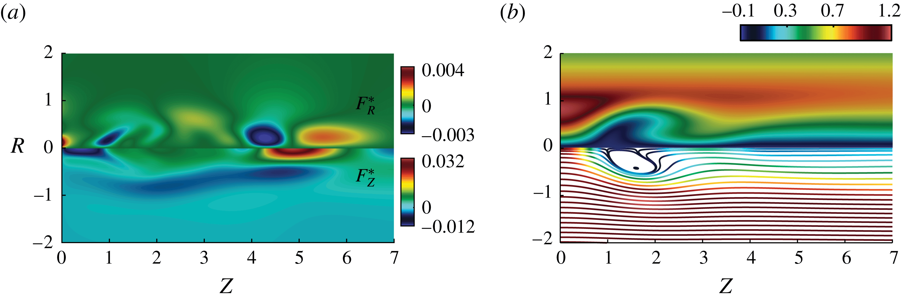
, i.e. 5 times less than the ‘flow manipulation control’ approach. Interestingly, a finite amplitude recirculation bubble is still present in the stable, optimally controlled flow reported in figure 10(b). The comparison with the uncontrolled base flow (see figure 5
a) shows that minimal changes in the recirculation bubble are sufficient to restore the stability of the flow and this stabilization goes together with a small frequency shift, reported in figure 9(b).
Base flow dominant growth rate normalized by the most unstable uncontrolled eigenvalue at
 $Re=180$
as a function of the norm of the control (a) and of the angular frequency of the mode (b) for the ‘flow manipulation control’ (blue solid curve) and ‘base flow stabilization control’ (red solid curve), and the ‘linear sensitivity-based finite amplitude control’ (red dashed curve).

Optimal ‘base flow stabilization control’ force (a) and associated flow solution (b) at
 $Re=180$
and
 $S=1.095$
. The upper part of the graph (b) shows the tangential velocity component and the lower part, the streamsurfaces coloured by the magnitude of the axial velocity component.

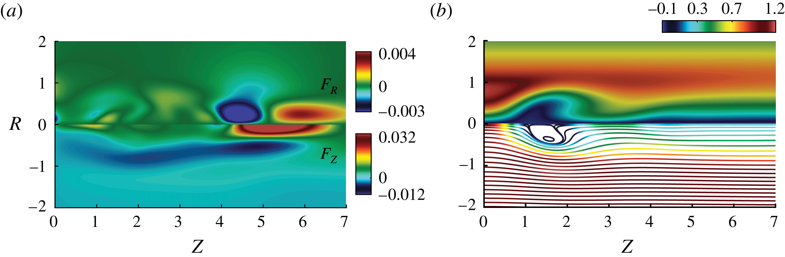
The determination of this optimal, nonlinear, predictive control requires a computationally expensive iterative minimization procedure. A linear sensitivity-based finite amplitude control therefore provides a promising alternative. The latter is included in the red dashed curve in figure 9(a), showing that, although linearity is preserved, flow stabilization is achieved for approximately two times more control amplitude. A comparison of both volume force distributions in figures 10(a) and 11(a) shows in addition that the first gradient direction may deviate quite substantially from the nonlinear optimal control. While the latter suggests to decelerate the flow in the inlet region, thereby pulling on the recirculation bubble, the sensitivity-based centreline axial force accelerates the flow upstream of the bubble, thereby pushing the bubble downstream. This results in slightly different flow topologies (see figures 10
b and 11
b), noting that in both cases, the bubble is slightly smaller than in the nominal, unstable, base flow reported in figure 5(a). In contrast, the volume forces acting in bubble wake around
 $Z=5$
are very similar and act to accelerate the flow in the wake region. This is also clearly visible from the resulting controlled flows (figures 10
b and 11
b) when compared to the base flow (figure 5
a). All these results illustrate that, even for moderate growth rates, the finite amplitude linear sensitivity to a steady force can remain significantly suboptimal. We now turn our attention to the mean flow stabilization control, first at
 $Re=180$
.
Suboptimal ‘linear sensitivity-based finite amplitude control’ (a) and associated flow solution (b) at
 $Re=180$
and
 $S=1.095$
. The upper part of the graph (b) shows the tangential velocity component and the lower part, the streamsurfaces coloured by the magnitude of the axial velocity component.

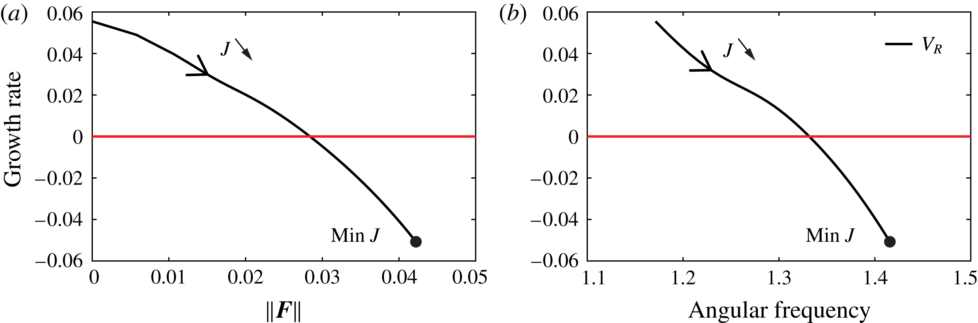
Mean flow dominant growth rate, normalized by the most unstable uncontrolled mean flow eigenvalue at
 $Re=180$
(red curves) and
 $Re=300$
(blue curves) as a function of the norm of the control (a) and of the angular frequency of the mode (b) for the nonlinear mean flow stabilization (solid curves) and the ‘linear sensitivity-based finite amplitude control’ (dashed curves).

5.3 Mean flow stabilization at
$Re=180$

The control magnitude and eigenvalue path during the minimization process are exhibited in solid red lines in figure 12(a,b) for the ‘mean flow stabilization control’ at
 $Re=180$
, together with the ‘linear sensitivity-based finite amplitude control’ of the mean flow (red dashed lines). The optimal mean flow stabilization control is reached for a norm of
 $\Vert \boldsymbol{F}^{\ast }\Vert =0.0057$
while the linear sensitivity-based finite amplitude control stabilizes the flow for
 $\Vert \boldsymbol{F}^{\ast }\Vert =0.014$
. These values compare very well with those obtained for the base flow stabilization control. The volume force and controlled solution, see figure 13, are also very similar to those of the base flow control, see figure 10. This indicates the consistency of both approaches targeting the dominant growth rate of the mean and base flows respectively, for parameters close to the bifurcation threshold, even if the least unstable eigenvalues of the base and mean flow differ by a factor 10. The 3-D vorticity contour of the controlled flow solution is plotted in figure 16(a), demonstrating that the axisymmetry of the flow is restored and the inspection of the time-dependent traces remains stationary.
Time-averaged 3-D Navier–Stokes solution of the mean flow stabilization control (b) and the related force applied (a) for
 $Re=180$
at convergence. The upper part of the graph (b) shows the tangential velocity component and the lower part, the streamsurfaces coloured by the magnitude of the axial velocity component.

The linear sensitivity-based finite amplitude control about the mean flow is presented in figure 14(a) and represents the initial sensitivity to a steady force for
 $Re=180$
. The receptivity distribution, while suboptimal, is very similar to the nonlinear sensitivity map, and enables a correct identification of the maximum and minimum locations.
Suboptimal ‘linear sensitivity-based finite amplitude control’ about the mean flow at
 $Re=180$
(a) and
 $Re=300$
(b) for a swirl number of
 $S=1.095$
.

5.4 Mean flow stabilization at
$Re=300$

At
 $Re=300$
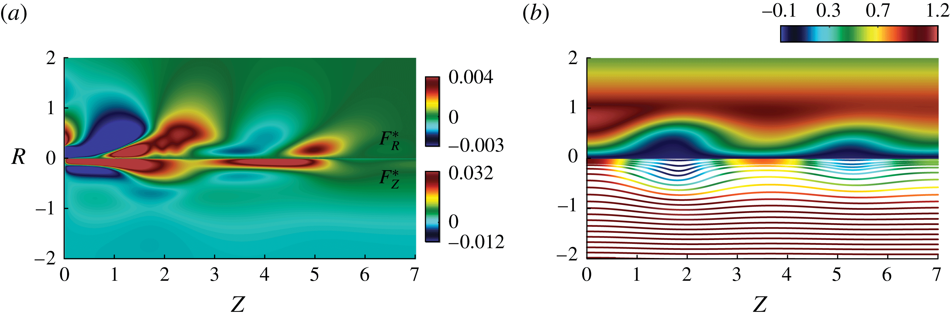
, the minimization path is less straight, and the optimal solution (solid blue line in figure 12) seems to oscillate around the trajectory of the ‘linear sensitivity-based finite amplitude control’ (dashed blue line in figure 12) before eventually sensibly reducing the eigenvalue growth rate at the end of the algorithm. The control magnitude is
 $\Vert \boldsymbol{F}^{\ast }\Vert =0.019$
at convergence, to be compared with the value of
 $\Vert \boldsymbol{F}^{\ast }\Vert =0.027$
required for the mean flow ‘linear sensitivity-based finite amplitude control’. The optimal volume force as well as the resulting controlled flow solution are exhibited in figure 15. In contrast to the Reynolds number
 $Re=180$
case, most of the control effort is located in the recirculating bubble region while little forcing acts in the wake region. The upstream forcing blows the bubble downstream, as opposed to the optimal forcing at
 $Re=180$
, where the bubble was sucked. The controlled flow solution has no recirculation, but adopts instead a wavy form and demonstrates therefore that a large modification of the mean flow is required to restore its stability, while a small modification is required at a Reynolds value of
 $Re=180$
. The 3-D solution is displayed in figure 16(b), demonstrating the axisymmetrization of the controlled flow. Although several waves are observed on the vorticity contour, we have checked that the controlled flow remains steady. In addition, the ‘linear sensitivity-based finite amplitude control’ about the mean flow is presented in figure 14(b) and represents the initial sensitivity to a steady force for
 $Re=300$
. Similarly to the ‘mean flow stabilization control’ at a Reynolds value of
 $Re=180$
, the linear receptivity well identifies the maximum and minimum of the nonlinear receptivity map (see figure 15
a), although it remains suboptimal (see figure 12).
Time-averaged 3-D Navier–Stokes solution of the mean flow stabilization control (b) and the related force applied (a) for
 $Re=300$
at convergence. The upper part of the graph (b) shows the tangential velocity component and the lower part, the streamsurfaces coloured by the magnitude of the axial velocity component.


6 Discussion and conclusion
In this study, we have first discussed the validity of the base flow and mean flow stability analyses in predicting the frequency of the self-sustained single spiral vortex breakdown mode appearing for sufficient swirl and Reynolds numbers in the flow geometry of Ruith et al. (Reference Ruith, Chen, Meiburg and Maxworthy2003). Fixing the swirl number to
 $S=1.095$
, we have seen that the two stability analyses coincide with the limit cycle frequency close to the bifurcation threshold until
 $Re\sim 200$
. For larger Reynolds number, the mean flow stability analysis provides an excellent prediction of the dominant frequency in the nonlinear simulations, in contrast to the base flow stability analysis, as the consequence of an important mean flow modification: while the base flow has two recirculation bubbles at
 $Re=300$
, the mean flow has only one much smaller recirculation bubble. This result emphasizes the successful prediction provided by the stability analysis around the mean flow, which was also recently reported for turbulent mean flow in industrial applications (Oberleithner et al.
Reference Oberleithner, Sthr, Im, Arndt and Steinberg2015; Paredes et al.
Reference Paredes, Terhaar, Oberleithner, Theofilis and Passchereit2015; Tammisola & Juniper Reference Tammisola and Juniper2016; Pasche et al.
Reference Pasche, Avellan and Gallaire2017). Moreover in the present study, we observe a second unstable global mode above a Reynolds value of
 $Re=300$
. This second instability should be interpreted in light of the self-consistent model for saturation dynamics of self-sustained instabilities (Mantič-Lugo et al.
Reference Mantič-Lugo, Arratia and Gallaire2014).
We have then investigated the predictive control of the spiral vortex breakdown based on adjoint optimization method. The spiral vortex breakdown was quenched by an axisymmetric steady volume force distribution on
 $(\boldsymbol{e}_{R},\boldsymbol{e}_{Z})$
obtained by minimizing two different objective functions, a non-convex objective function targeting the most unstable eigenvalue growth rate of the base or mean flow stability analyses, that directly acts on the instability marker (‘flow stabilization control’) and a quadratic objective function minimizing the norm of the radial velocity distribution that is inspired by the physical mechanism governing spiral vortex breakdown (‘flow manipulation control’). These control strategies were computed in an axisymmetric domain avoiding expensive 3-D minimization computations. This dimensionality reduction from the 3-D domain to a 2-D axisymmetric domain is performed thanks to the azimuthal Fourier decomposition naturally appearing in the eigenvalue analysis involved in the ‘flow stabilization control’. We can therefore expect to tackle self-sustained instability control at larger Reynolds numbers. The gradient direction involved in the minimization of the ‘flow stabilization control’ uses the linear sensitivity to a steady force (Giannetti & Luchini Reference Giannetti and Luchini2007; Marquet et al.
Reference Marquet, Sipp and Jacquin2008) at each iteration step. A simpler approach has also been followed where the first gradient direction is chosen and only the amplitude varied referred to as ‘linear sensitivity-based finite amplitude control’.
The ‘flow manipulation control’ succeeded in stabilizing the flow at
 $Re=180$
, at the price of a significant control cost. This surrogate control was found suboptimal in contrast to the ‘flow stabilization control’ but the direction of the volume force upstream of the bubble is identical and pulls on the recirculation bubble. The ‘linear sensitivity-based finite amplitude control’ was also found to be successful but suboptimal. While the force distribution was correct in the vortex breakdown bubble wake, its sign was opposite to the optimal stabilization control upstream of the bubble, demonstrating the fragility of this computationally cheaper method.
The control of the mean flow was found equivalent to the base flow control at
 $Re=180$
. Both yielded a controlled flow preserving its recirculation bubble. The same control norm and force distribution are found for the base and mean flow control, while the growth rate differs by a factor of 10 between the base and mean eigenvalue, showing the consistency of the base and mean flow eigenvalues control. This result emphasizes the non-neutrality of the eigenvalue growth rate and its practical usefulness in applying such control strategies. This encouraged us to explore the mean flow stabilization control at a much larger Reynolds number of
 $Re=300$
. Targeting only the dominant mean flow growth rate, the optimal control was found to be successful in quenching all spiral modes for a control cost four times higher than at
 $Re=180$
, yielding a controlled flow solution where recirculation regions were quenched by a volume force pushing the bubble downstream. The ‘linear sensitivity-based finite amplitude control’ was also found to be successful, although suboptimal.
This also suggests this technique may be used to stabilize instabilities prevailing in a turbulent background, i.e. in turbulent flows dominated by a self-sustained periodic instability, by using the sensitivity computed by Meliga et al. (Reference Meliga, Pujals and Serre2012b
) for turbulent flows. In the context of spiral vortex breakdown, a natural extension of the present work is the control of the precessing vortex rope in Francis turbines operating at off-design conditions Pasche (Reference Pasche2018). While the finite amplitude volume force projected on the radial and axial component may appear to be a pure theoretical concept, it can be in principle practically realized by an axisymmetric appendage to control the flow without external energy or it can be used as a design step to access the most receptive region of the instability by applying blowing or suction along a suitable region. Alternatively the present control strategy can be generalized to boundary control. First attempts (not shown) indicate that the instability can be quenched successfully at Reynolds
 $Re=180$
by pure radial inlet injection. This result contrasts with the distributed control, which shows a larger contribution of the axial component (figure 13). Turning back to distributed control, we underline the correct identification by the mean flow based linear sensitivity map of the minimum and maximum of the nonlinear receptivity regions, both close to the threshold
 $Re=180$
and far away from it
 $Re=300$
. Linear sensitivity maps may therefore be sufficient to develop an appendage accessing these locations, although their validity cannot be ensured a priori. Optimal nonlinear sensitivity maps, as developed in this study, appear therefore as the most consistent and promising approach for industrial applications (Paredes et al.
Reference Paredes, Terhaar, Oberleithner, Theofilis and Passchereit2015; Pasche Reference Pasche2018).
Acknowledgements
The authors are grateful to the Swiss National Science Foundation (grant no. 200021 149818.1) which has supported this work.
Appendix A. Validation and convergence studies
A.1 Validation of the 3-D DNS
The 3-D direct numerical flow simulations have been validated by changing the mesh size, the mesh topology, the boundary conditions, the domain dimensions and the time step for a fixed swirl number
 $S=1.095$
and Reynolds number
 $Re=200$
. The convergence criteria are based on the deviation of the frequency and the amplitude of the radial velocity component of the single helical vortex flow. These values are monitored at
 $(R,\unicode[STIX]{x1D703},Z)=(0.1,0.0,5.0)$
which is located after the bubble, in the helical flow region. The results of this convergence study are displayed on table 2. The topology of the mesh is an O-grid type with two different cell arrangements in the centre: diamond cells that almost preserve the azimuthal symmetry of the problem and square cells. All cells have a
 $P_{10}$
and
 $P_{8}$
spectral discretizations with a uniform number of nodes
 $n_{x}\times n_{y}\times n_{z}=10\times 10\times 10$
and
 $n_{x}\times n_{y}\times n_{z}=8\times 8\times 8$
for velocities and pressure respectively. The robustness of the solutions with respect to the convective boundary condition on the outlet
 $\unicode[STIX]{x1D6E4}_{out}$
is investigated by changing the length of the reference domain to
 $Z_{max}=60$
for mesh M6 instead of
 $Z_{max}=40$
. The radial unconfinement is guaranteed by the invariance in regard to the lateral boundary conditions (free outflow or no slip). The Courant–Friedrichs–Lewy (CFL) number invariance is also investigated on the mesh M9 and finally a refined mesh M7 concludes the convergence analysis. In the present study the mesh M5 is the reference mesh for the results presented.
Convergence of the 3-D numerical flow simulations and eigenvalues of mean flow for
 $Re=200$
,
 $S=1.095$
.

A.2 Eigenvalue convergence of the base flow
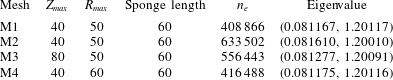
The mesh of the axisymmetric domain is designed in a way that the convergence of the most unstable eigenvalue is obtained when solving the eigenvalue problem related to (2.6). Therefore different domain sizes and meshes have been investigated, and the values of the most eigenvalue are resumed on table 3. The mesh M1 has been selected for the present study and the same mesh is used for the base flow computation.
Eigenvalue sensitivity to the mesh configuration for
 $Re=200$
,
 $S=1.095$
.

A.3 Eigenvalue convergence of the mean flow
The mesh designed for the eigenvalue problem of the base flow is kept for the eigenvalue problem of the mean flow except that the sponge region is removed. The domain without the sponge region exactly fits the 3-D domain avoiding the need for an extrapolation procedure. A spectral interpolation is solely required to transfer the time-averaged flow field to the axisymmetric velocity space. We have to mention that the convective boundary condition at the outlet of the 3-D domain is replaced by a free-outflow condition at the outlet of the axisymmetric domain. This does not have any impact on the convergence of the eigenvalues, as supported by the invariance of the eigenvalue with respect to the length of the 3-D domain (see the last column of table 2). For the reference mesh M5, the refined mesh M7 and the longer domain mesh M6, both the frequency and the growth rates of the eigenvalues are similar.
Appendix B. Optimal control problem
B.1 Optimal control theory
The formalism of the optimal control problem for the ‘flow manipulation control’ and the ‘flow stabilization control’ is introduced in this appendix. Our aim is to solve the following general constrained minimization problem:
 $$\begin{eqnarray}\displaystyle \left.\begin{array}{@{}c@{}}\text{find}\quad \boldsymbol{F}\in {\mathcal{U}},\quad \boldsymbol{F}=\text{min}\,{\mathcal{J}}(\boldsymbol{F},\boldsymbol{V})\quad \text{with}\\ (\boldsymbol{V}\boldsymbol{\cdot }\unicode[STIX]{x1D735})\boldsymbol{V}=-\unicode[STIX]{x1D735}P+Re^{-1}\unicode[STIX]{x1D6FB}^{2}\boldsymbol{V}+\boldsymbol{F}\quad \text{in}~\unicode[STIX]{x1D6FA}_{a}\\ \unicode[STIX]{x1D735}\boldsymbol{\cdot }\boldsymbol{V}=0\quad \text{in}~\unicode[STIX]{x1D6FA}_{a}\\ -\text{i}\unicode[STIX]{x1D714}\boldsymbol{v}+(\boldsymbol{V}\boldsymbol{\cdot }\unicode[STIX]{x1D735})\boldsymbol{v}+(\boldsymbol{v}\boldsymbol{\cdot }\unicode[STIX]{x1D735})\boldsymbol{V}=-\unicode[STIX]{x1D735}p+Re^{-1}\unicode[STIX]{x1D6FB}^{2}\boldsymbol{v}\quad \text{in}~\unicode[STIX]{x1D6FA}_{a}\\ \unicode[STIX]{x1D735}\boldsymbol{\cdot }\boldsymbol{v}=0\quad \text{in}~\unicode[STIX]{x1D6FA}_{a}\\ G(\boldsymbol{V})=0\quad \text{on}~\unicode[STIX]{x1D6E4}\\ g(\boldsymbol{v})=0\quad \text{on}~\unicode[STIX]{x1D6E4},\end{array}\right\} & & \displaystyle\end{eqnarray}$$
where
 ${\mathcal{J}}$
is the objective function,
 $(\boldsymbol{V},P)\in {\mathcal{V}}$
the state variables,
 $\boldsymbol{F}$
the control variable,
 $(\boldsymbol{v},p)$
the global eigenmodes,
 $\unicode[STIX]{x1D6FA}$
the domain,
 $\unicode[STIX]{x1D6E4}$
the boundaries of the domain,
 $G$
and
 $g$
the associated boundary conditions and
 ${\mathcal{V}}$
and
 ${\mathcal{U}}$
two Hilbert spaces.
We consider first the ‘flow manipulation problem’ for a distributed control, the objective function of which reads:
 $$\begin{eqnarray}{\mathcal{J}}_{Manip}(\boldsymbol{F})=\frac{1}{2}\int \!\!\!\int _{\unicode[STIX]{x1D6FA}_{a}}\Vert \boldsymbol{V}(\boldsymbol{F})-\boldsymbol{z}_{\boldsymbol{d}}\Vert ^{2}\,\text{d}\unicode[STIX]{x1D6FA}_{a}+\frac{\unicode[STIX]{x1D6FC}}{2}\int \!\!\!\int _{\unicode[STIX]{x1D6FA}_{a}}\Vert \boldsymbol{F}\Vert ^{2}\,\text{d}\unicode[STIX]{x1D6FA}_{a},\end{eqnarray}$$
with
 $\boldsymbol{z}_{\boldsymbol{d}}=\mathbf{0}$
,
 $\boldsymbol{V}=(V_{R},0,0)$
and
 $\boldsymbol{F}=(F_{R},0,F_{Z})$
. This objective function targets a minimal radial velocity component controlled by radial and axial distributed volume forces. Since we have defined the objective function, the associated Lagrangian functional with respect to the governing equations is expressed as
 $$\begin{eqnarray}\displaystyle {\mathcal{L}}([\boldsymbol{V},P],\boldsymbol{F},[\boldsymbol{V}^{\dagger },P^{\dagger }]) & = & \displaystyle {\mathcal{J}}(\boldsymbol{V},\boldsymbol{F})-a(\boldsymbol{V},\boldsymbol{V}^{\dagger })-c(\boldsymbol{V},\boldsymbol{V},\boldsymbol{V}^{\dagger })\nonumber\\ \displaystyle & & \displaystyle -\,b(\boldsymbol{V}^{\dagger },P)-b(\boldsymbol{V},P^{\dagger })+(\boldsymbol{F},\boldsymbol{V}^{\dagger }),\end{eqnarray}$$
where
 $a(.,.)$
,
 $b(.,.)$
are the bilinear form of the viscous, pressure and divergence,
 $(.,.)$
is the Hermitian inner product,
 $c(.,.,.)$
is the trilinear form and
 $(\boldsymbol{V}^{\dagger },P^{\dagger })$
are the Lagrange multipliers, also called adjoint variables. Observe that the eigenvalue equation does not appear in this Lagrangian, since it is not a control target, as we manipulate the base flow by targeting the radial velocity intensity as a proxy for flow non-parallelism. The distinct set of equations systems solved in the minimization problem are derived by satisfying the first-order optimal condition of the Lagrangian, according to
 $$\begin{eqnarray}\left.\frac{\text{d}}{\text{d}_{\unicode[STIX]{x1D716}}}{\mathcal{L}}([\cdots +\unicode[STIX]{x1D716}\unicode[STIX]{x1D719}])\right|_{\unicode[STIX]{x1D716}=0}=0.\end{eqnarray}$$
This condition is computed by the Frechet derivative, where
 $\unicode[STIX]{x1D719}\in {\mathcal{V}}$
is the test function associated with each variable and leads to the state equations, the adjoint problem and the optimality condition. These systems of equations are expressed in strong form with the boundary conditions related to our problem in (B 5)–(B 7).
State equations:
 $$\begin{eqnarray}\left.\begin{array}{@{}c@{}}\unicode[STIX]{x1D735}\boldsymbol{V}\boldsymbol{\cdot }\boldsymbol{V}=-\unicode[STIX]{x1D735}P+Re^{-1}\unicode[STIX]{x1D6FB}^{2}\boldsymbol{V}+\boldsymbol{F}\quad \text{in}~\unicode[STIX]{x1D6FA}_{a}\\ \unicode[STIX]{x1D735}\boldsymbol{\cdot }\boldsymbol{V}=0\quad \text{in}~\unicode[STIX]{x1D6FA}_{a}\\ V_{R}(R)=0,\quad V_{\unicode[STIX]{x1D703}}(R)=S\unicode[STIX]{x1D6F9},\quad V_{Z}(R)=1\quad \text{on}~\unicode[STIX]{x1D6E4}_{in}\\ V_{R}=V_{\unicode[STIX]{x1D703}}=\unicode[STIX]{x2202}_{R}V_{Z}=0\quad \text{on}~\unicode[STIX]{x1D6E4}_{axis}\\ Re^{-1}\unicode[STIX]{x2202}_{\boldsymbol{n}}\boldsymbol{V}-P\boldsymbol{n}=0\quad \text{on}~\unicode[STIX]{x1D6E4}_{ext},\unicode[STIX]{x1D6E4}_{out}\end{array}\right\}\end{eqnarray}$$
Adjoint equations:
 $$\begin{eqnarray}\left.\begin{array}{@{}c@{}}\unicode[STIX]{x1D735}^{T}\boldsymbol{V}\boldsymbol{\cdot }\boldsymbol{V}^{\dagger }-\unicode[STIX]{x1D735}\boldsymbol{V}^{\dagger }\boldsymbol{\cdot }\boldsymbol{V}=-\unicode[STIX]{x1D735}P^{\dagger }+Re^{-1}\unicode[STIX]{x1D6FB}^{2}\boldsymbol{V}^{\dagger }+\boldsymbol{V}-\boldsymbol{z}_{\boldsymbol{d}}\quad \text{in}~\unicode[STIX]{x1D6FA}_{a}\\ \unicode[STIX]{x1D735}\boldsymbol{\cdot }\boldsymbol{V}^{\dagger }=0\quad \text{in}~\unicode[STIX]{x1D6FA}_{a}\\ \boldsymbol{V}^{\dagger }=0\quad \text{on}~\unicode[STIX]{x1D6E4}_{in}\\ V_{R}^{\dagger }=V_{\unicode[STIX]{x1D703}}^{\dagger }=\unicode[STIX]{x2202}_{R}V_{Z}^{\dagger }=0\quad \text{on}~\unicode[STIX]{x1D6E4}_{axis}\\ Re^{-1}\unicode[STIX]{x2202}_{\boldsymbol{n}}\boldsymbol{V}^{\dagger }-P^{\dagger }\boldsymbol{n}+(\boldsymbol{V}\boldsymbol{\cdot }\boldsymbol{n})\boldsymbol{V}^{\dagger }=0\quad \text{on}~\unicode[STIX]{x1D6E4}_{ext},\unicode[STIX]{x1D6E4}_{out}\end{array}\right\}\end{eqnarray}$$
Optimality condition:
 $$\begin{eqnarray}\unicode[STIX]{x1D735}{\mathcal{J}}=\boldsymbol{V}^{\dagger }+\unicode[STIX]{x1D6FC}\boldsymbol{F}.\end{eqnarray}$$
As highlighted in the body of the paper, the main advantage of this flow manipulation control approach is to ensure a quadratic objective function.
We next consider the direct so-called ‘flow stabilization control’ problem for a distributed control, the objective function of which reads:
 $$\begin{eqnarray}{\mathcal{J}}_{Stab}(\boldsymbol{F})=|\text{Im}(\unicode[STIX]{x1D714})|+\frac{\unicode[STIX]{x1D6FC}}{2}\int \!\!\!\int _{\unicode[STIX]{x1D6FA}_{a}}\Vert \boldsymbol{F}\Vert ^{2}\,\text{d}\unicode[STIX]{x1D6FA}_{a}.\end{eqnarray}$$
The Lagrangian functional of this minimization problem is expressed as:
 $$\begin{eqnarray}\displaystyle & & \displaystyle {\mathcal{L}}(\unicode[STIX]{x1D714},[\boldsymbol{v},p],[\boldsymbol{V},P],[\boldsymbol{v}^{\dagger },p^{\dagger }],[\boldsymbol{V}^{\dagger },P^{\dagger }],\boldsymbol{F})={\mathcal{J}}(\unicode[STIX]{x1D714},\boldsymbol{F})-t(\boldsymbol{v},\boldsymbol{v}^{\dagger })-a(\boldsymbol{v},\boldsymbol{v}^{\dagger })\nonumber\\ \displaystyle & & \displaystyle \qquad -\,c(\boldsymbol{v},\boldsymbol{V},\boldsymbol{v}^{\dagger })-c(\boldsymbol{V},\boldsymbol{v},\boldsymbol{v}^{\dagger })-b(\boldsymbol{v}^{\dagger },p)-b(\boldsymbol{v},p^{\dagger })-a(\boldsymbol{V},\boldsymbol{V}^{\dagger })-c(\boldsymbol{V},\boldsymbol{V},\boldsymbol{V}^{\dagger })\nonumber\\ \displaystyle & & \displaystyle \qquad -\,b(\boldsymbol{V}^{\dagger },P)-b(\boldsymbol{V},P^{\dagger })+(\boldsymbol{F},\boldsymbol{V}^{\dagger }),\end{eqnarray}$$
where
 $t(.,.)$
is the mass matrix of the time derivative including the eigenvalue
 $\unicode[STIX]{x1D714}$
. Following the same procedure as for the previous problem, the stationary point of the Lagrangian functional leads to a system of six equations, the state equation, the direct eigenvalue problem, the adjoint eigenvalue problem, a normalization condition, the adjoint problem and the optimality condition. These problems are expressed in strong form with the boundary conditions related to our study in (B 10)–(B 15).
State equations:
 $$\begin{eqnarray}\left.\begin{array}{@{}c@{}}\unicode[STIX]{x1D735}\boldsymbol{V}\boldsymbol{\cdot }\boldsymbol{V}=-\unicode[STIX]{x1D735}P+Re^{-1}\unicode[STIX]{x1D6FB}^{2}\boldsymbol{V}+\boldsymbol{F}\quad \text{in}~\unicode[STIX]{x1D6FA}_{a}\\ \unicode[STIX]{x1D735}\boldsymbol{\cdot }\boldsymbol{V}=0\quad \text{in}~\unicode[STIX]{x1D6FA}_{a}\\ V_{R}(R)=0,\quad V_{\unicode[STIX]{x1D703}}(R)=S\unicode[STIX]{x1D6F9},\quad V_{Z}(R)=1\quad \text{on}~\unicode[STIX]{x1D6E4}_{in}\\ V_{R}=V_{\unicode[STIX]{x1D703}}=\unicode[STIX]{x2202}_{R}V_{Z}=0\quad \text{on}~\unicode[STIX]{x1D6E4}_{axis}\\ Re^{-1}\unicode[STIX]{x2202}_{\boldsymbol{n}}\boldsymbol{V}-P\boldsymbol{n}=0\quad \text{on}~\unicode[STIX]{x1D6E4}_{ext},\unicode[STIX]{x1D6E4}_{out}\end{array}\right\}\end{eqnarray}$$
Direct eigenvalue equations:
 $$\begin{eqnarray}\left.\begin{array}{@{}c@{}}-\text{i}\unicode[STIX]{x1D714}\boldsymbol{v}+\unicode[STIX]{x1D735}_{m}\boldsymbol{v}\boldsymbol{\cdot }\boldsymbol{V}+\unicode[STIX]{x1D735}\boldsymbol{V}\boldsymbol{\cdot }\boldsymbol{v}=-\unicode[STIX]{x1D735}_{m}p+Re^{-1}\unicode[STIX]{x1D735}_{m}^{2}\boldsymbol{v}\quad \text{in}~\unicode[STIX]{x1D6FA}_{a}\\ \unicode[STIX]{x1D735}_{m}\boldsymbol{\cdot }\boldsymbol{v}=0\quad \text{in}~\unicode[STIX]{x1D6FA}_{a}\\ \boldsymbol{v}=0\quad \text{on}~\unicode[STIX]{x1D6E4}_{in}\\ \text{cf. table 1}\quad \text{on}~\unicode[STIX]{x1D6E4}_{axis}\\ Re^{-1}\unicode[STIX]{x2202}_{\boldsymbol{n}}\boldsymbol{v}-p\boldsymbol{n}=0\quad \text{on}~\unicode[STIX]{x1D6E4}_{ext},\unicode[STIX]{x1D6E4}_{out}\end{array}\right\}\end{eqnarray}$$
Adjoint eigenvalue equations:
 $$\begin{eqnarray}\left.\begin{array}{@{}c@{}}\text{i}\unicode[STIX]{x1D714}^{\ast }\boldsymbol{v}^{\dagger }+\unicode[STIX]{x1D735}_{m}^{T}\boldsymbol{V}\boldsymbol{\cdot }\boldsymbol{v}^{\dagger }-\unicode[STIX]{x1D735}_{m}\boldsymbol{v}^{\dagger }\boldsymbol{\cdot }\boldsymbol{V}=-\unicode[STIX]{x1D735}_{m}p^{\dagger }+Re^{-1}\unicode[STIX]{x1D735}_{m}^{2}\boldsymbol{v}^{\dagger }\quad \text{in}~\unicode[STIX]{x1D6FA}_{a}\\ \unicode[STIX]{x1D735}_{m}\boldsymbol{\cdot }\boldsymbol{v}^{\dagger }=0\quad \text{in}~\unicode[STIX]{x1D6FA}_{a}\\ \boldsymbol{v}^{\dagger }=0\quad \text{on}~\unicode[STIX]{x1D6E4}_{in}\\ \text{cf. table 1}\quad \text{on}~\unicode[STIX]{x1D6E4}_{axis}\\ Re^{-1}\unicode[STIX]{x2202}_{\boldsymbol{n}}\boldsymbol{v}^{\dagger }-p^{\dagger }\boldsymbol{n}+(\boldsymbol{V}\boldsymbol{\cdot }\boldsymbol{n})\boldsymbol{v}^{\dagger }=0\quad \text{on}~\unicode[STIX]{x1D6E4}_{ext},\unicode[STIX]{x1D6E4}_{out}\end{array}\right\}\end{eqnarray}$$
Normalization condition:
 $$\begin{eqnarray}1-\langle \boldsymbol{v},\boldsymbol{v}^{\dagger }\rangle =0\quad \text{in}~\unicode[STIX]{x1D6FA}_{a}\end{eqnarray}$$
Adjoint equations:
 $$\begin{eqnarray}\left.\begin{array}{@{}c@{}}\unicode[STIX]{x1D735}^{T}\boldsymbol{V}\boldsymbol{\cdot }\boldsymbol{V}^{\dagger }-\unicode[STIX]{x1D735}\boldsymbol{V}^{\dagger }\boldsymbol{\cdot }\boldsymbol{V}=-\unicode[STIX]{x1D735}P^{\dagger }+Re^{-1}\unicode[STIX]{x1D6FB}^{2}\boldsymbol{V}^{\dagger }+\unicode[STIX]{x1D735}_{m}\boldsymbol{v}^{\dagger }\boldsymbol{\cdot }\boldsymbol{v}^{\ast }-(\unicode[STIX]{x1D735}_{m}\boldsymbol{v})^{H}\boldsymbol{\cdot }\boldsymbol{v}^{\dagger }\quad \text{in}~\unicode[STIX]{x1D6FA}_{a}\\ \unicode[STIX]{x1D735}\boldsymbol{\cdot }\boldsymbol{V}^{\dagger }=0\quad \text{in}~\unicode[STIX]{x1D6FA}_{a}\\ \boldsymbol{V}^{\dagger }=0\quad \text{on}~\unicode[STIX]{x1D6E4}_{in}\\ V_{R}^{\dagger }=V_{\unicode[STIX]{x1D703}}^{\dagger }=\unicode[STIX]{x2202}_{R}V_{Z}^{\dagger }=0\quad \text{on}~\unicode[STIX]{x1D6E4}_{axis}\\ Re^{-1}\unicode[STIX]{x2202}_{\boldsymbol{n}}\boldsymbol{V}^{\dagger }-P^{\dagger }\boldsymbol{n}+(\boldsymbol{V}\boldsymbol{\cdot }\boldsymbol{n})\boldsymbol{V}^{\dagger }-(\boldsymbol{v}^{\ast }\boldsymbol{\cdot }\boldsymbol{n})\boldsymbol{v}^{\dagger }=0\quad \text{on}~\unicode[STIX]{x1D6E4}_{ext},\unicode[STIX]{x1D6E4}_{out}\end{array}\right\}\end{eqnarray}$$
Optimality condition:
 $$\begin{eqnarray}\unicode[STIX]{x1D735}{\mathcal{J}}=\boldsymbol{V}^{\dagger }+\unicode[STIX]{x1D6FC}\boldsymbol{F}.\end{eqnarray}$$
This system of equations is solved iteratively by a conjugate gradient method in the FreeFEM++ software, except for the mean flow, which is computed by NEK5000 and then interpolated on the 2-D axisymmetric mesh.
B.2 Validation of the optimal control problem
The evolution of the ‘flow manipulation’ objective function and its normalized error between two consecutive steps are displayed in figure 17 and the variation of the eigenvalue during the minimization process is displayed in figure 18. The algorithm converges to a minimum where the radial velocity component of the flow is indeed very small. The most unstable eigenvalue is stabilized before the minimum of the objective function is reached.
Objective function evolution as a function of iteration steps and normalized error.

Dominant growth rate as a function of the norm of the control (a) and of the angular frequency of the mode (b) for the ‘flow manipulation control’.

The minimization of the objective function associated with the ‘flow stabilization control’ is non-convex and therefore several solutions may exist. All these solutions are legitimate for the problem but the set of these solutions must be almost invariant with respect to the optimization algorithm to obtain an optimal control. Thus we compute the ‘flow stabilization control’ for different initial step lengths
 $\unicode[STIX]{x1D70F}$
and two different algorithms. The first one is the conjugate gradient method that is used for the previously outlined optimization procedure and the second is the steepest descent method. The results are displayed in figure 19 and we observe that the path of the eigenvalue during the minimization procedure is similar in all cases. The solution thus appears as quasi-independent of the computational parameters, ensuring its robustness and validity. Finally, the influence of
 $\unicode[STIX]{x1D6FC}$
is not presented here because the solutions were seen to be invariant with respect to this parameter. We set
 $\unicode[STIX]{x1D6FC}=10^{-5}$
in the present study.
Dominant growth rate as a function of the norm of the control (a) and of the angular frequency of the mode (b) for different minimization algorithms.