


Introduction
Decline in agricultural productivity caused by land degradation threatens efforts to address chronic poverty and improve the food security of smallholder farmers. Smallholder farmers are households that own or cultivate less than two hectares of land (Singh et al., Reference Singh, Kumar and Woodhead2002). Smallholders depend on crops or animals they produce for subsistence and income. Poverty and food security are common in countries like Mozambique, where farmers have limited access to agricultural inputs or institutional knowledge supporting the promotion of sustainable farming practices (Manganhele, Reference Manganhele2010; Filimone et al., Reference Filimone, Humulane, Fabião and Dimande2015). Agriculture is critically important for sustaining rural-household wellbeing. Mozambique's agricultural sector employs about 80% of its workforce and is a main source of income for about 70% of the population (World Bank, 2019). In response to low agricultural productivity, the Mozambican government and non-governmental organizations (NGOs) have promoted conservation agriculture (CA) since 2008 to increase soil fertility and reduce soil erosion (Grabowski and Kerr, Reference Grabowski and Kerr2014).
The objective of this study is to establish a ceteris paribus relationship between CA adoption and smallholder household wellbeing using propensity score matching (PSM). We employ alternative matching estimators to address robustness issues familiar to studies that use PSM to establish counterfactual comparisons. The data is from a cross-sectional survey of Mozambican smallholders. The data is unique in that it includes two household groups; households living in communities that had received instruction from outreach professionals on implementing CA, and communities that had not received CA training. Findings contribute to the literature analyzing the effects of CA on sub-Saharan smallholder farmer income and wellbeing. Our methodological contribution also addresses multiple testing problems that arise when researchers must choose among a set of equally probable treatment effects generated by different PSM estimators.
The use of conventional tillage (CT) remains common in many Sub-Saharan African farming contexts. CT causes loss of fragile, arable soils (Guto, Reference Guto2012). An alternative to CT is CA. CA is a set of practices designed to increase yields and conserve soil. CA follows three principles; minimum soil disturbance, maintenance of permanent soil cover and crop rotation (Haggblade and Tembo, Reference Haggblade and Tembo2003; Thierfelder and Wall, Reference Thierfelder and Wall2009; FAO, 2019). These practices improve soil moisture-holding capacity, nutrient retention and increase productivity (Thierfelder et al., Reference Thierfelder, Cheesman and Rusinamhodzi2013). Hand hoes for digging basins, jab-planters for placing seeds and ox-drawn implements such as rippers for tillage are promoted as soil conserving practices, absent mechanized no-till planters (Kidane et al., Reference Kidane, Lambert, Eash, Roberts and Thierfelder2019).
NGOs and the government of Mozambique have promoted CA since the 1990s (Grabowski et al., Reference Grabowski, Kerr, Haggblade and Kabwe2016). The earliest stakeholder promoting CA was Sasakawa Global 2000, in conjunction with the Ministry of Agriculture (MINAG), who promoted CA from 1996 to about 2007 in Mozambique's Northern and Central provinces. Program goals were to mitigate soil loss and conserve water through the adoption of minimum tillage, crop rotation, and mulching. Later in the year 2000, MINAG launched another CA-promoting program in selected villages. Other stakeholders eventually promoting CA included World Vision in Tete province, and support from the Belgian government with program implementation in Manica province around 2006.
The effects of CA on row crop yields, soil quality, and household income have been studied in Zambia, Zimbabwe, Malawi and Mozambique. Studies report improvements in soil quality, reduced soil erosion, stabilized yields, and increased soil fertility (Thierfelder et al., Reference Thierfelder, Cheesman and Rusinamhodzi2013, Reference Thierfelder, Matemba-Mutasa and Rusinamhodzi2015, Reference Thierfelder, Rusinamhodzi, Setimela, Walker and Eash2016). Other studies report relatively small but positive yield increases (Michler et al., Reference Michler, Baylis, Arends-Kuenning and Mazvimavi2019). Consensus among researchers concerning CA impacts on yield and household income is also mixed. Place and Hazell (Reference Place and Hazell1993) found that land-improving investments in CA practices were uncorrelated with crop yield in Ghana, Kenya and Rwanda. Nyangena and Kohlin (Reference Nyangena and Köhlin2008) drew similar conclusions for Kenyan farmers. Kidane et al. (Reference Kidane, Lambert, Eash, Roberts and Thierfelder2019) reported an increase in maize production cultivated using CA methods while CT practices produced lower maize yields.
Previous research finds that CA reduces household poverty and increases food security (Khonje et al., Reference Khonje, Manda, Alene and Kassie2015; Zeng et al., Reference Zeng, Alwang, Norton, Shiferaw, Jaleta and Yirga2015; Abdulai, Reference Abdulai2016; Mango et al., Reference Mango, Siziba and Makate2017). The Nebraska declaration supported these findings by announcing that CA was a means toward enhancing food security and mitigating the impacts of climate change (Giller et al., Reference Giller, Andersson, Corbeels, Kirkegaard, Mortensen, Erenstein and Vanlauwe2015). Mango et al. (Reference Mango, Siziba and Makate2017) analyzed the impact of CA adoption on food security in Malawi, Zimbabwe and Mozambique. Their study reported that food security for CA adopters in Malawi and Zimbabwe was not different from non-adopters. However, for Mozambican farmers, Mango et al.'s research found a significant difference in food security between CA adopters and non-adopters.
Sustained adoption of CA by sub-Saharan smallholders remains low (Silici et al., Reference Silici, Bias and Cavane2015). Adoption rates remain relatively low due to socio-economic constraints and uncertain fertilizer and commodity markets (Abdulai, Reference Abdulai2016). Ngwira et al. (Reference Ngwira, Thierfelder, Eash and Lambert2013) found that risk-averse producers preferred CA to conventional cropping systems because net return variability was lower for CA systems. Households with higher socio-economic status may have less of an incentive to adopt CA unless decision-makers are driven by the prospect of higher yields and increased income (Cammaer, Reference Cammaer2016). Households practicing CA may not adopt all components simultaneously because it may be labor-intensive, making expected benefits difficult to measure (Ljungkvist, Reference Ljungkvist2012). However, there is little information about the effects of CA technology on household wellbeing. Previous studies have focused on short-term outcomes for income and productivity (Ngwira et al., Reference Ngwira, Thierfelder, Eash and Lambert2013; Kidane et al., Reference Kidane, Lambert, Eash, Roberts and Thierfelder2019). These outcomes are important, but they are transitory in nature and are more likely codetermined, making causal inference difficult. Household wellbeing is a broader concept that includes, but is not limited to, income and food security. Previous studies frequently omit the actual wealth status of farmers, but measuring wealth is critical for gauging a household's adaptive capacity and response to the adoption of farming practices (Harttgen and Günther, Reference Harttgen and Günther2006). An exception in literature is McNair et al. (Reference McNair, Lambert and Eash2015a), who established a correlation between CA and household wellbeing. McNair et al.'s analysis was unable to establish a ceteris paribus relationship between CA and household wellbeing.
Materials and methods
This study uses data from a household survey conducted in 2012 in the Manica and Tete provinces, Mozambique (McNair et al., Reference McNair, Lambert and Eash2015a). In Tete, the survey was conducted in the Angonia district. In Manica, the survey was conducted in the Barue district. These districts were chosen because they are regions where CA had been introduced. Twenty-two communities were surveyed. Extension efforts promoting CA had been ongoing in the surveyed area four years prior to the survey (Grabowski et al., Reference Grabowski, Kerr, Haggblade and Kabwe2016). Extension agents provided researchers a list of communities where CA trainings had occurred, in addition to a list of communities that had not been introduced to CA. Surveyed villages were randomly selected from separate lists. The list of villages provided by extension agents included 5256 households, of which 57% lived in ‘exposed’ communities (Table 1).
Village population and survey sample

Source: McNair et al. (Reference McNair, Lambert and Eash2015a, Reference McNair, Lambert and Eash2015b).
N, number of households in the study area; n, number of households surveyed in exposed and unexposed communities. Numbers in parentheses are the percent of households in a row; CA, conservation agriculture.
Communities were designated as ‘exposed’ if there were ongoing or previous extension efforts training farmers on how to implement CA. Twelve of the 22 communities had been exposed to CA. If there were no extension efforts in the community, the community was designated as ‘unexposed’. No households in unexposed communities practiced CA. Systematic random sampling was used to select respondents that had not adopted CA in exposed and unexposed communities (Lohr, Reference Lohr2010). There were 194 households surveyed in the Barue district and 365 households in the Angonia district. The response rate was 92% (n = 514), of which 30% (n = 153) of the households practiced CA, 41% (n = 214) lived in exposed villages but did not practice CA, and 29% (n = 148) lived in unexposed villages.
Tukey's multiple comparison test was conducted to test for differences between the means of variables across groups. Univariate comparisons are conducted at the 5% level of significance.
Household wellbeing indices
We first summarize the method used to construct three indices that proxy household wellbeing; household material, farm production assets and livestock ownership indices. Consumption and expenditures were not collected during the survey because households did not keep records. Data on livestock ownership, housing materials, and other owned assets related to farming was available. Wellbeing indices are a useful proxy of wealth when records of consumption expenditures or direct measures of income are unavailable (Filmer and Pritchett, Reference Filmer and Pritchett2001; Sahn and Stifel, Reference Sahn and Stifel2003).
The indices were constructed using Silici (Reference Silici2010)'s and Arian and De Vos (Reference Arias and De Vos1996)'s procedures. The indices are a generic method for aggregating over a set of items owned by a household. The indices are unit-free, with a higher value indicating that a household owns, or has access to, relatively more items included in the index score. The unit-free nature of the index facilitates the comparison of wellbeing between adopting and non-adopting households. Let Y ik indicate the ith household's wellbeing index as measured by k = housing materials, farm assets or livestock. Each index is calculated as:

where J is the number of items included in the calculation, and x j is a score that corresponds with each variable included in the index. Each index is normalized to facilitate comparison across households (Böhringer and Jochem, Reference Böhringer and Jochem2007). Normalization consists of assigning a score to each variable in the index, depending on the quartile to which a household's owned quantity of the item belonged. Normalized scores range from 0 to 100 (Appendix Tables 1 and 2).
Farm tools are an important component of production efficiency and implement ownership correlates with higher marketed surplus (Tchale, Reference Tchale2009). Smallholders may accumulate income in assets such as livestock or other durable goods to cope with unexpected financial shocks (Heltberg et al., Reference Heltberg, Oviedo and Talukdar2015). The farm asset index measures wellbeing associated with productive assets. Items include farm tools such as shovels, hoes, pumps, plows and wheelbarrows. In Mozambique, small animal ownership is omnipresent in nearly every rural community and occasionally contributes to income (Njuki and Sanginga, Reference Njuki and Sanginga2013). The livestock index measures wellbeing in terms of livestock ownership and includes goats, pigs, chicken, ducks, cattle and rabbits. The housing material index measures the quality of the construction materials used to build a house including materials used for the wall, floor, roof, bathroom type, availability of electricity, water source and number of rooms in the house. Construction of the housing material index follows Arian and De Vos (Reference Arias and De Vos1996)'s method because the material variables are discrete and qualitative. For example, if a respondent reported ‘yes’ (=1) with respect to electricity, the variable received a score of 100 (yes) and 0 (no). Materials used to construct this index are similar to the list compiled by Progress out of Poverty (Desiere et al., Reference Desiere, Vellema and D'Haese2015).
CA's impact on wellbeing
The study's objective is to measure the ceteris paribus effect of CA on household wellbeing. Socio-economic context makes it challenging to establish a causal relationship between CA adoption and wellbeing. Issues of self-selection confound procedures for quantifying the effects of CA on household income, and more generally wellbeing (Ng'ombe et al., Reference Ng'ombe, Kalinda and Tembo2017). CA-adopting households may be systematically different from non-adopters in terms of access to capital, ability, education and other unobserved factors. Further complicating an assessment of CA's impact on wellbeing is that CA is not randomly assigned to households. This problem eliminates the possibility of collecting data from a completely randomized experiment. Potential outcome models (POM) are an accepted approach to control for this type of selectivity bias. POM construct counterfactual household avatars from a pool of non-adopters.
The model extends Combary and Traore (Reference Combary and Traore2021)'s POM study of health services and agricultural productivity to a comparison of wellbeing among CA adopters and non-adopters. Similar matching approaches were used by Ng'ombe et al. (Reference Ng'ombe, Kalinda and Tembo2017) and Abdulai and Abdul-Rahaman (Reference Abdulai and Abdul-Rahaman2019) in their analyses of CA impacts on smallholder income in Zambia, and Medola (Reference Mendola2007)'s analysis of technology adoption by smallholder farmers in Bangladesh. Two potential outcomes are unobservable for each household. Let Y 1ik indicate the wellbeing of a household that adopts CA (Ci = 1) and Y 0ik household wellbeing for non-adopters. The case of Y 0ik corresponds with the counterfactual scenario of wellbeing in the event of non-adoption. The observed wellbeing index k for each household is

where n is the number of households and k ∈ housing materials, farm assets, and livestock indices. The only observed variables are (Y i, C i). The effect of CA adoption on wellbeing is

with ΔY ik the difference in wellbeing, which is unobservable. The difference in wellbeing is therefore unidentified because the counterfactual variables (Y 1ik, Y 0ik) are unobservable. We develop counterfactual variables by sampling comparable CA adopter and non-adopter households from the surveyed groups using (Y ik, C i).
Households vary according to resource endowments, education, access to markets and other characteristics. These observed variables are included in the matrix X. If potential outcomes (Y 1ik, Y 0ik) and CA adoption are independent, then the average effect of the change in wellbeing, given CA adoption, is (Morgan and Winship, Reference Morgan and Winship2006):

These equations imply that, after conditioning on demographic characteristics, the average wellbeing of a household that adopted CA might have been the same if the household had not adopted CA. A positive difference indicates that wellbeing is greater for households adopting CA. The average treatment effect for CA adopters (ATT, or $\overline {\Delta Y} _k$ ) is the average over the matched sample identified in Equation (4). ATT are the focus of this analysis. We do not consider the average treatment effect since the focus is adopter wellbeing.
Propensity score matching
For programs promoted in a handful of regions, selection bias can occur on three levels. First, program managers may select areas in a non-random manner based on what they believe to be are factors that will make the program more likely to succeed. Secondly, when outreach managers decide to implement a program in a community, they may base their decision on observable characteristics of households and the agricultural environment. Third, households may partly base their decision to adopt CA based on available resources including social, human, knowledge and physical capital (Mendola, Reference Mendola2007). These issues are examples of self-selection, which confounds the evaluation of interventions and potentially biases the estimates of program effects.
PSM adjusts for selection bias. PSM has been widely used in the causal impact literature (Abadie and Imbens, Reference Abadie and Imbens2016; Mendola, Reference Mendola2007; Ng'ombe et al., Reference Ng'ombe, Kalinda and Tembo2017; Tambo and Mockshell, Reference Tambo and Mockshell2018). PSM procedures minimize the inherent bias of observational studies (Duflo et al., Reference Duflo, Glennerster and Kremer2007). PSM generate counterfactual samples by matching non-adopting households to adopters based on a household's propensity to adopt CA. The propensity score is conditioned on observable demographic variables.
There are numerous matching procedures for estimating ATT. Morgan and Winship (Reference Morgan and Winship2006, p. 170) suggest comparing ATT estimated with several matching procedures because there is little agreement regarding the superiority of any single approach. We use nearest-neighbor (NN(#), with ‘#’ the number of neighbors), caliper, kernel, Mahalanobis and augmented inverse probability weighting (AIPW; Słoczyński and Wooldridge, Reference Słoczyński and Wooldridge2018). We develop two counterfactual groups; non-adopters in exposed villages and households in unexposed villages where CA was not practiced. The matching procedure identifies households that had not adopted CA, but are most similar to adopting households in terms of demographic variables.
The NN(#) matching estimators were 1-to-1 and 1-to-5 neighbor matches, with and without replacement, and with or without a caliper (six models). The kernel matching estimator used Gaussian and Epanechnikov kernels (two models). The Mahalanobis estimator included 1-to-1 and 1-to-5 matches with replacement (two models). We also use an AIPW scheme, which is doubly robust to misspecification of the selection function (Ma et al., Reference Ma, Renwick and Bicknell2018; Słoczyński and Wooldridge, Reference Słoczyński and Wooldridge2018). The AIPW matching estimator is also unbiased when the true outcome model is linear (Glynn and Quinn, Reference Glynn and Quinn2010). In total, we estimate 11 ATT. Morgan and Winship (Reference Morgan and Winship2006) provide implementation for each PSM procedure.
Propensity scores are conditional probabilities of using CA, given smallholder demographic attributes (Heckman et al., Reference Heckman, Ichimura and Todd1998). Propensity scores were estimated with the regression:

where ‘normal’ is the link function of the standard normal distribution (Cameron and Trivedi, Reference Cameron and Trivedi2005); p i = Pr[C i = 1] a propensity score; β0…βk are parameters; and x 1…x k are household and demographic variables (Table 2). The estimated propensity score $\hat{p}_i$ is used to match non-adopting households (‘controls’) with household that adopted CA (‘treatment’). Matched adopters and non-adopters are used to calculate differences between each groups' indices (the ATT effect, $\overline {\Delta Y} _k$
 ). Matches were made using Stata 15.1's psmatch2 and teffects procedures (Stata Corp, 2017).
Means comparison of smallholder household characteristics

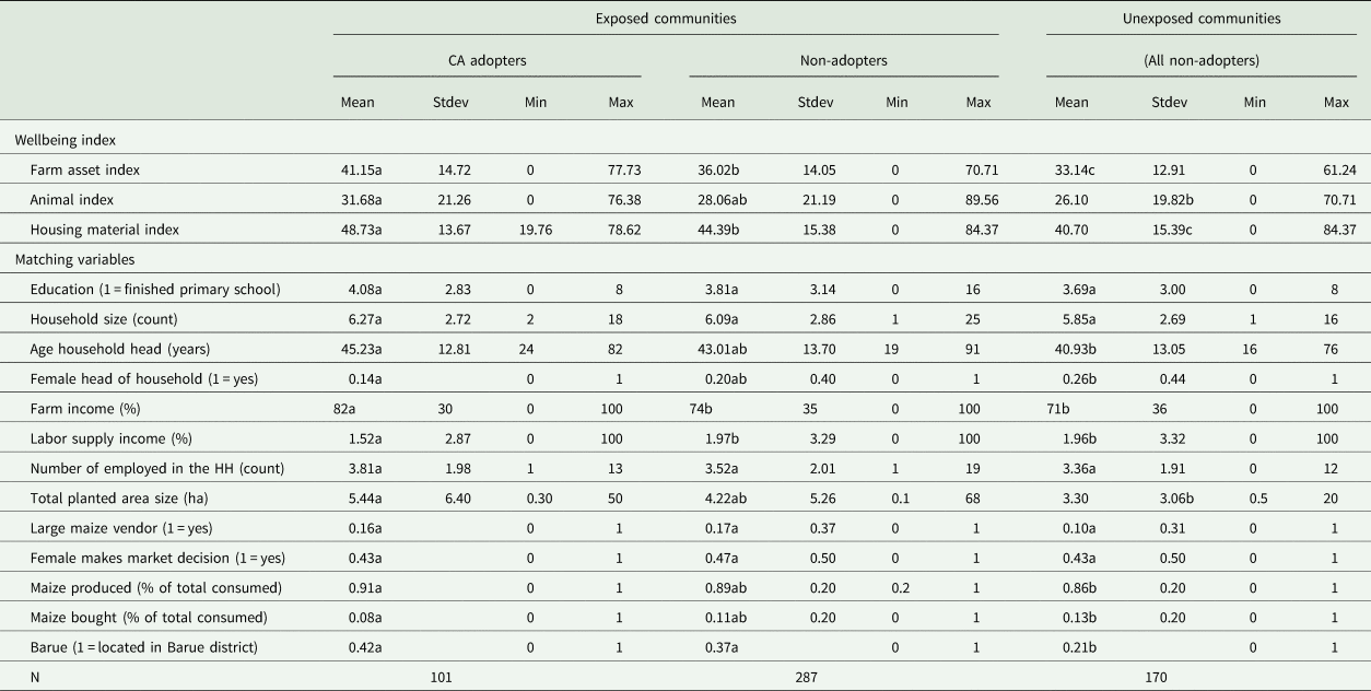
HH, household; Stdev, standard deviation. Row means followed by the same letter not different at the 5% level of significance.
Standard errors of ATT are biased because the variability of the PSM estimator is ignored during the estimation of the ATT's variance (Imbens and Rubin, Reference Imbens and Rubin2015). Lechner (Reference Lechner2002) proposed bootstrapping ATT standard errors to minimize this bias. We used Andrews and Buchinsky's (Reference Andrews and Buchinsky2000) method to determine the optimal number of bootstrap replicates. Andrews and Buchinsky's method is an empirical approach for determining an optimal number of bootstrap replications with the lowest computational cost (Poi, Reference Poi2004). The optimal number of replications was 768. Bootstraps were implemented using Stata 15.1's bootstrap procedure (Stata Corp, 2017).
Rubin (Reference Rubin2001)'s bias reduction (B) and ratio of matched covariates' variances (R) are used to assess PSM performance. A PSM estimator's performance is acceptable when the B statistic is <25% and the R statistic is between 0.5 and two.
Model averaging ATT
A Bayesian hierarchical model was used to generate posterior distributions of the ATT using the estimated differences from matching procedures. The model averaging approach extends Gelman et al. (Reference Gelman, Carlin, Stern, Dunson, Vehtari and Rubin2013)'s meta-analysis methods. The purpose of this procedure is to combine the ATT estimates obtained from the matching procedures, absent consensus on which ATT estimator approximates a true but unobserved ATT into a composite ATT distribution. The ATT from PSM estimators with B statistics <25% and R statistics within their admissible range are included in the model averaging procedure.
Let $\overline {\Delta Y} _{jk}$ indicate an ATT estimate of the j = 1…11 matching procedure for the kth index, with a known standard error σ jk. The first level of the hierarchical model assumes that the ATT are distributed as:

with a corresponding likelihood of $\ell ( \overline {\Delta Y} _{jk}\vert {\rm \theta }_{jk}, \;{\rm \sigma }_{jk})$ and θjk an effect estimate. The effect estimate is a function of an overall average treatment effect on the treated (e.g., CA adopters) for index k, μk, and a precision parameter τk:

with ɛjk a standard normal random variable with E[ɛjk] = 0 and Var[ɛjk] = 1. The prior for the mean parameter is μk ~ Normal(0, 10). The precision parameter's prior is τk ~ Exponential(1). The exponential prior carries no more information than an average standard deviation, which is the inverse of the rate (McElreath, Reference Mcelreath2020).
Posterior distributions of the parameters are recovered using R-Stan's Hamiltonian Monte Carlo No U-turn Sampler (HMC-NUTS) (Hoffman and Gelman, Reference Hoffman and Gelman2014). We ran four chains with a warm-up of 4000 iterations and an additional 4000 iterations to generate posterior distributions for each index's ATT. Chain convergence was verified using Gelman and Rubin's (Reference Gelman and Rubin1992) diagnostic, $\hat{R}$ . Diagnostics approaching one indicate chain convergence. We use the posterior distribution of the average ATT difference between adopters and non-adopters (μk) to compare differences in wellbeing between treatment and counterfactual households.
Results
The farm asset index was significantly higher for CA adopters (41.15) compared with non-adopting households in exposed communities (36.02, difference = 5.13) and households in unexposed villages (33.14, difference from CA adopters = 8.01) (Table 2). Farmers practicing CA reported higher wealth related to farm tool ownership compared to non-adopters in exposed and unexposed communities. For the livestock index, households practicing CA recorded an average of 31.68 points compared to an average of 28.06 and 26.10 for non-adopters in exposed and unexposed villages, respectively (differences from CA adopters, 3.52 and 6.58, respectively). The livestock index for adopters and non-adopters in exposed village was not significantly different. The livestock index for households in unexposed communities was significantly lower than the index average for adopters, but not different when compared to non-adopters in exposed villages (Table 2).
The housing material index was significantly higher for adopters (48.73) compared with non-adopters in exposed villages (Table 2, 44.39, difference = 4.34). This means that adopters used materials that were more durable for home construction. The household material index for unexposed villages (40.70) was significantly lower than the materials index for adopters and non-adopters in exposed villages (difference, 8.03). Although adopters appear to be better off in terms of all wellbeing indices, the univariate comparisons do not control for confounding factors caused by self-selection.
Household and farm characteristics
Education was not significantly different across adopters and non-adopters in both exposed and unexposed communities (Table 2). The average proportion for primary school completion for CA farmers and conventional farmers in exposed communities was 4.1 and 3.8%, respectively. About 3.7% of the households in unexposed villages finished primary school.
Household size was not significantly different across CA and non-adopter households (Table 2). The average for CA households was approximately seven persons per household and a mean of six persons for non-adopters in exposed communities. The mean comparison for the age of the household head was significantly different among the three groups. Household heads practicing CA and non-adopters in exposed villages were aged 45 and 43, respectively. The average household head age for non-adopters in unexposed villages was 41 years.
The proportion of female-headed households was significantly different among CA households and non-adopters in exposed and unexposed villages (Table 2). Females were household heads for 14% of the adopters, and for non-adopters in exposed and unexposed villages, the average was 20 and 26%, respectively.
CA adopters depend more on income from agriculture. Income generated from farm activities was significantly different among CA adopters and non-adopters in exposed villages (Table 2). CA farmers reported that 82% of their income was from farm agricultural sales, while non-adopters in exposed villages reported that sales made up 74% of their household income. The share of income from farm sales was not different between CA non-adopters in exposed villages and households in unexposed villages (71%). There were no differences in income generated from farm sales among CA adopters and households in unexposed communities.
Grabowski et al. (Reference Grabowski, Kerr, Haggblade and Kabwe2016) found a negative relationship between CA adoption and income for Zambian smallholders. In Mozambique, the share of off-farm income for CA adopters (1.5%) was lower compared to non-adopters in exposed communities and households in unexposed villages (Table 2). Wage labor income was not different between CA non-adopters (1.97%) and households in unexposed communities (1.96%). These findings corroborate with those of household income. CA adopters rely more on farming activities for income.
Total land holdings were not significantly different for households in exposed villages, but CA farmers owned significantly more land compared to households in unexposed communities (Table 2). Average land holdings for CA adopters were 5.44 hectares. Non-adopters in exposed communities owned, on average, 4.37 hectares, whereas the average land holding area for households in unexposed communities was 3.31 hectares. Farms in exposed communities were larger than households in unexposed villages were.
Female participation in agricultural markets was at 43% for CA households, 47% for non-adopters in exposed villages, and 43% in unexposed villages (Table 2). These means are not significantly different. CA adopters consumed relatively more of the maize they produced (91%) compared to households in unexposed communities (86%, Table 2). Consumption of maize by non-adopters in exposed communities (89%) was not different from CA adopters or households in unexposed communities.
CA adoption and ATT
For the exposed village comparison, Rubin (Reference Rubin2001)'s diagnostics indicate that the caliper NN method with five neighbors and replacement, both kernel PSM, the Mahalanobis 1-to-1 match with replacement, and the AIPW estimators performed well in terms of re-balancing the covariates used to match households (Table 3, acceptable methods denoted by ‘#’). The caliper NN method with one neighbor without replacement, the Gaussian kernel PSM, and the AIPW estimators performed adequately for the comparison of CA adopters with households in unexposed villages (Table 3). For all PSM, the matched sample size was 333. We only discuss the ATT with bias reduction statistics less than 25% and variance ratios between [0.5, 2].
Rubin's (Reference Rubin2001) bias reduction and variance similarity statisticsa

a Rubin's (Reference Rubin2001) diagnostics are B (average bias reduction) and R (ratio of variances) for matching covariates. Balance problems are present when B exceeds 25 and R is outside the [0.5, 2] range. * indicates concerning matches.
The livestock index ATT for CA adopters in exposed villages was not significantly different for any PSM estimator (Table 4). Nor was the livestock index ATT different from zero for the comparison of CA adopters with households in unexposed communities (Table 5). This is an unsurprising result. Most households in the region practice row crop and vegetable production. In Mozambique, CA adoption is relatively low in areas where livestock production is the dominant agricultural activity because farmers retain residues for animal feedstock (Thierfelder et al., Reference Thierfelder, Cheesman and Rusinamhodzi2013). Maintaining field residue is an important component of CA, but it is a challenge to implement in communities that rely on livestock for income and nutrition (Silici et al., Reference Silici, Bias and Cavane2015).
Average treatment effects comparing conservation agriculture adopters and non-adopters in exposed communities

***, **, * denote 1, 5 and 10% respectively. N = 333 matched cases.
#, pass Rubin's (Reference Rubin2001) diagnostics for bias reduction and variance similarity (see Table 3).
a C = 1 are conservation agriculture adoption (non-adopters, otherwise).
b Bootstrapped standard errors are in parentheses. Number of bootstrap replications is 768 (Andrews and Buchinsky, Reference Andrews and Buchinsky2000).
c Caliper is 0.25 standard deviations.
Average treatment effects comparing conservation agriculture adopter households with unexposed households

***, **, * denote 1, 5 and 10% respectively. N = 244 matched cases.
#, pass Rubin's (Reference Rubin2001) diagnostics for bias reduction and variance similarity (see Table 3).
a C = 1 are conservation agriculture adoption (non-adopters, otherwise).
b Bootstrapped standard errors are in parentheses. Number of bootstrap replications is 768 (Andrews and Buchinsky, Reference Andrews and Buchinsky2000).
c Caliper is 0.25 standard deviations.
The evidence is mixed for substantiating differences between the farm asset and house materials ATT and CA adoption. The farm asset index ATT for adopters in exposed villages was always higher than the same index for the counterfactual group of non-adopting households. The Epanechnikov kernel ATT (ATT ± standard error, 2.91 ± 1.48), the Mahalanobis 1-to-1 estimator with replacement (ATT, 3.82 ± 1.78) and the AIPW estimator (3.29 ± 1.29) indicate that ownership of farm tools and the quality of material used to construct houses was significantly higher for CA adopters (Table 4). However, the ATT was not different from zero for the caliper NN(5) with replacement or the Gaussian kernel PSM. The ATT differences are lower than the univariate comparison, suggesting that univariate differences in the wellbeing indices are biased upward. Two of the three admissible matching estimators indicated significant differences between the farm asset index ATT for CA adopters and the counterfactual group of households in unexposed villages. For this comparison, ATT ranged between 2.57 and 4.19 (Table 5).
The results were similar for the housing material index (Table 4). In this case, significant differences between CA adopters and the counterfactual group in exposed villages were observed under the Gaussian kernel estimator (ATT, 3.42 ± 1.86), the 1-to-1 Mahalanobis estimator (ATT, 4.64 ± 2.49) and the AIPW estimator (4.36 ± 1.67). The housing material index was unambiguously higher for CA-adopting households compared to the counterfactual case, with significant differences ranging between 7.27 and 7.66 among the three admissible matching estimators (Table 5).
The findings are consistent with previous research. Ng'ombe et al. (Reference Ng'ombe, Kalinda and Tembo2017) used a POM to compare profits from maize production by Zambian smallholders who adopted some or all CA components. They found that income was higher for households that practiced a suite of CA technologies compared with households that adopted piecemeal CA technologies. In their study of CA adoption, Abdulai and Abdul-Rahaman (Reference Abdulai and Abdul-Rahaman2019) also concluded that CA reduced the poverty levels of smallholder farmers in Zambia.
Model-averaged ATT
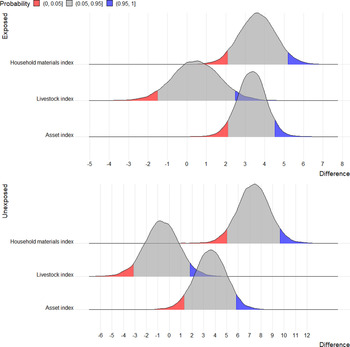
The ATT and their respective standard errors from acceptable PSM estimators (Tables 4 and 5) were used in the model averaging procedure to generate posterior ATT. Gelman and Rubin's $\hat{R}$ diagnostics indicated chain convergence. ATT with lower standard errors exert greater influence over the mean of the treatment effect estimates and the tails of the distribution. The posterior mean ± the estimated standard error for the farm asset index ATT of CA adopters in exposed villages was 3.32 ± 0.53. The lower 5th-percentile of the posterior distribution exceeds zero, suggesting that CA adopters owned relatively more farm assets compared to their non-adopting neighbors in exposed communities (Fig. 1). Similarly, the model-averaged ATT of the housing material index for CA adopters in exposed communities was positive, with a lower 5th-percentile bound exceeding zero (3.63 ± 0.62). The model-averaged ATT for the livestock index of adopters in exposed communities was not different from zero (0.48 ± 0.72). We conclude that CA adopter wellbeing in exposed communities, as measured by the housing material and farm asset index proxy, was, ceteris paribus, higher than it would have been in the counterfactual case of non-adoption.
Posterior distributions of wellbeing index average treatment effects on the treated (ATT). Notes: ‘Difference’ is the ATT for the index values. ‘Exposed’ includes adopting and non-adopting households in communities that had received CA extension. ‘Unexposed’ compares CA adopters in exposed villages (‘treatment’) with households in villages that had not received CA extension (‘control’). Gray shaded areas include 90% of the ATT's posterior distribution.

Model-averaged ATT for the farm asset and housing material indices of CA adopters and households in unexposed communities were positive and significantly different from zero, as evidenced by the lower 5th-percentiles of their respective posterior distributions (Fig. 1). The model-averaged ATT between these groups' farm assets index was 3.58 ± 0.75. For the housing material index, the ATT point estimate for CA adopters and the counterfactual group of households in unexposed villages was 7.34 ± 0.77. There was no difference between the respective groups' livestock ownership indices (−0.66 ± 0.79). We conclude that CA adopters' wellbeing in exposed communities, as measured by the housing material and farm asset indices, was, ceteris paribus, higher than for the counterfactual group composed of households in unexposed communities.
Some general remarks follow. First, the difference between the livestock index for CA adopters and non-adopters is not significant for any comparison. This result is unsurprising. The primary income-generating activity in the region is from row crop production. Secondly, the observed differences in the farm asset indices for CA adopters and non-adopters in both exposed and unexposed communities are similar in magnitude and dispersion (Tables 4 and 5). These commonalities in the farm asset and livestock ownership index ATT are also evident in the model-averaged distributions (Fig. 1). The similarities in ATT differences for these two indices, along with the PSM diagnostics (Table 3), provide some assurance that community-specific attributes, including distance to urban markets, frequency of contact with extension or other community-specific factors omitted from the PSM procedure, are unlikely drivers of the observed differences in the farm asset and livestock ownership indices.
The relative magnitude of the ATT difference for the housing material index between exposed, CA-adopting households and the counterfactual group of unexposed households is quite large compared with the ATT difference in this index for households in exposed communities. While the Rubin diagnostics used to select well-performing PSM suggest that confounding effects are minimized (Appendix Table 3), there are a variety of reasons why this might be the case. One explanation could be that households in unexposed communities may be more vulnerable to poverty and food insecurity. Access to health care, credit, agricultural inputs and other factors may also be affecting the magnitude of the housing material index for this specific comparison. The survey did not collect information on additional variables that could be used to discern why the magnitude is relatively large, and the effect of these unobserved variables on the ATT cannot be discerned. Alternatively, one could argue that the comparison of CA-adopting households in exposed communities with households in unexposed communities is a false equivalence. Exposed communities are those that had already been in contact with agents promoting CA since 2008. However, to the extent that, in the development of a counterfactual scenario, the PSM procedures match, as closely as possible, CA-adopting households in exposed villages to households in the unexposed communities by conditioning on a set of common attributes, then concern over false equivalence is moderated. If there are other unobserved factors omitted from the PSM selection equation (Equation 5), then the exposed–unexposed comparison of the housing material index could be biased. These issues are important caveats for this comparison.
Conclusions
The objective of this study was to determine the impact of CA on smallholder wellbeing in Mozambique. Households that practiced CA were better off in terms of farm assets ownership and the quality of materials used to construct homes. Livestock ownership indices were not different between CA adopters and non-adopters. Smallholder households who used CA had, ceteris paribus, higher wellbeing indices compared to counterfactual households that did not practice CA. The effect magnitude was lower for the counterfactual group developed in exposed communities compared to the counterfactual group represented by households in unexposed communities.
The findings are relevant for understanding the potential effects of CA adoption on smallholder household wellbeing. In the long term, adopting yield-enhancing practices like CA can result in farmers accumulating wealth. The findings are consistent with other research that used similar POM methodologies to gauge the effect of CA adoption on household status for smallholders in neighboring Zambia.
A limitation of this study is the cross-sectional nature of the survey. Ideally, a before-after comparison of the wellbeing indicators is desirable for conducting a matched difference-in-difference comparison of wellbeing status. An even more powerful, unambiguous result would be achievable if CA could be randomly assigned among households. However, building this type of panel data is expensive, risky and difficult to implement in most remote farming regions of Mozambique.
Supplementary material
The supplementary material for this article can be found at https://doi.org/10.1017/S1742170521000430.
Acknowledgements
Research was supported by the United States Agency for International Development’s Sustainable Agriculture and Natural Resource Management/ Collaborative Research Support Program and the Sparks Chair in Agricultural Sciences & Natural Resources and the Oklahoma Agricultural Experiment Station, Stillwater, OK, USA. The authors declare no competing interests.