2.1 Governing equations

Figure 1.

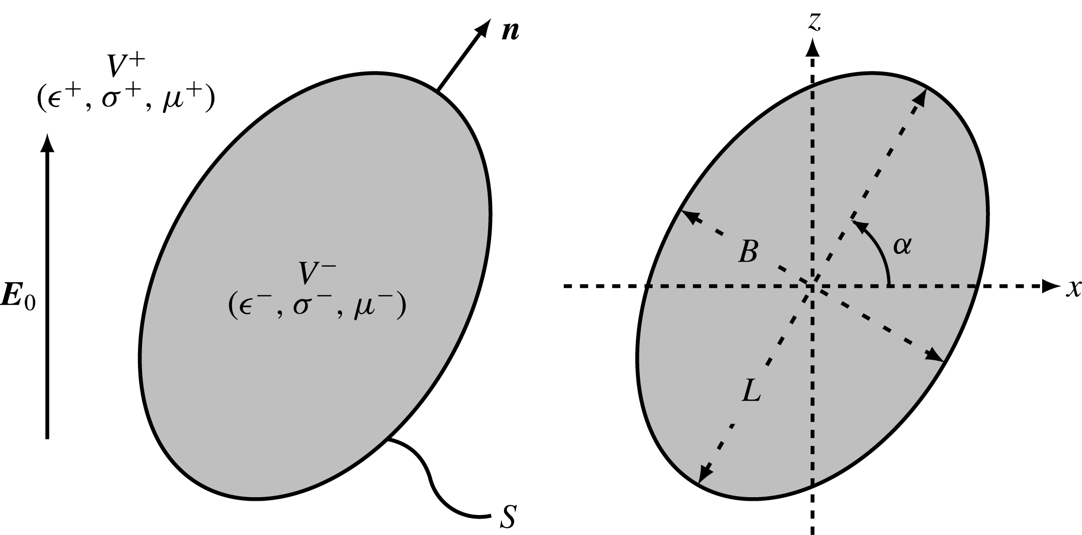
Problem definition: a liquid droplet with surface $S$ and outward unit normal $\boldsymbol{n}$ is suspended in an unbounded domain and placed in a uniform electric field $\boldsymbol{E}_{0}$ pointing in the vertical direction. $V^{\pm }$ denote the exterior and interior domains, respectively, and $(\unicode[STIX]{x1D716}^{\pm },\unicode[STIX]{x1D70E}^{\pm },\unicode[STIX]{x1D707}^{\pm })$ are the corresponding dielectric permittivities, electric conductivities and dynamic viscosities. The drop’s major and minor axis lengths are denoted by $L$ and $B$ , and the major axis is tilted at an angle $\unicode[STIX]{x1D6FC}$ with respect to the horizontal direction.

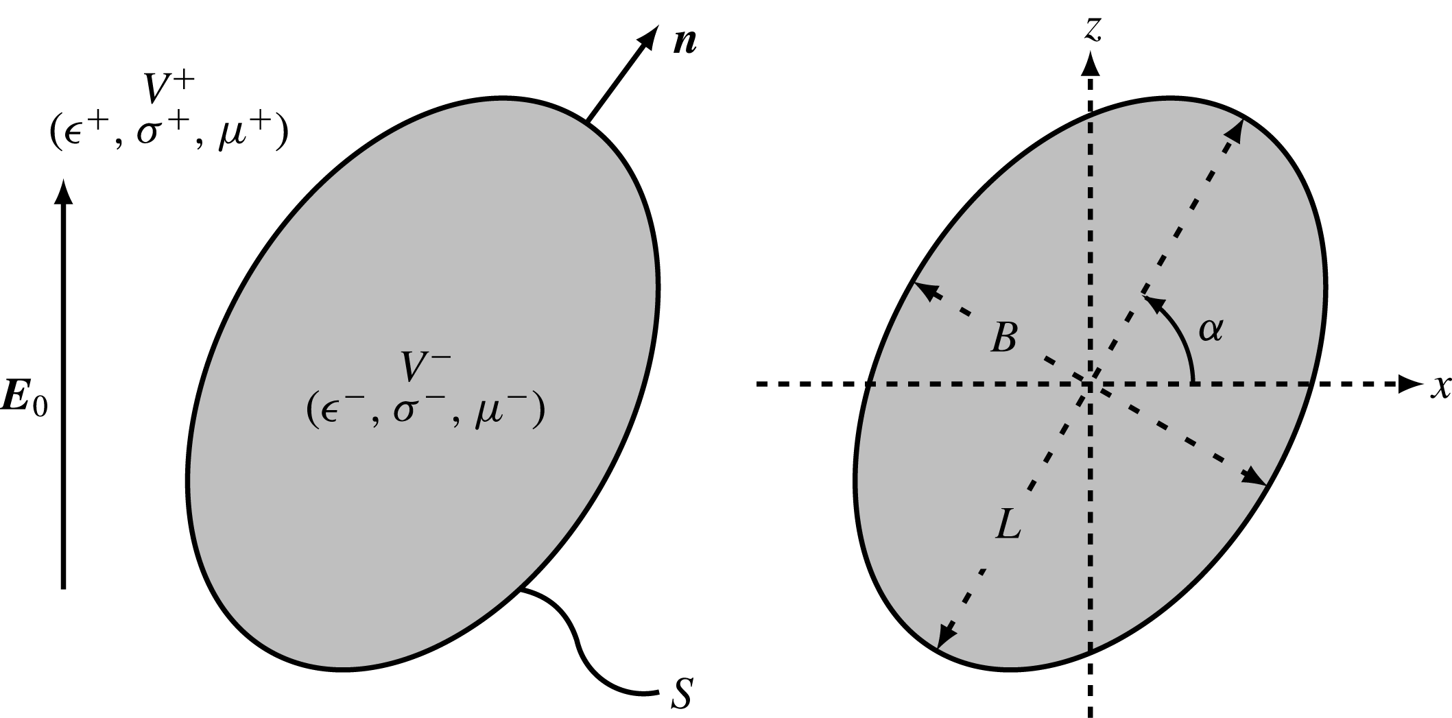
We consider an uncharged neutrally buoyant liquid droplet with undeformed radius $a$ occupying volume $V^{-}$ in an infinite fluid medium $V^{+}$ and subject to a uniform electric field $\boldsymbol{E}_{0}=E_{0}\hat{\boldsymbol{z}}$ as depicted in figure 1. The drop surface is denoted as $S$ and has an outward unit normal $\boldsymbol{n}$ . Let $(\unicode[STIX]{x1D716}^{\pm },\unicode[STIX]{x1D70E}^{\pm },\unicode[STIX]{x1D707}^{\pm })$ be the dielectric permittivities, electric conductivities and dynamic viscosities of the exterior and interior fluids, respectively. In the Melcher–Taylor leaky dielectric model (Melcher & Taylor Reference Melcher and Taylor1969), all charges in the system are concentrated on the drop surface, so that the electric potential in both fluid domains is harmonic:

On the drop surface, the electric potential is continuous, as is the tangential component of the local electric field:

where $\boldsymbol{E}_{t}^{\pm }=(\unicode[STIX]{x1D644}-\boldsymbol{n}\boldsymbol{n})\boldsymbol{\cdot }\boldsymbol{E}^{\pm }$ and $\boldsymbol{E}^{\pm }=-\unicode[STIX]{x1D735}\unicode[STIX]{x1D711}^{\pm }$ . We have introduced the notation $\unicode[STIX]{x27E6}\,f(\boldsymbol{x})\unicode[STIX]{x27E7}\equiv f^{+}(\boldsymbol{x})-f^{-}(\boldsymbol{x})$ for any field variable $f(\boldsymbol{x})$ defined on both sides of the interface. Unlike $\boldsymbol{E}_{t}$ , the normal component of the electric field $E_{n}^{\pm }=\boldsymbol{n}\boldsymbol{\cdot }\boldsymbol{E}^{\pm }$ undergoes a jump due to the mismatch in electrical properties between the two media (Landau, Lifshitz & Pitaevskiì Reference Landau, Lifshitz and Pitaevskiì1984), which results in a surface charge distribution $q(\boldsymbol{x})$ related to the normal displacement field by Gauss’s law:

The surface charge density $q$ evolves due to two distinct mechanisms: ohmic currents from the bulk and advection by the fluid flow with velocity $\boldsymbol{v}(\boldsymbol{x})$ on the drop surface. Accordingly, it satisfies the conservation equation:

where $\unicode[STIX]{x1D735}_{s}\equiv (\unicode[STIX]{x1D644}-\boldsymbol{n}\boldsymbol{n})\boldsymbol{\cdot }\unicode[STIX]{x1D735}$ is the surface gradient operator. On neglecting unsteady terms and surface charge convection, equation (2.4) reduces to the simpler boundary condition $\unicode[STIX]{x27E6}\unicode[STIX]{x1D70E}E_{n}\unicode[STIX]{x27E7}=0$ used in a number of previous studies (Sherwood Reference Sherwood1988; Baygents et al. Reference Baygents, Rivette and Stone1998; Lac & Homsy Reference Lac and Homsy2007).

The fluid velocity field $\boldsymbol{v}^{\pm }(\boldsymbol{x})$ and corresponding pressure field $p^{\pm }(\boldsymbol{x})$ satisfy the Stokes equations in both fluid domains:

The velocity is continuous on the drop surface:

and, in the absence of Marangoni effects, the jumps in electric and hydrodynamic tractions across the interface balance interfacial tension forces:

Here, $\unicode[STIX]{x1D6FE}$ is the constant surface tension and $\unicode[STIX]{x1D735}_{s}\boldsymbol{\cdot }\boldsymbol{n}=2\unicode[STIX]{x1D705}_{m}$ is twice the mean surface curvature. The jumps in tractions are expressed in terms of the Maxwell stress tensor $\unicode[STIX]{x1D64F}^{E}$ and hydrodynamic stress tensor $\unicode[STIX]{x1D64F}^{H}$ as

The jump in electric tractions can also be expressed as

The first term on the right-hand side captures the tangential electric force on the interface arising from the action of the tangential field on the interfacial charge distribution. The second term captures normal electric stresses and can be interpreted as the jump in an electric pressure $p^{E}=(\unicode[STIX]{x1D716}(E_{n}^{2}-E_{t}^{2}))/2$ (Lac & Homsy Reference Lac and Homsy2007).

2.2 Non-dimensionalization

Non-dimensionalization of the governing equations yields five dimensionless groups, three of which are ratios of material properties typically defined as:

The low-drop-viscosity limit $\unicode[STIX]{x1D706}\rightarrow 0$ describes a bubble, whereas $\unicode[STIX]{x1D706}\rightarrow \infty$ describes a rigid particle. The product $RQ$ can also be interpreted as the ratio of the inner to outer charge relaxation times:

A possible choice for the two remaining dimensionless numbers consists of the electric capillary number $Ca_{E}$ , denoting the ratio of electric to capillary forces, and electric Mason number $Ma$ , denoting the ratio of viscous to electric stresses:

Here, $\unicode[STIX]{x1D70F}_{MW}$ is the Maxwell–Wagner relaxation time, or characteristic time scale for polarization of the drop surface upon application of the field (Das & Saintillan Reference Das and Saintillan2013):

$Ma$ is also directly related to the ratio of the electric field magnitude $E_{0}$ to the critical electric field $E_{c}$ for onset of Quincke rotation of a rigid sphere as

where

For a rigid sphere, Quincke rotation occurs when $E_{0}>E_{c}$ , or $Ma<(\overline{\unicode[STIX]{x1D716}}-\overline{\unicode[STIX]{x1D70E}})/2$ , thus necessitating the application of a strong electric field. For the critical electric $E_{c}$ to take on a real value, the condition $\overline{\unicode[STIX]{x1D716}}>\overline{\unicode[STIX]{x1D70E}}$ , which is equivalent to $RQ>1$ or $\unicode[STIX]{x1D70F}^{+}>\unicode[STIX]{x1D70F}^{-}$ , needs to be satisfied; this generally implies that the drop is less conducting than the suspending fluid. It is useful to note the direct correspondence between $Ma$ and the electric Reynolds number $Re_{E}^{+}$ defined by other authors (Salipante & Vlahovska Reference Salipante and Vlahovska2010; Lanauze et al. Reference Lanauze, Walker and Khair2015; Schnitzer & Yariv Reference Schnitzer and Yariv2015):

Finally, an additional dimensionless group can also be constructed by taking the ratio of the capillary time $\unicode[STIX]{x1D70F}_{\unicode[STIX]{x1D6FE}}=\unicode[STIX]{x1D707}^{+}(1+\unicode[STIX]{x1D706})a/\unicode[STIX]{x1D6FE}$ and Maxwell–Wagner relaxation time $\unicode[STIX]{x1D70F}_{MW}$ and is independent of field strength (Salipante & Vlahovska Reference Salipante and Vlahovska2010):

For a fixed set of material properties, varying $Ca_{MW}$ is equivalent to varying drop size $a$ . In the remainder of the paper, we exclusively use dimensionless variables by scaling lengths with $a$ , electric fields with $E_{0}$ and times with $\unicode[STIX]{x1D70F}_{MW}$ . In addition to $R$ , $Q$ and $\unicode[STIX]{x1D706}$ , we primarily use $Ca_{E}$ and $Ma$ as dimensionless groups, though some of the results in § 4 will also be shown in terms of $E_{0}/E_{c}$ and $Ca_{MW}$ .

3.1 Electric problem

The solution of Laplace’s equation (2.1) is best formulated using boundary integral equations (Jaswon Reference Jaswon1963; Symm Reference Symm1963; Pozrikidis Reference Pozrikidis2002). Following previous studies in the field (Sherwood Reference Sherwood1988; Baygents et al. Reference Baygents, Rivette and Stone1998; Lac & Homsy Reference Lac and Homsy2007; Lanauze et al. Reference Lanauze, Walker and Khair2015) we represent the potential in terms of the single-layer density $\unicode[STIX]{x27E6}E_{n}(\boldsymbol{x})\unicode[STIX]{x27E7}$ as

Here, $\boldsymbol{x}_{0}$ is the evaluation point for the potential and can be anywhere in space, whereas $\boldsymbol{x}$ denotes the integration point which is located on the drop surface. The Green’s function or fundamental solution of Laplace’s equation in an unbounded domain is given by

Note that (3.1) is valid in both fluid phases as well as on the interface since the Green’s function is continuous across $S$ . The equation is weakly singular, however, when $\boldsymbol{x}=\boldsymbol{x}_{0}$ , though the singularity can be removed analytically by introducing plane polar coordinates in the parametric plane defining the local surface (Pozrikidis Reference Pozrikidis2002). Knowledge of the single-layer potential density $\unicode[STIX]{x27E6}E_{n}(\boldsymbol{x})\unicode[STIX]{x27E7}$ on the interface therefore allows one to determine the electric potential anywhere in space by simple integration, which prompts us to seek an equation for $\unicode[STIX]{x27E6}E_{n}(\boldsymbol{x})\unicode[STIX]{x27E7}$ in terms of the surface charge density $q$ . We first take the gradient of (3.1) to obtain an integral equation for the electric field in the fluid:

The derivative of the Green’s function undergoes a discontinuity at the interface, which needs to be accounted for when the evaluation point is on the boundary (Pozrikidis Reference Pozrikidis2011):

The integral equation for the electric field is strongly singular. However, taking a dot product on both sides with the unit normal $\boldsymbol{n}(\boldsymbol{x}_{0})$ reduces the singularity by one order. Averaging the normal components of the field outside and inside the drop then yields

where the weak singularity can now be removed analytically following Sellier (Reference Sellier2006) by subtracting $\unicode[STIX]{x27E6}E_{n}(\boldsymbol{x}_{0})\unicode[STIX]{x27E7}$ from the single-layer density:

The scalar function $L(\boldsymbol{x}_{0})$ is a purely geometrical quantity depending on drop shape and expressed as (Sellier Reference Sellier2006)

Gauss’s law also allows us to express $E_{n}^{+}$ and $E_{n}^{-}$ on each side of the interface in terms of the jump in normal electric field,

which, after substitution into (3.6), provides a regular integral equation for the jump $\unicode[STIX]{x27E6}E_{n}\unicode[STIX]{x27E7}$ :

The jump $\unicode[STIX]{x27E6}E_{n}\unicode[STIX]{x27E7}$ can therefore be computed from (3.9) for a given surface charge density after discretization of the integral on a mesh, yielding a large linear system that is solved iteratively. Further details of the numerical implementation are given in § 3.3 and in appendix A. Having obtained $\unicode[STIX]{x27E6}E_{n}\unicode[STIX]{x27E7}$ , the normal components $E_{n}^{+}$ and $E_{n}^{-}$ are easily obtained using (3.8).

The tangential component of the electric field can then be evaluated using (3.4); however, care must be taken to remove the strong singularity in the kernel. Here, we adopt instead an indirect method in which we first compute the electric potential $\unicode[STIX]{x1D711}$ using (3.1) then differentiate it numerically on the drop surface to obtain $\boldsymbol{E}_{t}$ . Once the normal and tangential components of the electric field are known, we can determine the jump in the normal component of ohmic currents $\unicode[STIX]{x27E6}\unicode[STIX]{x1D70E}E_{n}\unicode[STIX]{x27E7}$ as well as the jump in electric tractions $\unicode[STIX]{x27E6}\,\boldsymbol{f}^{E}\unicode[STIX]{x27E7}$ using (2.10).

3.2 Flow problem

The applied electric field induces fluid motion inside and outside the drop. The need to solve for the fluid flow is twofold, as it affects the surface charge distribution according to (2.4) and causes deformations of the interface, which is a material surface advected by the flow. The flow problem is solved after application of the dynamic boundary condition (2.7) to obtain the hydrodynamic traction jump $\unicode[STIX]{x27E6}\,\boldsymbol{f}^{H}\unicode[STIX]{x27E7}$ on the drop–fluid interface. Assuming creeping flow, we use the Stokes boundary integral equation to represent the fluid velocity as (Rallison & Acrivos Reference Rallison and Acrivos1978; Pozrikidis Reference Pozrikidis2002)

where $\unicode[STIX]{x1D705}=(1-\unicode[STIX]{x1D706})/(1+\unicode[STIX]{x1D706})$ and $\unicode[STIX]{x1D642}(\boldsymbol{x}_{0};\boldsymbol{x})$ and $\unicode[STIX]{x1D64F}(\boldsymbol{x}_{0};\boldsymbol{x})$ denote the free-space Green’s functions for the Stokeslet and stresslet, respectively:

The usual negative sign in the definition of the stresslet appears if $\boldsymbol{r}$ is defined as $\boldsymbol{x}-\boldsymbol{x}_{0}$ . Note that $\unicode[STIX]{x1D705}=\pm 1$ corresponds to the case of a bubble ( $\unicode[STIX]{x1D706}\rightarrow 0$ ) and solid particle ( $\unicode[STIX]{x1D706}\rightarrow \infty$ ), respectively. The interfacial velocity appearing in the double-layer potential is yet unknown, but an integral equation for $\boldsymbol{v}$ on the surface can be obtained by moving the evaluation point $\boldsymbol{x}_{0}$ to the boundary $S$ . In dimensionless form, it reads:

The forcing term in this equation is contained in the hydrodynamic traction jump $\unicode[STIX]{x27E6}\,\boldsymbol{f}^{H}\unicode[STIX]{x27E7}$ . After discretization of the integral, equation (3.12) yields a dense linear system that is again solved iteratively. The weak singularity appearing in the double-layer potential in the original equation (3.10) has been removed by using appropriate integral identities; the weak singularity of the single-layer potential, on the other hand, disappears after introducing plane polar coordinates (Pozrikidis Reference Pozrikidis1992). It is well known that the integral equation (3.12) admits arbitrary rigid body motions and uniform expansion as eigensolutions, resulting in the ill conditioning of the linear system for $\unicode[STIX]{x1D706}\gg 1$ or $\unicode[STIX]{x1D706}\ll 1$ and leading to poor convergence of the solution (Zinchenko, Rother & Davis Reference Zinchenko, Rother and Davis1997). We employ Wielandt’s deflation technique to eliminate $\unicode[STIX]{x1D705}=\pm 1$ from the spectrum of the integral equation to cure the ill conditioning (Kim & Karrila Reference Kim and Karrila2013); see appendix B for details. Once the interfacial velocity is known, the nodes are advected with the normal component of the fluid velocity; the heuristic mesh relaxation algorithm of Loewenberg & Hinch (Reference Loewenberg and Hinch1996) is applied in the tangential direction so as to reduce mesh distortion.

3.3 Summary of the numerical method

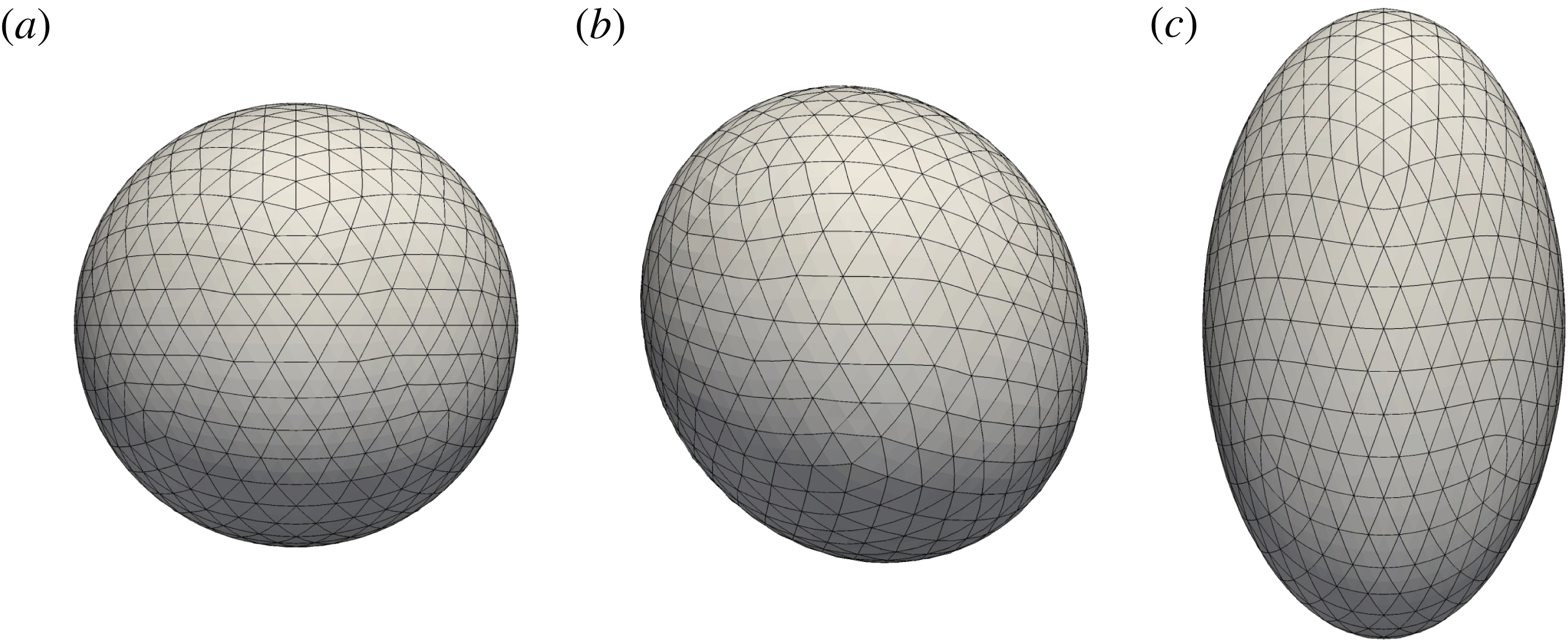
We solve integral equations (3.1), (3.9) and (3.12) numerically using the boundary element method on a discrete representation of the drop surface (Pozrikidis Reference Pozrikidis2002). The initially spherical surface is first discretized by successive subdivision of an icosahedron, by which each triangular element is subdivided into four new triangles whose nodes are projected onto the sphere (Loewenberg & Hinch Reference Loewenberg and Hinch1996). This leads to a highly uniform triangular mesh, in which we treat each element as a six-node curved element, thus allowing for computation of the local curvature. The results in the Taylor regime presented below were obtained on a surface with $N_{\triangle }=1280$ elements and 2562 nodes, corresponding to $N_{d}=3$ subdivisions; most simulations in the Quincke regime, where deformations are weaker, used a mesh of $N_{\triangle }=320$ elements and 642 nodes obtained after $N_{d}=2$ successive subdivisions. Typical meshes with $N_{d}=3$ are shown in figure 2 for different levels of deformation, and convergence results in the Taylor regime will be presented in figure 3. The evaluation of integrals and the calculation of geometrical properties such as the unit normal and curvature on the discretized surface are standard and are outlined in appendix A.

Figure 2.

Discretized mesh: $N_{\triangle }=1280$ six-node curved elements. (a) An initially spherical mesh at time $t=0$ , (b) a deformed mesh for a tilted drop in the Quincke regime corresponding to the case of figure 6 and (c) a deformed mesh of a prolate drop in the Taylor regime (system 3), where we applied the mesh relaxation algorithm of Loewenberg & Hinch (Reference Loewenberg and Hinch1996).

Figure 3.

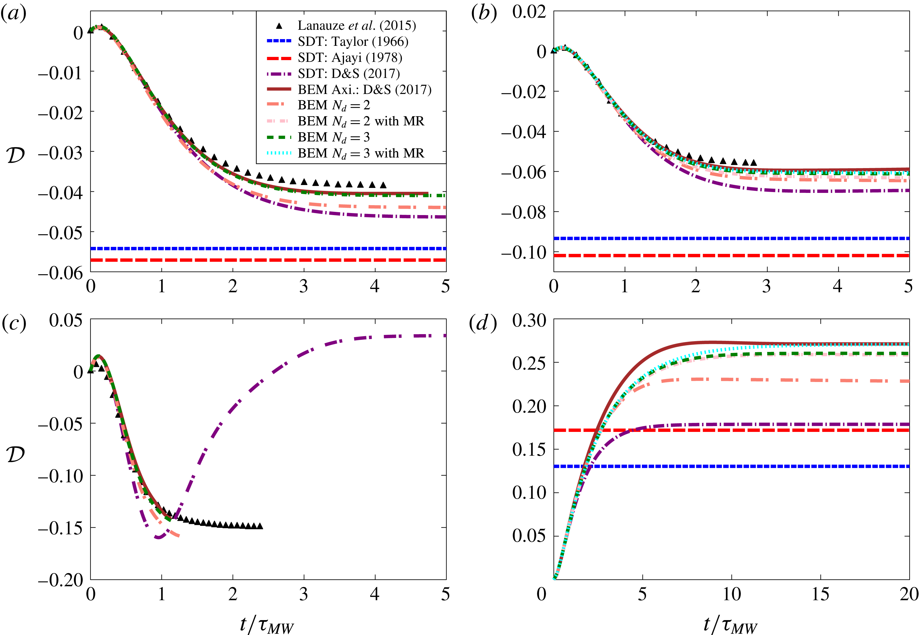
Deformation parameter ${\mathcal{D}}$ as a function of time for the parameters of: (a) system 1a, (b) system 1b, (c) system 1c and (d) system 3. Boundary element (BEM) results are compared to the experiments of Lanauze et al. (Reference Lanauze, Walker and Khair2015) in the case of oblate drops, and to various small-deformation theories (SDT). The steady deformation values predicted by the models of Taylor (Reference Taylor1966) and Ajayi (Reference Ajayi1978) in the case of system 1c are $-0.75$ and $-1.40$ , respectively, and out of the frame of the figure. The effect of the mesh relaxation (MR) algorithm is also shown and found to be greater when large deformations arise (system 3).

The numerical algorithm during one integration step can be summarized as follows:

1. (i) Given an interfacial charge distribution $q$ (which is taken to be uniformly zero at $t=0$ ), solve for $\unicode[STIX]{x27E6}E_{n}\unicode[STIX]{x27E7}$ , $E_{n}^{+}$ and $E_{n}^{-}$ by inverting equation (3.9) numerically, together with (3.8). Discretization of the integrals in (3.9) yields a large algebraic system which we solve iteratively using GMRES (Saad & Schultz Reference Saad and Schultz1986).

2. (ii) Evaluate the electric potential $\unicode[STIX]{x1D711}$ on the drop surface using (3.1), where the single-layer density $\unicode[STIX]{x27E6}E_{n}\unicode[STIX]{x27E7}$ is known.

3. (iii) Differentiate $\unicode[STIX]{x1D711}$ on the drop surface using the method outlined in appendix A to obtain the tangential component $\boldsymbol{E}_{t}=-(\unicode[STIX]{x1D644}-\boldsymbol{n}\boldsymbol{n})\boldsymbol{\cdot }\unicode[STIX]{x1D735}\unicode[STIX]{x1D711}$ of the electric field.

4. (iv) Calculate the jump in hydrodynamic tractions $\unicode[STIX]{x27E6}\,\boldsymbol{f}^{H}\unicode[STIX]{x27E7}$ using the dynamic boundary condition (2.7), where electric tractions and surface tension forces are known from the solution of the electric problem and from the current geometry.

5. (v) Solve for the interfacial velocity $\boldsymbol{v}$ by inverting the boundary integral equation (3.12), which again yields an algebraic system after discretization of the integrals.

6. (vi) Update the surface charge density $q$ and advance the position of the surface nodes $\boldsymbol{x}_{i}$ by numerical integration of the charge conservation equation and kinematic boundary condition,

   (3.13) $$\begin{eqnarray}\displaystyle & \displaystyle \frac{\unicode[STIX]{x2202}q}{\unicode[STIX]{x2202}t}=\frac{Q+2}{1+2R}(E_{n}^{-}-RE_{n}^{+})-\unicode[STIX]{x1D735}_{s}\boldsymbol{\cdot }(q\boldsymbol{v}_{t})+\boldsymbol{v}_{m}\boldsymbol{\cdot }\unicode[STIX]{x1D735}_{s}q, & \displaystyle\end{eqnarray}$$
   (3.14) $$\begin{eqnarray}\displaystyle & \displaystyle \frac{\text{d}\boldsymbol{x}_{i}}{\text{d}t}=\boldsymbol{v}_{n}(\boldsymbol{x}_{i})+\boldsymbol{v}_{m}(\boldsymbol{x}_{i}), & \displaystyle\end{eqnarray}$$
   where $\boldsymbol{v}_{t}=(\unicode[STIX]{x1D644}-\boldsymbol{n}\boldsymbol{n})\boldsymbol{\cdot }\boldsymbol{v}$ and $\boldsymbol{v}_{n}=(\boldsymbol{v}\boldsymbol{\cdot }\boldsymbol{n})\boldsymbol{n}$ are the tangential and normal components of the fluid velocity on the interface and $\boldsymbol{v}_{m}$ is an artificial mesh relaxation velocity. Charge is defined at the position of the moving surface nodes, which are evolved with the normal velocity $\boldsymbol{v}_{n}$ only so as to reduce mesh distortion; transport of charge by the tangential fluid velocity is instead captured by the advective term $-\unicode[STIX]{x1D735}_{s}\boldsymbol{\cdot }(q\boldsymbol{v}_{t})$ in the charge transport equation. To further limit mesh distortion, we use an artificial tangential mesh relaxation velocity $\boldsymbol{v}_{m}$ in (3.14), which is determined using the method of Loewenberg & Hinch (Reference Loewenberg and Hinch1996); the last advective term with velocity $-\boldsymbol{v}_{m}$ in (3.13) is added to prevent mesh relaxation from affecting charge transport. In the results shown below, mesh relaxation was used in the Taylor regime to capture large drop deformations; it was abandoned in the Quincke regime where it was found to cause numerical instabilities. Numerical integration of (3.13)–(3.14) is performed explicitly in time using a second-order Runge–Kutta scheme.

The charge conservation equation (3.13) requires numerical evaluation of the surface divergence and gradient appearing on the right-hand side. These quantities are obtained by analytical differentiation based on the parametrization discussed in appendix A; an alternate method based on finite volumes (Yon & Pozrikidis Reference Yon and Pozrikidis1998) and a semi-implicit scheme wherein the linear $\unicode[STIX]{x27E6}\unicode[STIX]{x1D70E}E_{n}\unicode[STIX]{x27E7}$ and nonlinear $\unicode[STIX]{x1D735}_{s}\boldsymbol{\cdot }(q\boldsymbol{v}_{t})$ terms are treated implicitly and explicitly, respectively, were also attempted but did not produce significant differences in the results. The numerical method was tested extensively by first considering the case of a solid spherical particle under Quincke rotation, for which an exact analytical solution based on spherical harmonics is available (Das & Saintillan Reference Das and Saintillan2013), and by comparison with previous numerical studies of drop dynamics in simple shear flow (Kennedy, Pozrikidis & Skalak Reference Kennedy, Pozrikidis and Skalak1994) and under electric fields in the absence of charge convection (Lac & Homsy Reference Lac and Homsy2007).

4.1 Taylor regime

Table 1.

Material properties: systems 1 and 2 correspond to the experiments of Salipante & Vlahovska (Reference Salipante and Vlahovska2010) and Lanauze et al. (Reference Lanauze, Walker and Khair2015), respectively. $\unicode[STIX]{x1D716}_{0}=8.8542\times 10^{-12}~\text{F}~\text{m}^{-1}$ denotes the permittivity of vacuum.

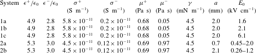
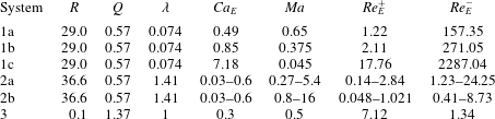
We first investigate drop dynamics in the Taylor regime, where the drops attain either a steady oblate or prolate shape depending on material properties. The Taylor regime was addressed in our recent work using both a small-deformation theory and axisymmetric boundary element simulations (Das & Saintillan Reference Das and Saintillan2017), and is primarily used here as a benchmark for our three-dimensional algorithm. Material properties in our simulations are chosen based on the experiments of Lanauze et al. (Reference Lanauze, Walker and Khair2015) for transient (system 1) and Salipante & Vlahovska (Reference Salipante and Vlahovska2010) for steady drop deformations (system 2) and are provided in table 1; corresponding dimensionless parameters are presented in table 2. Both of these experiments focused on oblate drops. We also consider the case of prolate deformations using one set of parameters from the experiments of Ha & Yang (Reference Ha and Yang2000a ) (system 3); their study, however, did not report all the material properties necessary to construct the five dimensional groups required in our model, so we set the electric capillary number to $Ca_{E}=0.3$ as in figure 10 of Lac & Homsy (Reference Lac and Homsy2007) and choose a finite value of $Ma=0.5$ for the Mason number.

Table 2.

Dimensionless parameters corresponding to the material properties of table 1: systems 1, 2 and 3 correspond to the experiments of Ha & Yang (Reference Ha and Yang2000a ), Salipante & Vlahovska (Reference Salipante and Vlahovska2010) and Lanauze et al. (Reference Lanauze, Walker and Khair2015), respectively.

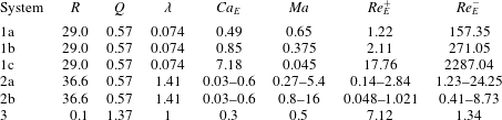
Figure 3(a) shows the transient deformation of an oblate drop corresponding to system 1a for an electric field strength of $E_{0}/E_{c}=0.49$ . Unsurprisingly, the axisymmetric boundary element method performs best in predicting the drop deformation when compared with experiments. Results from our three-dimensional simulations are shown for two different mesh resolutions ( $N_{d}=2$ and $3$ ) as a convergence test; we find as expected that the accuracy improves with increasing $N_{d}$ , and the results with $N_{d}=3$ are nearly identical to the predictions of the axisymmetric code. The classic small-deformation theories of Taylor (Reference Taylor1966) and Ajayi (Reference Ajayi1978) that neglect interfacial charge convection perform rather poorly; however, inclusion of charge convection in the theoretical model improves the results considerably (Das & Saintillan Reference Das and Saintillan2017).

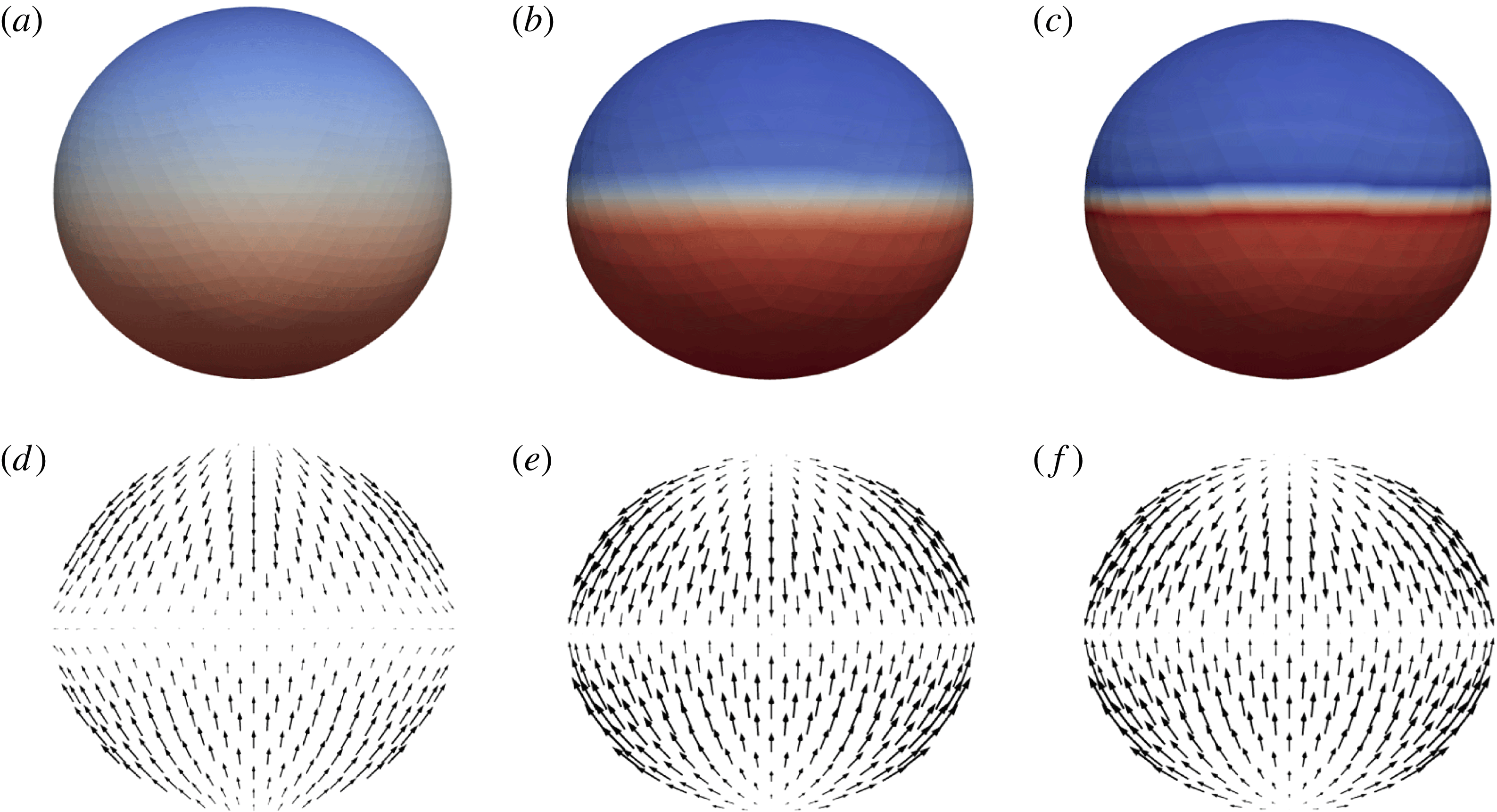
The case of system 1b, corresponding to a stronger applied field ( $E_{0}/E_{c}=0.64$ ), shows the same trends albeit with larger deformations in figure 3(b). While the boundary element simulations capture the transient and steady-state accurately, the performance of small-deformation theories is not as good as previously due to significant deformations. The surface charge distribution and fluid velocity obtained from the three-dimensional simulation for this case are illustrated at three different times in figure 4. As revealed by these snapshots, the interfacial velocity, which is directed from the poles towards the equator, causes transport of negative and positive charges towards the equatorial circumference of the drop, thereby inducing a sharp charge gradient across it. This gradient cannot be captured by small-deformation theories, as these employ truncated spherical harmonic expansions to represent variables; it is also challenging to capture numerically, especially as $E_{0}/E_{c}$ is increased further.

Figure 4.

Time evolution profiles of the surface charge density (a–c) and interfacial fluid velocity (d–f) in the case of system 1b in the Taylor regime at $t/\unicode[STIX]{x1D70F}_{MW}=1.0$ , $2.5$ and $4.0$ (a–f). See movie 1 in the supplementary online materials, available at https://doi.org/10.1017/jfm.2017.560, showing the dynamics and flow field in this case.

This is illustrated in figure 3(c), showing the case of system 1c with an even higher electric field of $E_{0}/E_{c}=1.86$ . There, the charge gradient across the interface becomes sharper and an actual discontinuity appears that triggers instabilities, leading to the termination of the simulations. Lanauze et al. (Reference Lanauze, Walker and Khair2015) were the first to discover this charge shock in their numerical work, and suggested that it might be an artefact of the axisymmetric nature of their boundary element simulations, which prevents transition to Quincke electrorotation. As we demonstrate here, the development of the charge shock in fact can occur in the Taylor regime, where it is due to the quadrupolar Taylor flow in the case of oblate drops that causes the sweeping of positive and negative charges towards the equator. The strength of this flow increases with electric field and is more pronounced for low-viscosity drops, leading to stronger shocks in these cases. While more analysis is required to understand the detailed structure of these shocks, we note that the Melcher–Taylor leaky dielectric model does not account for charge diffusion, which may have a regularizing effect in experiments. As expected, figure 3(c) shows a very poor performance of small-deformation theories in this regime, which are slightly improved by inclusion of charge convection but are unable to capture the charge discontinuity.

The case of prolate drop deformations corresponding to system 3 is shown in figure 3(d), where larger deformations are observed. The steady-state-deformation value reported in the experiments of Ha & Yang (Reference Ha and Yang2000a ), which did not specify the value of $Ma$ , is ${\mathcal{D}}=0.25$ ; the simulations of Lac & Homsy (Reference Lac and Homsy2007) with $Ma\rightarrow \infty$ reported ${\mathcal{D}}=0.22$ , while our simulations with $Ma=0.5$ predict ${\mathcal{D}}=0.27$ . No experimental data exist for the transient deformation, so we use axisymmetric simulations as the benchmark in this case. We find as expected that the three-dimensional simulations with $N_{d}=3$ perform best, especially when the mesh relaxation algorithm is used as deformations are significant. Unsurprisingly, the large drop deformation is poorly captured and underpredicted by the various small-deformation theories.

Figure 5.

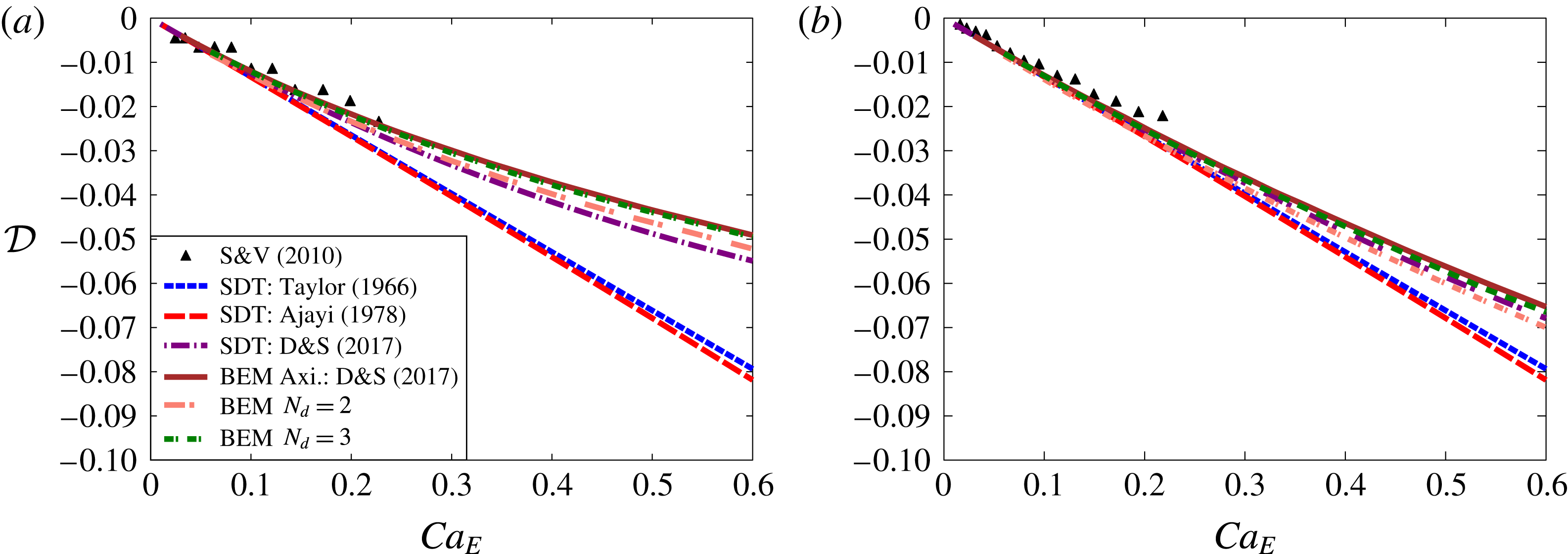
Steady drop deformation ${\mathcal{D}}$ as a function of electric capillary number $Ca_{E}$ for the parameters of: (a) system 2a and (b) system 2b. Boundary element (BEM) results are compared to the experiments of Salipante & Vlahovska (Reference Salipante and Vlahovska2010) and to various small-deformation theories (SDT).

We conclude the discussion of the Taylor regime by considering steady-state drop deformations corresponding to system 2, for which we compare our simulations with theoretical and experimental data in figure 5. Steady deformation values are shown for increasing values of electric capillary number $Ca_{E}$ for two different drop sizes of $a=0.7~\text{mm}$ and $a=2.1~\text{mm}$ . For a given value of $Ca_{E}$ , the smaller drop experiences a stronger electric field corresponding to a lower value of $Ma$ when compared to the larger drop. As a consequence, the small drop experiences stronger charge convection on its surface, which tends to reduce deformations as previously shown by other authors (Feng Reference Feng1999; Lanauze et al. Reference Lanauze, Walker and Khair2015). In consistency with previous results, the axisymmetric and three-dimensional simulations perform best followed by the small-deformation theory with convection (Das & Saintillan Reference Das and Saintillan2017). Since the effect of convection is weaker in the case of the larger drop, the small-deformation theories without convection do not deviate as much from the experimental data and simulation results as for the smaller drop.

4.2 Quincke regime

We now turn our attention to the electrorotation of drops in the Quincke regime, which is seen to occur when the applied field exceeds a certain critical value. For comparison with experiments, we use the parameter values provided by Salipante & Vlahovska (Reference Salipante and Vlahovska2010) but restrict ourselves to small drop sizes. We consider two different sets of material properties which are summarized in tables 3 and 4 and correspond to different viscosity ratios. The heuristic mesh relaxation algorithm of Loewenberg & Hinch (Reference Loewenberg and Hinch1996) is not included in the simulations in the Quincke regime, as we found that it caused numerical instabilities preventing the simulations from reaching steady state; as deformations tend to be fairly moderate when electrorotation takes place ( ${\mathcal{D}}\lesssim 0.1$ in the simulations shown below), we do not expect significant errors due to mesh distortion.

Table 3.

Material properties for system 2, corresponding to the experiments of Salipante & Vlahovska (Reference Salipante and Vlahovska2010) with a critical electric field of $E_{c}=2.68~\text{kV}~\text{cm}^{-1}$ . The permittivity and conductivity values for this system are given in table 1.

Table 4.

Dimensionless parameters corresponding to the material properties shown in table 3 for system 2, obtained from the experiments of Salipante & Vlahovska (Reference Salipante and Vlahovska2010).

Figure 6.

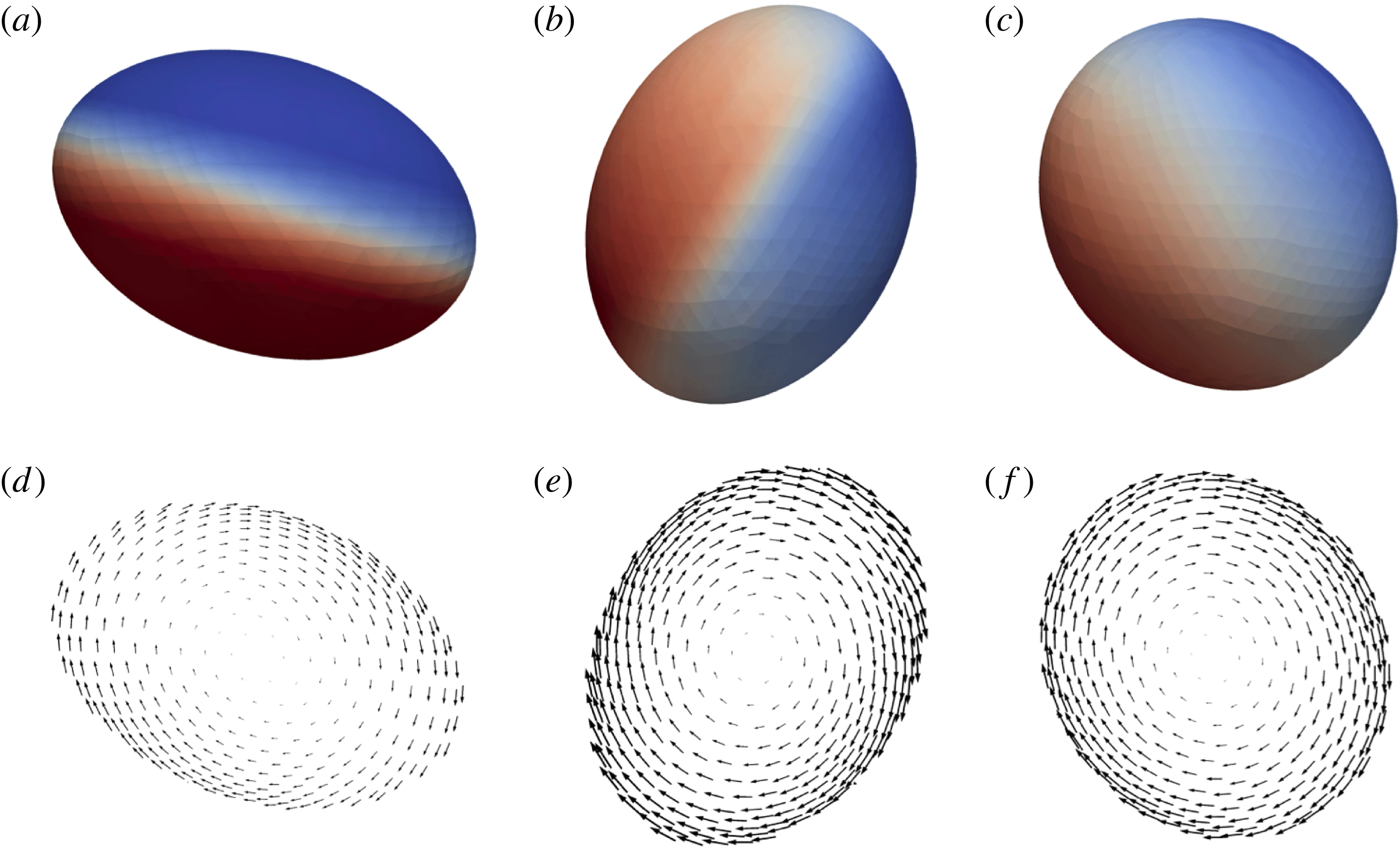
Time evolution profiles of the surface charge density (a–c) and interfacial fluid velocity (d–f) in the case of system 2c in the Quincke regime at $t/\unicode[STIX]{x1D70F}_{MW}=3.75$ , $5.25$ and $10.5$ (a–f). See supplementary online materials for movie 2 showing the dynamics and flow field in this case.

A typical simulation exhibiting Quincke rotation is illustrated in figure 6 in the case of system 2c for an initial drop radius of $a=1.25~\text{mm}$ and electric field $E_{0}/E_{c}=1.5$ , where $E_{c}$ is the critical electric field for the onset of rotation of a rigid sphere given in (2.16). The figure shows both the interfacial charge profile and interfacial velocity field at different times during the transient. Upon application of the field, the drop deforms towards an oblate shape similar to that found in the Taylor regime. This configuration, however, becomes unstable and leads to the rotation of the drop with respect to an arbitrary axis perpendicular to the field direction. 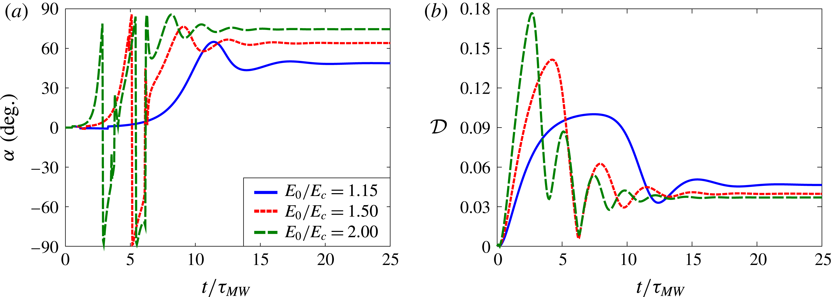As it rotates, the drop relaxes towards a more spherical shape as we characterize in more detail below, and ultimately reaches a steady shape with a tilt angle $\unicode[STIX]{x1D6FC}$ with respect to the horizontal plane. As is visible in figure 6, the charge profile is smoother than in the Taylor regime and is no longer axisymmetric, leading to a net electrostatic dipole that forms an angle with the field direction; the nature of the flow is also significantly different from the classic Taylor flow and appears to be primarily rotational. The transient dynamics is illustrated in more detail in figure 7, showing the tilt angle $\unicode[STIX]{x1D6FC}$ and deformation parameter ${\mathcal{D}}$ as functions of time for different electric field strengths. Oscillations in both $\unicode[STIX]{x1D6FC}$ and ${\mathcal{D}}$ are observed during the transient and are more significant in stronger fields, where the drop can undergo actual tumbling before its orientation stabilizes; similar time dynamics has also been reported in experiments (Salipante & Vlahovska Reference Salipante and Vlahovska2010) and theory (He et al. Reference He, Salipante and Vlahovska2013). In yet stronger fields, experiments have shown that the dynamics in some cases does not reach a steady state but instead exhibits chaotic tumbling and stretching of the drop (Salipante & Vlahovska Reference Salipante and Vlahovska2013); this regime was not captured in our simulations, which became unstable in very strong fields.

Figure 7.

(a) Tilt angle $\unicode[STIX]{x1D6FC}$ and (b) drop deformation parameter ${\mathcal{D}}$ as functions of time $t/\unicode[STIX]{x1D70F}_{MW}$ for system 2d with drop size $a=0.75$  mm and $Ca_{MW}=0.69$ . Stronger electric fields cause faster and more pronounced oscillations in the tilt angle and drop deformation.

Figure 8.

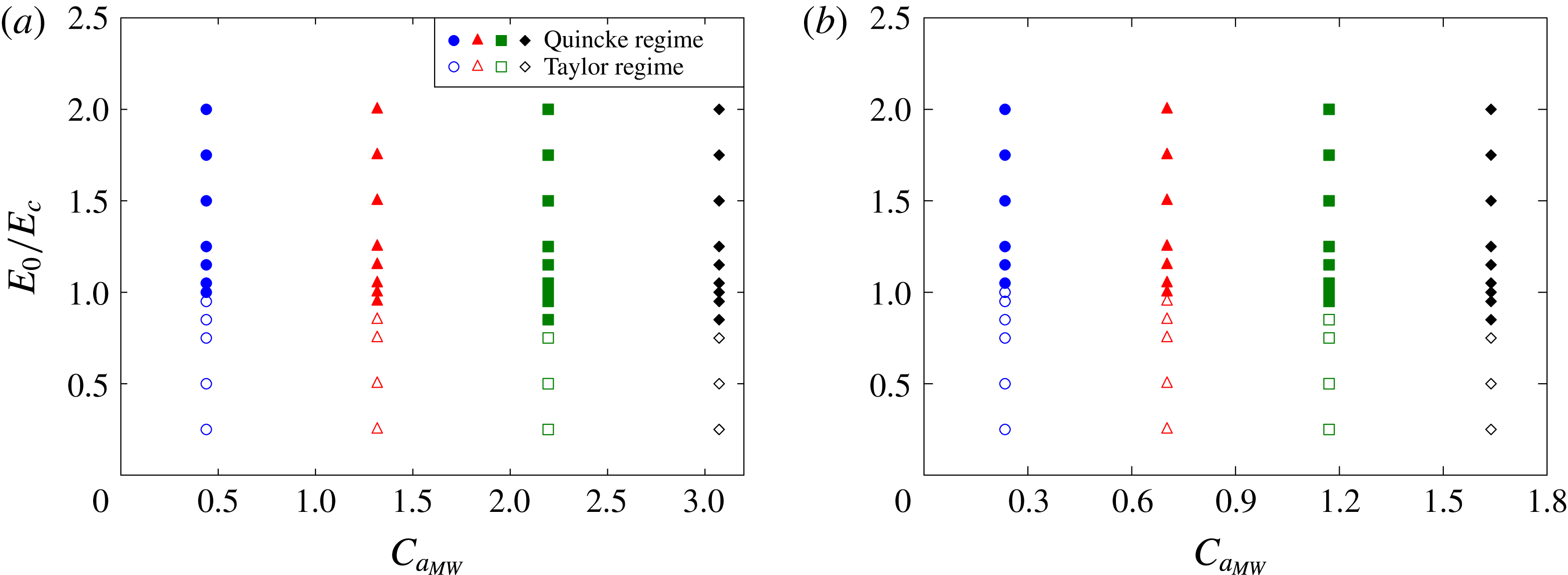
Phase diagram distinguishing the axisymmetric Taylor regime (empty symbols) from the Quincke electrorotation regime (filled symbols) for two different viscosity ratios: (a) $\unicode[STIX]{x1D706}=14.1$ and (b) $\unicode[STIX]{x1D706}=7.05$ . Different symbols are used to different values of $Ca_{MW}$ for consistency with the symbols used in figures 9 and 10.

The transition from the Taylor regime to the Quincke regime is characterized in more detail in figure 8 showing phase diagrams for systems 2c and 2d in the $(E_{0}/E_{c},Ca_{MW})$ plane, where we recall that for fixed material properties $Ca_{MW}$ is a measure of drop size. The case of a very viscous drop ( $\unicode[STIX]{x1D706}=14.1$ ) is shown in figure 8(a), where the critical electric field for the transition to electrorotation is found to be close to the value of $E_{c}$ for a rigid sphere, yet decreases slightly with increasing $Ca_{MW}$ . A small highly viscous drop is indeed expected to behave in the same way as a rigid particle. Increasing $Ca_{MW}$ (or equivalently, drop size) at a fixed value of $E_{0}/E_{c}$ leads to larger deformations in the Taylor regime, which causes an increase in the effective dipole induced inside the drop and thus has a destabilizing effect as demonstrated by the decrease in the critical electric field. A similar phase diagram is obtained at the lower viscosity ratio of $\unicode[STIX]{x1D706}=7.05$ in figure 8(b); decreasing $\unicode[STIX]{x1D706}$ , however, is found to slightly increase the threshold for Quincke rotation. All of these trends are consistent with the experimental data of Salipante & Vlahovska (Reference Salipante and Vlahovska2010).

Figure 9.

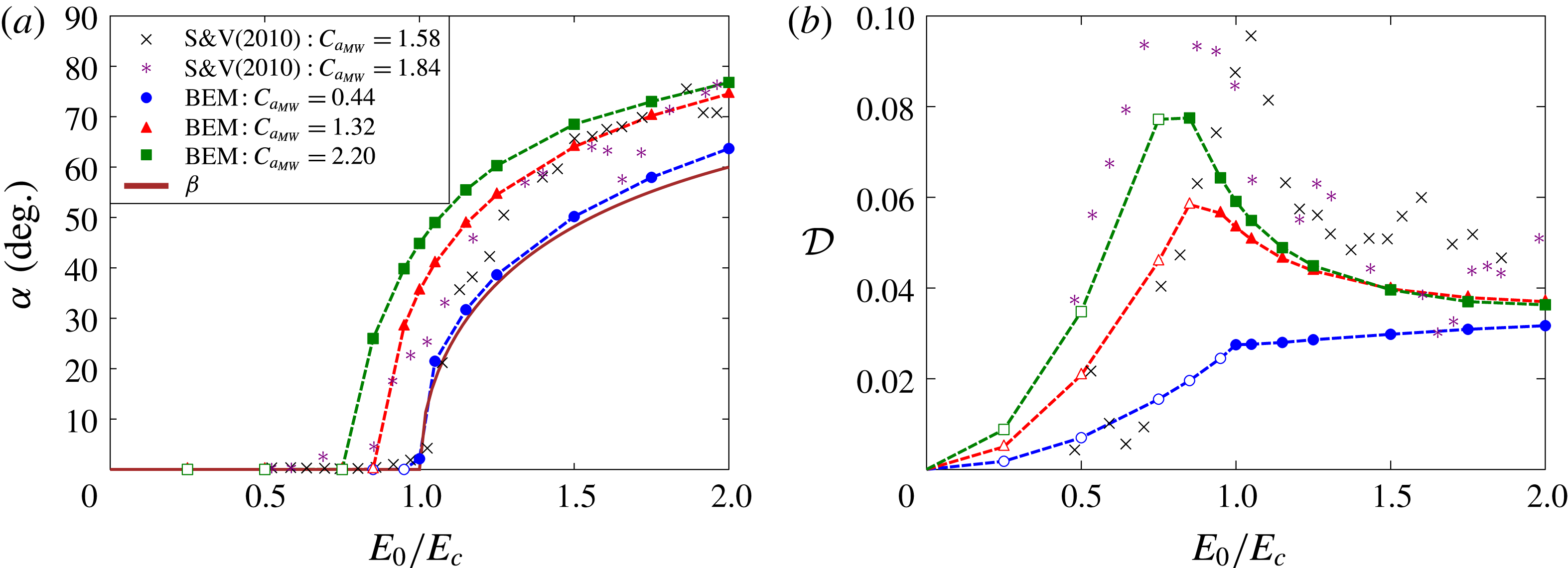
(a) Steady tilt angle $\unicode[STIX]{x1D6FC}$ and (b) drop deformation parameter ${\mathcal{D}}$ as functions of applied electric field strength $E_{0}/E_{c}$ for system 2c for different values of $Ca_{MW}$ . Boundary element (BEM) simulation results are compared with the experiments of Salipante & Vlahovska (Reference Salipante and Vlahovska2010) and with the theoretical predictions of He et al. (Reference He, Salipante and Vlahovska2013).

The steady-state tilt angle $\unicode[STIX]{x1D6FC}$ is shown as a function of electric field strength in figure 9(a) for system 2c, where it is also compared with the complementary of the angle between the steady dipole and applied electric field in the case of a rigid sphere, which we denote by $\unicode[STIX]{x1D6FD}$ (Salipante & Vlahovska Reference Salipante and Vlahovska2010):

In the Taylor regime, the tilt angle is zero as the drop shape is axisymmetric. As field strength increases, a supercritical pitchfork bifurcation is observed at the onset of rotation, with a value of $\unicode[STIX]{x1D6FC}$ that increases with $E_{0}/E_{c}$ and asymptotes towards $\unicode[STIX]{x03C0}/2$ in strong fields. Both angles $\unicode[STIX]{x1D6FC}$ and $\unicode[STIX]{x1D6FD}$ show similar trends as expected, especially in the case of weakly deformed drops ( $Ca_{MW}=0.44$ ) that behave like rigid spheres. Increasing drop size (or equivalently $Ca_{MW}$ ) causes the bifurcation to occur at lower field strengths in agreement with the phase diagram of figure 8. These trends also agree well with the experimental results of Salipante & Vlahovska (Reference Salipante and Vlahovska2010) and theoretical predictions of He et al. (Reference He, Salipante and Vlahovska2013) at similar values of $Ca_{MW}$ .

Corresponding values of the steady drop deformation ${\mathcal{D}}$ are shown in figure 9(b). Increasing field strength in the Taylor regime leads to stronger deformations in agreement with figure 5. The transition to electrorotation breaks this trend and leads to a relaxation of the drop towards a more spherical shape. This decrease in ${\mathcal{D}}$ with the onset of rotation can be rationalized as a result of a change in the nature of the flow. In the Taylor regime, the axisymmetric toroidal vortex flow illustrated in figure 4 is dominated by straining and causes the elongation of the drop in the equatorial plane; under Quincke rotation, the flow becomes primarily rotational and therefore has a weaker effect on drop shape. This qualitative change also has an impact on the charge distribution, which is much smoother in the Quincke regime than in the Taylor regime, thus reducing the effective dipole and the magnitude of electric stresses at a given field magnitude.

Figure 10.

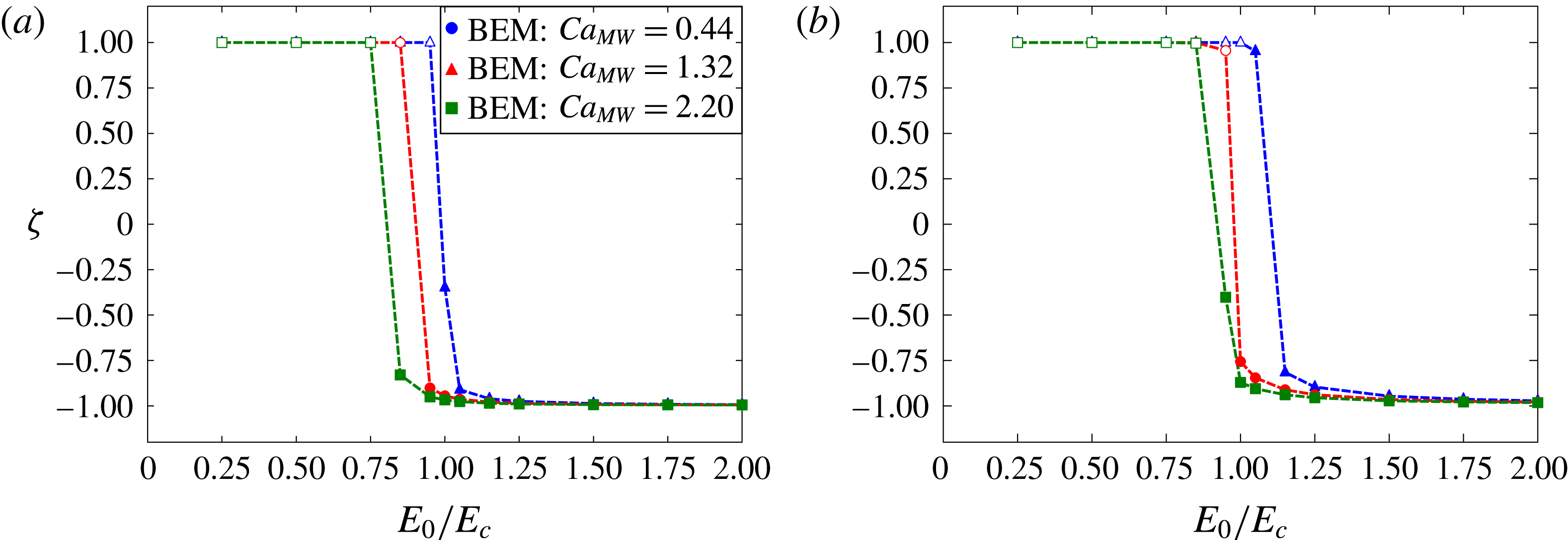
Parameter $\unicode[STIX]{x1D701}$ , defined in (4.3) and calculated at the position of the drop centroid for system 2c as a function of electric field strength for (a) $\unicode[STIX]{x1D706}=14.1$ and (b) $\unicode[STIX]{x1D706}=7.05$ . Values of $\unicode[STIX]{x1D701}$ close to $1$ or $-1$ describe flows dominated by either strain or rotation, respectively.

In order to quantify more precisely the nature of the flow inside the drop, we introduce a parameter $\unicode[STIX]{x1D701}$ as

where $\unicode[STIX]{x1D64E}=((\unicode[STIX]{x1D735}\boldsymbol{v}+\unicode[STIX]{x1D735}\boldsymbol{v}^{\text{T}}))/2$ and $\unicode[STIX]{x1D652}=((\unicode[STIX]{x1D735}\boldsymbol{v}-\unicode[STIX]{x1D735}\boldsymbol{v}^{\text{T}}))/2$ denote the rate-of-strain and rate-of-rotation tensors, respectively, which we evaluate at the centroid of the drop. With this definition, values of $\unicode[STIX]{x1D701}$ close to $+1$ and $-1$ describe flows dominated by strain and rotation, respectively. The dependence of $\unicode[STIX]{x1D701}$ on electric field strength in the steady state is shown in figure 10 for different values of $Ca_{MW}$ and for two viscosity ratios. In the Taylor regime, $\unicode[STIX]{x1D701}=1$ at the centre of the drop, which is to be expected for the axisymmetric Taylor flow. As the transition to electrorotation takes place, $\unicode[STIX]{x1D701}$ rapidly jumps to a value close to $-1$ , which indicates a drastic change in the nature of the flow. Note, however, that $\unicode[STIX]{x1D701}$ is not strictly $-1$ in the Quincke regime, implying that the flow retains a straining component; nonetheless, we find that $\unicode[STIX]{x1D701}\rightarrow -1$ as $E_{0}/E_{c}$ keeps increasing and the rotational component of the flow becomes more dominant.