1 Introduction
Steady shock reflection is an important flow phenomenon in supersonic flow. When an oblique shock wave, caused for instance by a wedge with deflection angle  $\unicode[STIX]{x1D703}_{w}$, reflects over a reflecting surface (such as a symmetry surface), either regular reflection (RR) or Mach reflection (MR) occurs. In regular reflection, a reflected shock wave is produced from the reflection point, leading to a two shock configuration. In Mach reflection, the reflected shock wave and the incident shock are connected to a strong shock wave called the Mach stem, forming a triple-shock configuration. A slipline, called a shear layer in viscous flow, is produced at the triple point.
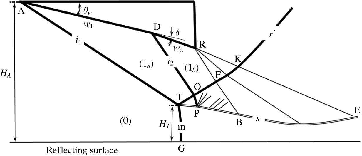
Shock reflection in steady supersonic flow has been extensively studied when the reflection is caused by a single incident shock wave (Ben-Dor Reference Ben-Dor2007) but is rarely considered in the case of multiple incident shock waves reflecting on a reflecting surface. Shock reflection by two incident shock waves may be found in applications such as the double-wedge problem, which produces two shock waves. However, double-wedge problems have been studied mainly in the context of shock interaction, without considering a reflecting surface at the interaction point of the two shock waves (Shah et al. Reference Shah, Martinez, Fernandez and Mourtos2008; Hu et al. Reference Hu, Gao, Myong, Dou and Khoo2010; Li, Zhu & Luo Reference Li, Zhu and Luo2014; Xiong, Zhu & Luo Reference Xiong, Zhu and Luo2016). Recently Guan, Bai & Wu (Reference Guan, Bai and Wu2018) considered shock reflection with double incident shock waves and with a common reflecting surface. The configuration they considered in the case of Mach reflection is shown in figure 1. The first incident shock wave ( $i_{1}$) has Mach reflection, its reflected shock wave intersects the second incident shock wave
 $(i_{2})$ at point O and this second incident shock wave is caused by an additional deflection
 $\unicode[STIX]{x1D6FF}$ of the wedge at point D. The transmitted part (OP) of the second incident shock wave reflects on the slipline at point P, creating an additional turning of the slipline. This additional turning was shown to have the effect of elevating the Mach stem. For convenience, shock reflection with a single incident shock wave will be called single-shock reflection and that with double incident shock waves (from one side) will be called double-shock reflection.
The work of Guan et al. (Reference Guan, Bai and Wu2018) was restricted to the effect of the second incident shock wave on the Mach reflection configuration of the first incident shock wave. The transition condition for double-shock reflection has not been considered. This transition problem is, however, particularly interesting and deserves to be studied, since there are two unexpected transition issues involved in double-shock reflection.
The first issue is the transition from regular to Mach reflection of each incident shock wave and, as discussed below, this issue is far more complex than single-shock reflection.
In case of Mach reflection, either the first incident shock wave may have Mach reflection, a situation called pre-Mach reflection here, or the second one has Mach reflection, a situation called post-Mach reflection here. Since there are three possible wave configurations (regular, pre-Mach and post-Mach reflections), the transition criteria are certainly much more difficult to obtain than for shock reflection of single-shock reflection, for which we have only two possible wave configurations. For instance, the pressure increasing effect of the second incident shock wave may cause the advance of Mach reflection of the first incident shock wave, leading to inverted Mach reflection under the usual von Neumann condition (Guan et al. Reference Guan, Bai and Wu2018). For inverted Mach reflection, the Mach stem is abnormally convex toward the upstream direction and the initial deflection angle of the slipline is negative (Henderson & Lozzi Reference Henderson and Lozzi1979; Hornung Reference Hornung1986; Roye, Henderson & Menikoff Reference Roye, Henderson and Menikoff1998; Ben-Dor et al. Reference Ben-Dor, Elperin, Li and Vasiliev1999; Hekiri & Emanuel Reference Hekiri and Emanuel2015). Due to this downstream pressure increasing effect, transition criteria are not simply related to solutions at the reflecting point, which is different from single-shock reflection.
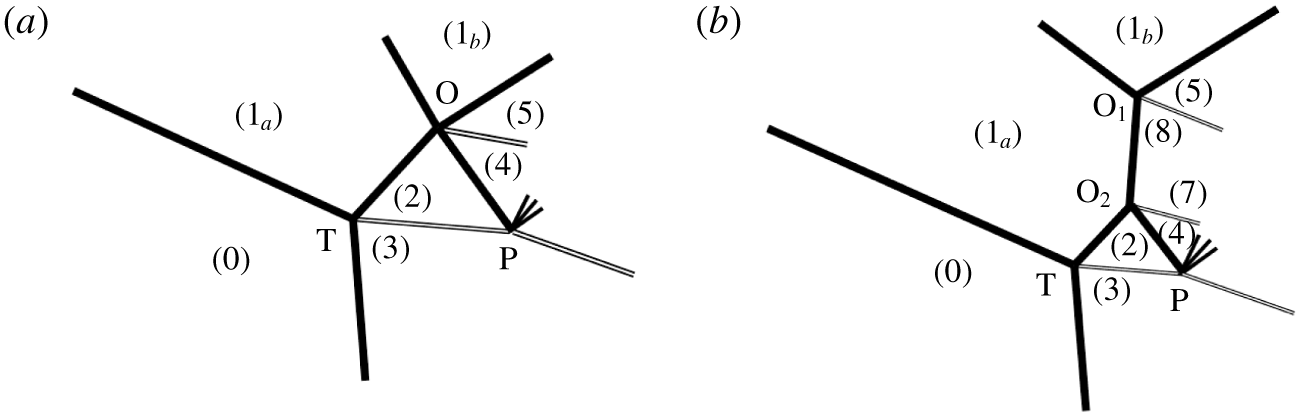
The second issue is the transition of shock interference types at point O for pre-Mach reflection displayed in figure 1. It is possible to have type I and type II shock interference patterns at point O, as displayed in figure 2. Before understanding the particular feature of this second issue, let us first recall the past studies about transition with regard to symmetric and asymmetric single-shock reflections.
Illustration of Mach reflection configuration with double incident shock waves.

First, consider symmetric single-shock reflection. Starting from the work by von Neumann (Reference von Neumann1943, Reference von Neumann1945), the transition criteria between regular and Mach reflection have attracted considerable attention. For a given inflow Mach number  $M_{0}$, there exists a
 $\unicode[STIX]{x1D703}_{w}=\unicode[STIX]{x1D703}_{w}^{(D)}$ above which the reflected shock wave detaches so that we necessarily have Mach reflection. Thus,
 $\unicode[STIX]{x1D703}_{w}=\unicode[STIX]{x1D703}_{w}^{(D)}(M_{0})$ is called the detachment condition for Mach reflection. For a given inflow Mach number
 $M_{0}$, there exists a
 $\unicode[STIX]{x1D703}_{w}=\unicode[STIX]{x1D703}_{w}^{(N)}$ below which the pressure increase across the incident and reflected shock waves cannot be balanced by the pressure increase across the Mach stem. Thus, we necessarily have regular reflection for
 $\unicode[STIX]{x1D703}_{w}<\unicode[STIX]{x1D703}_{w}^{(N)}$. Since von Neumann obtained this condition,
 $\unicode[STIX]{x1D703}_{w}=\unicode[STIX]{x1D703}_{w}^{(N)}(M_{0})$ was later on called the von Neumann condition. In the
 $M_{0}-\unicode[STIX]{x1D703}_{w}$ plane, the detachment criterion
 $\unicode[STIX]{x1D703}_{w}=\unicode[STIX]{x1D703}_{w}^{(D)}(M_{0})$ and von Neumann criterion
 $\unicode[STIX]{x1D703}_{w}=\unicode[STIX]{x1D703}_{w}^{(N)}(M_{0})$ are separated by a zone now called the dual solution domain, where both RR and MR are possible (Henderson & Lozzi Reference Henderson and Lozzi1975, Reference Henderson and Lozzi1979). Whether it is an RR or an MR in the dual solution domain depends on the history on which the actual steady flow is built (Hornung, Oertel & Sandeman Reference Hornung, Oertel and Sandeman1979; Ben-Dor et al. Reference Ben-Dor, Ivanov, Vasilev and Elperin2002; Ben-Dor Reference Ben-Dor2007; Hornung Reference Hornung1986, Reference Hornung2014).
For asymmetric single-shock reflection, where two wedges on opposite sides have different wedge angles and different wedge lengths, we also have RR and MR, and there is a double solution domain where both RR and MR are possible (Li, Chpoun & Ben-Dor Reference Li, Chpoun and Ben-Dor1999; Hu et al. Reference Hu, Kim, Myong and Cho2008). In this case, RR is also called type I shock interference and MR is also called type II shock interference.
Now we return back to double-shock reflection. The transition between type I and type II shock interference, for the shock interaction configuration at point O of figure 1, is apparently similar to the usual transition in asymmetrical single-shock reflection. However, two new features exist. For the first feature, in contrast to asymmetric single-shock reflection where the two opposite incident shock waves from the two wedges are prescribed, here, on one side, it is the reflected shock (TO) of the Mach configuration that plays the role of an incident shock wave. The question is whether the reflected shock wave (TO) is strong enough to cause type II shock interference at point O.
Mach reflection with two types of shock interference at point O. (a) Type I; (b) type II.

For the second feature, the reflected shock wave (TO) is subjected to influence of secondary Mach waves developed over the slipline (TP). These secondary waves have been studied by Gao & Wu (Reference Gao and Wu2010) in the case of single-shock Mach reflection. In the present case, these secondary waves should distort the reflected shock wave (TO) before this reflected shock wave intersects the second incident shock wave at point O. It is thus interesting to see whether these secondary Mach waves have a noticeable effect on the transition criteria for the shock interference pattern at point O. If this effect is demonstrated to be noticeable, then it offers the first case with transition criteria subjected to the influence of secondary waves. Past studies only considered the influence of primary waves on transition for single-shock reflection. For instance, Hillier (Reference Hillier2007) studied the influence of an upstream expansion wave on reflection type and Ben-Dor et al. (Reference Ben-Dor, Elperin, Li and Vasiliev1999) studied the influence of an artificially imposed downstream pressure on transition.
Hence, both transition issues for double-shock reflection are very complex and interesting, so that each of them deserves separate consideration. In this paper, we only consider the second issue (transition at point O), while the first issue (transition from regular, pre-Mach to post-Mach reflections) is left for possible future study.
The paper is organized as follows. In § 2, we will derive the conditions to have type I and II shock interferences at point O, by ignoring the secondary waves over the slipline and assuming the reflected shock wave to be straight.
In § 3 we consider the influence of the secondary waves on transition at point O. The secondary waves generated over the slipline will intersect the reflected shock wave (TO), producing reflected Mach waves that further reflect over the slipline. An analysis is thus conducted to show that these reflected Mach waves are weak enough to be omitted. With these reflected Mach waves omitted, we are able to derive an expression to estimate the modified shock angle of the reflected shock wave at point O and derive a correction to the transition criteria.
In § 4 we use computational fluid dynamics to support the theoretical results derived in §§ 2 and 3. We also display some results showing how the Mach stem height is affected by transition to type II shock interference at point O.
In the present study, we will ignore the real gas effect, including the high temperature gas effect and viscous effect. In the last part of § 4 we will briefly mention how these effects can be accounted for.
2 Transition criteria and double solution
Let the deflection angle  $\unicode[STIX]{x1D703}_{w}$, Mach number
 $M_{0}$ and additional deflection angle
 $\unicode[STIX]{x1D6FF}$ be such that the first incident shock wave has Mach reflection or inverted Mach reflection. We construct the necessary condition to have type I shock interference at point O, as shown in figure 2(a), and the sufficient condition to have type II shock interference at point O, as shown in figure 2(b). Hu et al. (Reference Hu, Kim, Myong and Cho2008) and Li et al. (Reference Li, Chpoun and Ben-Dor1999) have provided transition criteria for asymmetric single-shock reflection. Here, at point O, the transition is similar to that of asymmetric single-shock reflection, but is more complex in that one incident shock wave is here replaced by the reflected shock wave of a Mach reflection. In this section we assume the reflected shock wave to be straight.
2.1 Shock relations and triple point solution
To abbreviate expressions in the derivation of the transition criteria, we use
 $$\begin{eqnarray}\tan \unicode[STIX]{x1D703}=f_{\unicode[STIX]{x1D703}}(M_{u},\unicode[STIX]{x1D6FD}_{d}),\quad M_{d}=f_{M}(M_{u},\unicode[STIX]{x1D6FD}_{d}),\quad p_{d}=p_{u}f_{p}(M_{u},\unicode[STIX]{x1D6FD}_{d}),\end{eqnarray}$$
with
 $$\begin{eqnarray}\left.\begin{array}{@{}c@{}}\displaystyle f_{\unicode[STIX]{x1D703}}(M,\unicode[STIX]{x1D6FD})=\frac{2(M^{2}\sin ^{2}\unicode[STIX]{x1D6FD}-1)}{(M^{2}(\unicode[STIX]{x1D6FE}+\cos 2\unicode[STIX]{x1D6FD})+2)\tan \unicode[STIX]{x1D6FD}},\\ \displaystyle f_{M}(M,\unicode[STIX]{x1D6FD})=\sqrt{\frac{(\unicode[STIX]{x1D6FE}-1)M^{2}+2}{2\unicode[STIX]{x1D6FE}M^{2}\sin ^{2}\unicode[STIX]{x1D6FD}-(\unicode[STIX]{x1D6FE}-1)}+\frac{2M^{2}\cos ^{2}\unicode[STIX]{x1D6FD}}{(\unicode[STIX]{x1D6FE}-1)M^{2}\sin ^{2}\unicode[STIX]{x1D6FD}+2}},\\ \displaystyle f_{p}(M,\unicode[STIX]{x1D6FD})=1+\frac{2\unicode[STIX]{x1D6FE}}{\unicode[STIX]{x1D6FE}+1}(M^{2}\sin ^{2}\unicode[STIX]{x1D6FD}-1),\end{array}\right\}\end{eqnarray}$$
to denote the relations of oblique shock waves. Here, the subscripts  $u$ and
 $d$ denote upstream and downstream of the shock wave,
 $\unicode[STIX]{x1D6FD}$ denotes shock angle,
 $p$ denotes pressure,
 $\unicode[STIX]{x1D703}$ denotes flow deflection angle across the shock wave and
 $\unicode[STIX]{x1D6FE}$ denotes the ratio of specific heats. We take
 $\unicode[STIX]{x1D6FE}=1.4$ since we ignore the real gas effect. There are two solutions of
 $\unicode[STIX]{x1D6FD}$ for a given
 $\unicode[STIX]{x1D703}$, the smaller
 $\unicode[STIX]{x1D6FD}$ is for a weak shock wave and the bigger
 $\unicode[STIX]{x1D6FD}$ is for a strong shock wave. The local deflection flow angle
 $\unicode[STIX]{x1D703}$ is assumed to be positive if the deflection is towards the reflecting surface.
For each  $M_{u}$, the shock angle relation
 $\tan \unicode[STIX]{x1D703}=f_{\unicode[STIX]{x1D703}}(M_{u},\unicode[STIX]{x1D6FD}_{d})$ determines a maximum flow deflection angle
 $\unicode[STIX]{x1D703}_{max}(M_{u})$, given by
 $$\begin{eqnarray}\left.\begin{array}{@{}c@{}}\displaystyle \sin ^{2}\unicode[STIX]{x1D6FD}_{max}=\frac{1}{\unicode[STIX]{x1D6FE}M_{u}^{2}}\left[\frac{\unicode[STIX]{x1D6FE}+1}{4}M_{u}^{2}-1+\sqrt{(1+\unicode[STIX]{x1D6FE})\left(1+\frac{\unicode[STIX]{x1D6FE}-1}{2}M_{u}^{2}+\frac{\unicode[STIX]{x1D6FE}+1}{16}M_{u}^{4}\right)}\right],\\ \displaystyle \tan \unicode[STIX]{x1D703}_{max}=f_{\unicode[STIX]{x1D703}}(M_{u},\unicode[STIX]{x1D6FD}_{max}).\end{array}\right\}\end{eqnarray}$$
This maximum flow deflection angle  $\unicode[STIX]{x1D703}_{max}$ is also called the detachment angle.
As displayed in figure 1, the overall flow is divided into several uniform flow regions. The flow regions  $1_{a}$ and
 $1_{b}$ are the uniform flow region downstream of the first and second incident shock waves
 $i_{1}$ and
 $i_{2}$, and the flow parameters in these two regions are given by
 $$\begin{eqnarray}\tan \unicode[STIX]{x1D703}_{w}=f_{\unicode[STIX]{x1D703}}(M_{0},\unicode[STIX]{x1D6FD}_{1_{a}}),\quad M_{1_{a}}=f_{M}(M_{0},\unicode[STIX]{x1D6FD}_{1_{a}}),\quad p_{1_{a}}=p_{0}f_{p}(M_{0},\unicode[STIX]{x1D6FD}_{1_{a}}),\end{eqnarray}$$
and
 $$\begin{eqnarray}\tan \unicode[STIX]{x1D6FF}=f_{\unicode[STIX]{x1D703}}(M_{1_{a}},\unicode[STIX]{x1D6FD}_{1_{b}}),\quad M_{1_{b}}=f_{M}(M_{1_{a}},\unicode[STIX]{x1D6FD}_{1_{b}}),\quad p_{1_{b}}=p_{1_{a}}f_{p}(M_{1_{a}},\unicode[STIX]{x1D6FD}_{1_{b}}).\end{eqnarray}$$
Now consider the von Neumann triple point solution in the uniform flow regions 2 and 3.
The expressions to determine the flow parameters in regions  $2,3$ follow from the usual von Neumann three shock theory for the tripe point and are given by
 $$\begin{eqnarray}\left.\begin{array}{@{}c@{}}\tan (\unicode[STIX]{x1D703}_{w}-\unicode[STIX]{x1D703}_{2})=f_{\unicode[STIX]{x1D703}}(M_{1_{a}},\unicode[STIX]{x1D6FD}_{2}),\quad M_{2}=f_{M}(M_{1_{a}},\unicode[STIX]{x1D6FD}_{2}),\quad p_{2}=p_{1_{a}}f_{p}(M_{1_{a}},\unicode[STIX]{x1D6FD}_{2}),\\ \tan |\unicode[STIX]{x1D703}_{3}|=f_{\unicode[STIX]{x1D703}}(M_{0},\unicode[STIX]{x1D6FD}_{3}),\quad M_{3}=f_{M}(M_{0},\unicode[STIX]{x1D6FD}_{3}),\quad p_{3}=p_{0}f_{p}(M_{0},\unicode[STIX]{x1D6FD}_{3}),\\ \unicode[STIX]{x1D703}_{2}=\unicode[STIX]{x1D703}_{3},p_{2}=p_{3},\end{array}\right\}\end{eqnarray}$$
where  $\unicode[STIX]{x1D6FD}_{2}$ is solved for a weak shock wave and
 $\unicode[STIX]{x1D6FD}_{3}$ is solved for a strong shock wave.
2.2 The von Neumann condition for type I shock interference at point O
Now we determine the von Neumann condition  $\unicode[STIX]{x1D6FF}=\unicode[STIX]{x1D6FF}^{(N)}(M_{0},\unicode[STIX]{x1D703}_{w})$ for type I shock interference at point O. The von Neumann condition means that the length of shock
 $\text{O}_{1}\text{O}_{2}$ as displayed in figure 2(b) for shock II interference is infinitely small so that it can be seen as a straight strong shock wave. The von Neumann condition is satisfied when the pressure downstream of this infinitely small shock wave is balanced by the pressures in flow regions 4 and 5.
The flow deviation angle downstream of this infinitely small shock wave is first guessed to be  $\unicode[STIX]{x1D709}$. The flow deflection angle across this shock wave is thus
 $\unicode[STIX]{x1D709}-\unicode[STIX]{x1D703}_{w}$. The pressure downstream of this shock wave, denoted by
 $p_{78}$, is determined by
 $$\begin{eqnarray}\tan |\unicode[STIX]{x1D709}-\unicode[STIX]{x1D703}_{w}|=f_{\unicode[STIX]{x1D703}}(M_{1a},\unicode[STIX]{x1D6FD}_{78}),\quad M_{78}=f_{M}(M_{1_{a}},\unicode[STIX]{x1D6FD}_{78}),\quad p_{78}=p_{1_{a}}f_{p}(M_{1_{a}},\unicode[STIX]{x1D6FD}_{78}).\end{eqnarray}$$
The expression (2.7) is solved for a strong shock wave.
The flow deviation angle in regions 4 and 5 is also  $\unicode[STIX]{x1D709}$, so that the flow deflection angle across shock OP is
 $\unicode[STIX]{x1D709}-\unicode[STIX]{x1D703}_{2}$ and the flow deflection angle across shock OF is
 $\unicode[STIX]{x1D709}-(\unicode[STIX]{x1D703}_{w}+\unicode[STIX]{x1D6FF})<0$.
The flow parameters in regions 4 and 5 are thus given by
 $$\begin{eqnarray}\left.\begin{array}{@{}c@{}}\tan (\unicode[STIX]{x1D709}-\unicode[STIX]{x1D703}_{2})=f_{\unicode[STIX]{x1D703}}(M_{2},\unicode[STIX]{x1D6FD}_{4}),\quad M_{4}=f_{M}(M_{2},\unicode[STIX]{x1D6FD}_{4}),\quad p_{4}=p_{2}f_{p}(M_{2},\unicode[STIX]{x1D6FD}_{4}),\\ \tan |\unicode[STIX]{x1D709}-(\unicode[STIX]{x1D703}_{w}+\unicode[STIX]{x1D6FF})|=f_{\unicode[STIX]{x1D703}}(M_{1_{b}},\unicode[STIX]{x1D6FD}_{5}),\quad M_{5}=f_{M}(M_{1_{b}},\unicode[STIX]{x1D6FD}_{5}),\quad p_{5}=p_{1_{b}}f_{p}(M_{1_{b}},\unicode[STIX]{x1D6FD}_{5}).\end{array}\right\}\end{eqnarray}$$
For a given set of  $M_{0},p_{0}$ and
 $\unicode[STIX]{x1D703}_{w}$, and for an initially guessed value of
 $\unicode[STIX]{x1D6FF}$, the expressions (2.4) and (2.5) are first solved to give the flow parameters in region
 $1_{a}$ and region
 $1_{b}$. Then, the expressions in (2.6) are solved to give the flow parameters in region 2 and 3 as well as the flow deviation angle
 $\unicode[STIX]{x1D703}_{2}$. Then, for an assumed
 $\unicode[STIX]{x1D709}$, the expression (2.7) is solved for
 $p_{78}$. Finally, the expressions in (2.8) are solved for
 $p_{4}$ and
 $p_{5}$.
The von Neumann condition is here defined as the condition such that the pressure equilibrium condition
 $$\begin{eqnarray}p_{4}=p_{5}=p_{78}\end{eqnarray}$$
is met. Usually, the shock wave  $\text{O}_{1}\text{O}_{2}$ is strong enough so that one can use the pressure of normal shock wave
 $p_{n}=p_{1_{a}}f_{p}(M_{1_{a}},\unicode[STIX]{x03C0}/2)$ to approximate
 $p_{78}$.
The two conditions (2.9) allow us to determine the value of  $\unicode[STIX]{x1D709}$ and notably the von Neumann condition
 $\unicode[STIX]{x1D6FF}=\unicode[STIX]{x1D6FF}^{(N)}$ to have type I shock interference at point O.
2.3 Detachment condition for type II shock interference
Detachment condition for type II shock interference at point O is the condition that the flows in regions 4 and 5 (figure 2a) determined by the two transmitted shock waves (OP and OF in figure 1) cannot have a pressure balance unless at least one of these two shock waves detaches.
Now we give the method to obtain the detachment condition for point O to have type II shock interference.
For a given set of  $M_{0},p_{0}$ and
 $\unicode[STIX]{x1D703}_{w}$, and for an initial guess of
 $\unicode[STIX]{x1D6FF}$, the flow parameters in regions
 $1_{a},1_{b}$,
 $2,3$ are first solved by (2.4)–(2.6). Then, the flow parameters in regions
 $4,5$ (figure 2a) are determined by the following oblique shock wave relations for shocks OP and OF:
 $$\begin{eqnarray}\left.\begin{array}{@{}c@{}}\tan (\unicode[STIX]{x1D703}_{4}-\unicode[STIX]{x1D703}_{2})=f_{\unicode[STIX]{x1D703}}(M_{2},\unicode[STIX]{x1D6FD}_{4}),\quad M_{4}=f_{M}(M_{2},\unicode[STIX]{x1D6FD}_{4}),\quad p_{4}=p_{2}f_{p}(M_{2},\unicode[STIX]{x1D6FD}_{4}),\\ \tan (\unicode[STIX]{x1D703}_{w}+\unicode[STIX]{x1D6FF}-\unicode[STIX]{x1D703}_{5})=f_{\unicode[STIX]{x1D703}}(M_{1_{b}},\unicode[STIX]{x1D6FD}_{5}),\quad M_{5}=f_{M}(M_{1_{b}},\unicode[STIX]{x1D6FD}_{5}),\quad p_{5}=p_{1_{b}}f_{p}(M_{1_{b}},\unicode[STIX]{x1D6FD}_{5}),\end{array}\right\}\end{eqnarray}$$
where  $\unicode[STIX]{x1D703}_{4}$ and
 $\unicode[STIX]{x1D703}_{5}$ are unknown. Since both regions share the same slipline, we have the following further conditions to be met
 $$\begin{eqnarray}\unicode[STIX]{x1D703}_{4}=\unicode[STIX]{x1D703}_{5},\quad p_{4}=p_{5}.\end{eqnarray}$$
Hence, we have two restrictions, given in (2.11), while we have three unknowns  $\unicode[STIX]{x1D6FF}$,
 $\unicode[STIX]{x1D703}_{4}$ and
 $\unicode[STIX]{x1D703}_{5}$.
The detachment condition is met when  $\unicode[STIX]{x1D6FF}$ has such a value
 $\unicode[STIX]{x1D6FF}^{(D)}(M_{0},\unicode[STIX]{x1D703}_{w})$ that either
 $\unicode[STIX]{x1D703}_{4}-\unicode[STIX]{x1D703}_{2}$ or
 $\unicode[STIX]{x1D703}_{5}-(\unicode[STIX]{x1D703}_{w}+\unicode[STIX]{x1D6FF})$, with
 $\unicode[STIX]{x1D703}_{4}$ and
 $\unicode[STIX]{x1D703}_{5}$ determined by (2.4)–(2.6), equations (2.10) and (2.11), is equal to the detachment angle
 $\unicode[STIX]{x1D703}_{max}(M_{2})$ or
 $\unicode[STIX]{x1D703}_{max}(M_{1_{b}})$, determined by (2.3).
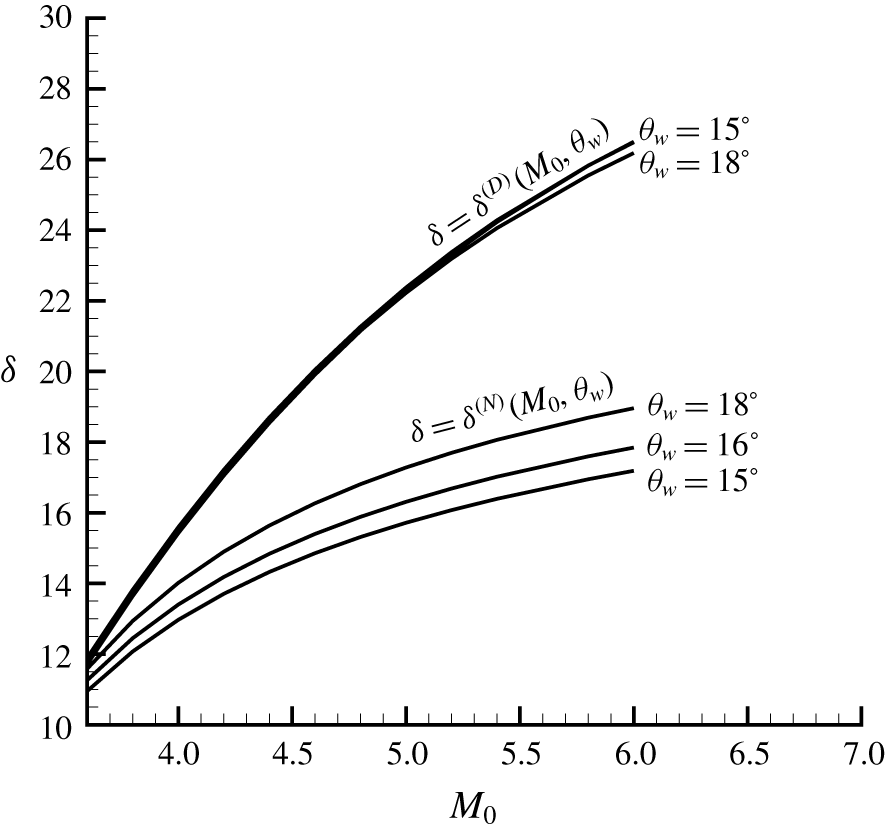
Transition criteria demonstrating double solution domain. Note that the curve  $\unicode[STIX]{x1D6FF}=\unicode[STIX]{x1D6FF}^{(D)}(M_{0},\unicode[STIX]{x1D703}_{w})$ at
 $\unicode[STIX]{x1D703}_{w}=16^{\circ }$ is close to that at
 $\unicode[STIX]{x1D703}_{w}=15^{\circ }$ so it is not shown.

2.4 Transition criteria and double solution domain
In figure 3, we display the von Neumann condition  $\unicode[STIX]{x1D6FF}=\unicode[STIX]{x1D6FF}^{(N)}(M_{0},\unicode[STIX]{x1D703}_{w})$ and detachment condition
 $\unicode[STIX]{x1D6FF}=\unicode[STIX]{x1D6FF}^{(D)}(M_{0},\unicode[STIX]{x1D703}_{w})$ in the plane
 $M_{0}-\unicode[STIX]{x1D6FF}$, for
 $\unicode[STIX]{x1D703}_{w}=15^{\circ }$,
 $16^{\circ }$ and
 $18^{\circ }$. We observe that the von Neumann condition is well below the detachment condition, so that we indeed have a double solution domain.
For given  $M_{0}$ and
 $\unicode[STIX]{x1D703}_{w}$ ensuring Mach reflection of the first incident shock wave, if
 $\unicode[STIX]{x1D6FF}<\unicode[STIX]{x1D6FF}^{(N)}(M_{0},\unicode[STIX]{x1D703}_{w})$, we necessarily have type I shock interference at point O and if
 $\unicode[STIX]{x1D6FF}>\unicode[STIX]{x1D6FF}^{(D)}(M_{0},\unicode[STIX]{x1D703}_{w})$, we necessarily have type II shock interference at point O. A double solution exists for
 $\unicode[STIX]{x1D6FF}^{(N)}(M_{0},\unicode[STIX]{x1D703}_{w})<\unicode[STIX]{x1D6FF}<\unicode[STIX]{x1D6FF}^{(D)}(M_{0},\unicode[STIX]{x1D703}_{w})$.
It is interesting to note that, when  $\unicode[STIX]{x1D703}_{w}$ is increased, the von Neumann condition is elevated but the detachment condition is lowered, so that the double solution domain is narrowed. For a fixed
 $\unicode[STIX]{x1D703}_{w}$, if the Mach number is sufficiently small, the double solution domain may be so narrow as to be non-existent.
3 Influence of secondary waves generated over the slipline
In § 2, we have derived transition criteria by assuming the reflected shock wave to be straight. In this section, we consider the influence of secondary waves produced from the slipline (Gao & Wu Reference Gao and Wu2010). These secondary waves should curve the reflected shock wave to alter the transition criteria. We conduct a theoretical analysis to see whether the effect of secondary waves is strong or weak. In the following we will repeatedly use the Prandtl–Meyer function
 $$\begin{eqnarray}\unicode[STIX]{x1D708}(M)=\sqrt{\frac{\unicode[STIX]{x1D6FE}+1}{\unicode[STIX]{x1D6FE}-1}}\arctan \sqrt{\frac{\unicode[STIX]{x1D6FE}-1}{\unicode[STIX]{x1D6FE}+1}(M^{2}-1)}-\arctan \sqrt{M^{2}-1}\end{eqnarray}$$
and the common factor  $\unicode[STIX]{x1D717}(M)=1+((\unicode[STIX]{x1D6FE}-1)/2)M^{2}$ found in isentropic relations of gas dynamics.
3.1 Analysis of the wave structure due to secondary waves
The mechanism by which secondary waves are generated over the slipline for single-shock Mach reflection has been explained by Gao & Wu (Reference Gao and Wu2010).
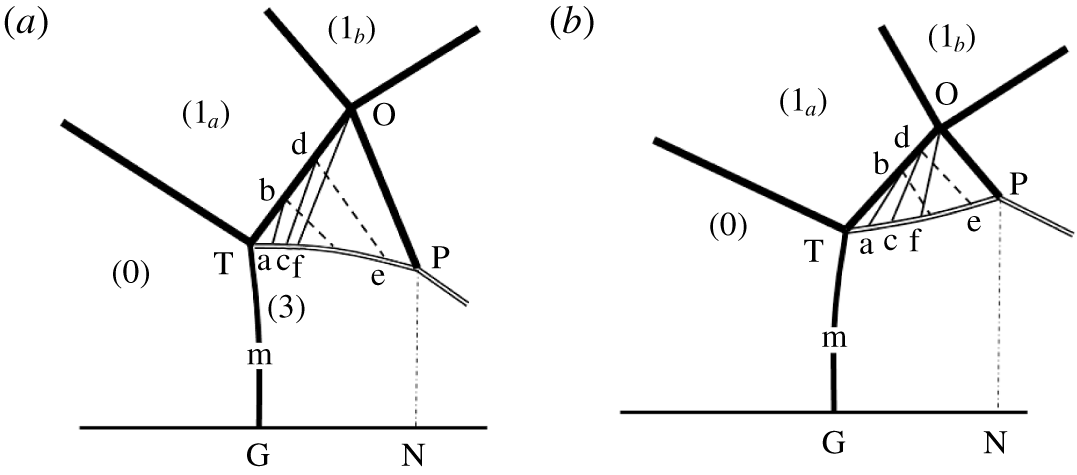
As can be seen in figure 4(a), the flow duct between TP and GN (flow duct downstream of the Mach stem) is convergent so that the pressure decreases along the flow direction according to the quasi-one-dimensional flow theory. To balance this pressure decrease on both sides of the slipline TP, the pressure in the flow just above this slipline should also decrease along the flow streamline. In the case of single-shock reflection, this pressure decrease is shown in figure 5 of Gao & Wu (Reference Gao and Wu2010). This pressure decrease induces expansion Mach waves, such as ‘ab’, ‘cd’ and ‘fO’ in figure 4(a), over the slipline TP. These expansion waves intersect the reflected shock wave to weaken it, so its shock angle is decreased at point O. This is a situation similar to that studied by Gao & Wu (Reference Gao and Wu2010).
Secondary waves over the slipline. (a) Usual Mach reflection; (b) inverted Mach reflection. The secondary wave cd reflects on the reflected shock wave to produce a reflected wave de. The point f produces a secondary wave that intersects the point O.

There is another situation not considered by Gao & Wu (Reference Gao and Wu2010). For double-shock Mach reflection, inverted Mach reflection is possible (Guan et al. Reference Guan, Bai and Wu2018). For inverted Mach reflection, the initial segment of slipline deflects towards the upward direction so that the quasi-one-dimensional duct downstream of the Mach stem is initially divergent. Figure 4(b) displays the wave structure for inverted Mach reflection. The flow duct between TP and GN (flow duct downstream of the Mach stem) is divergent so that the pressure increases along the flow direction. To balance this pressure increase on both sides of the slipline TP, the pressure in the flow just above this slipline should also increase along the flow streamline. This pressure increase induces compressive Mach waves, such as ‘ab’, ‘cd’ and ‘fO’ in figure 4(b), over the slipline TP. These compressive waves intersect the reflected shock wave to strengthen it, so its shock angle is increased at point O.
The interaction of an expansion or compressive wave, such as cd in figure 4(a,b), with the reflected shock wave (TO) normally produces reflected waves, such as de in figure 4(a,b). These reflected waves further intersect and reflect over the slipline (TP), so that we have two families of Mach waves that interact and reflect between the slipline (TP) and the reflected shock wave (TO). An analytical model accounting for these detailed wave interacting structures is too complex. Luckily, the reflected Mach wave (such as de) is one order of magnitude weaker than the incident Mach wave (such as cd) that causes it, as will be shown in § 3.2.
3.2 The reason why the reflected Mach wave can be omitted
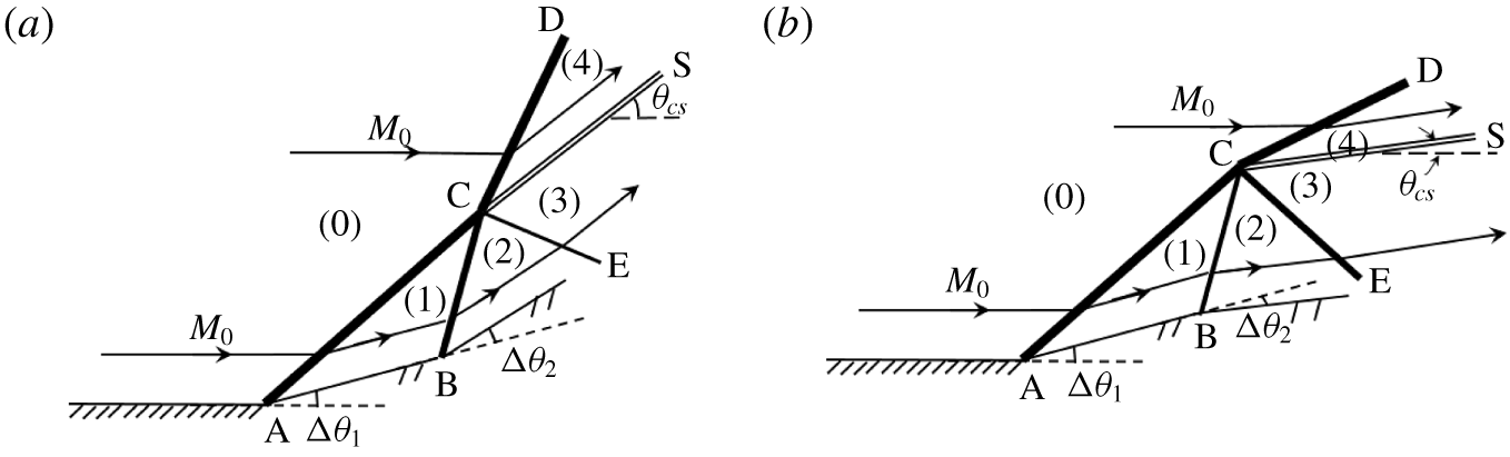
To show that the reflected wave of a Mach wave from a shock wave is of negligible importance, we consider the wave configuration as displayed in figure 5. In this configuration, the primary shock wave AC is triggered by the wedge with initial angle  $\unicode[STIX]{x0394}\unicode[STIX]{x1D703}_{1}=\unicode[STIX]{x1D703}_{1}-\unicode[STIX]{x1D703}_{0}=\unicode[STIX]{x1D703}_{1}$ assuming
 $\unicode[STIX]{x1D703}_{0}=0$. The downstream compressive Mach wave or expansion wave CB is generated by an additional deflection angle
 $\unicode[STIX]{x0394}\unicode[STIX]{x1D703}_{2}=\unicode[STIX]{x1D703}_{2}-\unicode[STIX]{x1D703}_{1}$. The wave CE is produced by the reflection of CB over the shock wave AC. Now, we want to show that the reflected wave CE is at least one order of magnitude weaker than the incident wave CB in terms of the pressure variation across the wave, under a wide parameter range and assuming the gas is perfect. In the following, the flow deflection angle
 $\unicode[STIX]{x1D703}$ is assumed positive if it is clockwise.
Interaction of a Mach wave with a shock wave. (a) The Mach wave is compressive; (b) the Mach wave is expansive.

With  $\unicode[STIX]{x1D703}_{1}-\unicode[STIX]{x1D703}_{0}$ and
 $M_{0}$ prescribed, the flow parameters in region 1 follow from the oblique shock wave relations
 $$\begin{eqnarray}\tan (\unicode[STIX]{x1D703}_{1}-\unicode[STIX]{x1D703}_{0})=f_{\unicode[STIX]{x1D703}}(M_{0},\unicode[STIX]{x1D6FD}_{1}),\quad M_{1}=f_{M}(M_{0},\unicode[STIX]{x1D6FD}_{1}),\quad p_{1}=p_{0}f_{p}(M_{0},\unicode[STIX]{x1D6FD}_{1}).\end{eqnarray}$$
With  $M_{1}$ given by (3.1) and with
 $\unicode[STIX]{x1D703}_{2}-\unicode[STIX]{x1D703}_{1}$ prescribed, the flow parameters of region 2 can be solved by
 $$\begin{eqnarray}\tan (\unicode[STIX]{x1D703}_{2}-\unicode[STIX]{x1D703}_{1})=f_{\unicode[STIX]{x1D703}}(M_{1},\unicode[STIX]{x1D6FD}_{2}),\quad M_{2}=f_{M}(M_{1},\unicode[STIX]{x1D6FD}_{2}),\quad p_{2}=p_{1}f_{p}(M_{1},\unicode[STIX]{x1D6FD}_{2}),\end{eqnarray}$$
for  $\unicode[STIX]{x1D703}_{2}-\unicode[STIX]{x1D703}_{1}>0$ and by
 $$\begin{eqnarray}|\unicode[STIX]{x1D703}_{2}-\unicode[STIX]{x1D703}_{1}|=\unicode[STIX]{x1D708}(M_{2})-\unicode[STIX]{x1D708}(M_{1}),\quad p_{2}=p_{1}\left(\frac{\unicode[STIX]{x1D717}(M_{1})}{\unicode[STIX]{x1D717}(M_{2})}\right)^{\unicode[STIX]{x1D6FE}/(\unicode[STIX]{x1D6FE}-1)},\end{eqnarray}$$
for  $\unicode[STIX]{x1D703}_{2}-\unicode[STIX]{x1D703}_{1}<0$.
The flow in region 3 is separated from the flow in region 4 by a slipline of deviation angle  $\unicode[STIX]{x1D703}_{cs}$. The flow streams in regions 3 and 4 are both parallel to the slipline and their pressures are continuous across this slipline, thus
 $$\begin{eqnarray}\left.\begin{array}{@{}c@{}}p_{3}=p_{4},\\ \unicode[STIX]{x1D703}_{3}=\unicode[STIX]{x1D703}_{4}=\unicode[STIX]{x1D703}_{cs}.\end{array}\right\}\end{eqnarray}$$
The reflected wave CE can be compressive or expansive, thus the flow parameters in region 3 are given by
 $$\begin{eqnarray}\tan |\unicode[STIX]{x1D703}_{3}-\unicode[STIX]{x1D703}_{2}|=f_{\unicode[STIX]{x1D703}}(M_{2},\unicode[STIX]{x1D6FD}_{3}),\quad M_{3}=f_{M}(M_{2},\unicode[STIX]{x1D6FD}_{3}),\quad p_{3}=p_{2}f_{p}(M_{2},\unicode[STIX]{x1D6FD}_{3}),\end{eqnarray}$$
or
 $$\begin{eqnarray}|\unicode[STIX]{x1D703}_{3}-\unicode[STIX]{x1D703}_{2}|=\unicode[STIX]{x1D708}(M_{3})-\unicode[STIX]{x1D708}(M_{2}),\quad p_{3}=p_{2}\left(\frac{\unicode[STIX]{x1D717}(M_{2})}{\unicode[STIX]{x1D717}(M_{3})}\right)^{\unicode[STIX]{x1D6FE}/(\unicode[STIX]{x1D6FE}-1)}.\end{eqnarray}$$
The flow parameters in region 4 are given by
 $$\begin{eqnarray}\tan \unicode[STIX]{x1D703}_{4}=f_{\unicode[STIX]{x1D703}}(M_{0},\unicode[STIX]{x1D6FD}_{4}),\quad M_{4}=f_{M}(M_{0},\unicode[STIX]{x1D6FD}_{4}),\quad p_{4}=p_{0}f_{p}(M_{0},\unicode[STIX]{x1D6FD}_{4}).\end{eqnarray}$$
If (3.5) ensures (3.4) is satisfied, CE is compressive. If (3.6) can ensure (3.4) is satisfied, CE is expansive.
We choose the parameter range  $3<M_{0}<20$ and
 $10^{\circ }<\unicode[STIX]{x1D703}_{1}-\unicode[STIX]{x1D703}_{0}=\unicode[STIX]{x1D703}_{1}<30^{\circ }$ and solve (3.1)–(3.7) to get
 $p_{1},p_{2}$ and
 $p_{3}$. We use the ratio
 $$\begin{eqnarray}r_{p}=\frac{p_{3}-p_{2}}{p_{2}-p_{1}}\end{eqnarray}$$
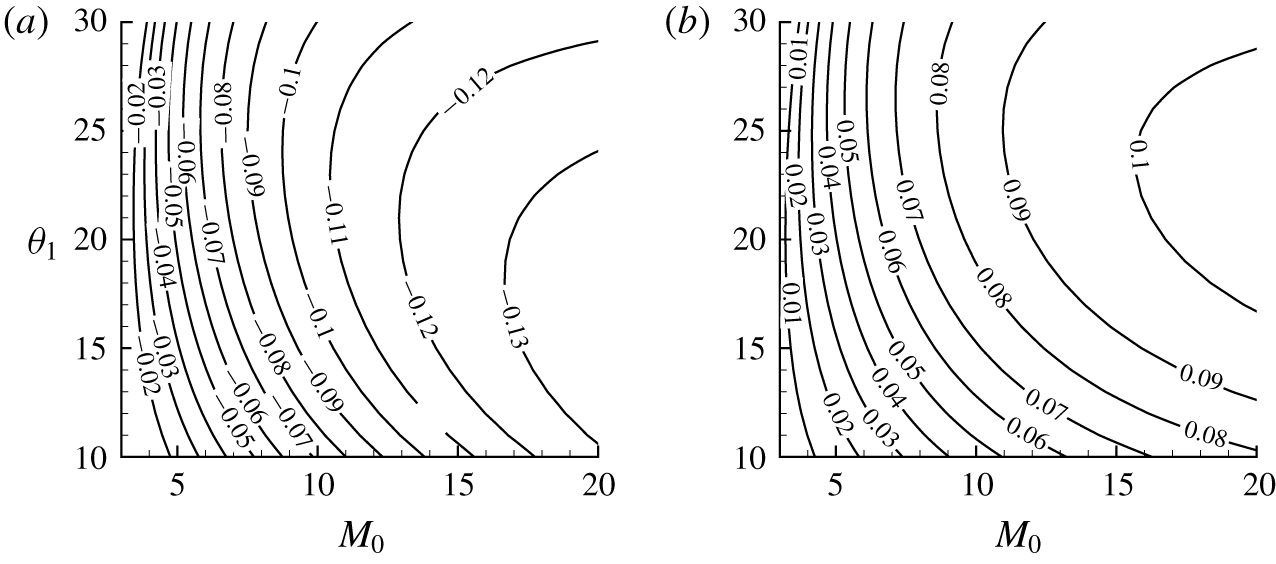
to measure the strength of the reflected wave CE relative to the strength of the incident wave CB. The contours of the iso-values for the ratio  $r$ are displayed in figure 6.
The contour lines for  $(p_{3}-p_{2})/(p_{2}-p_{1})$ in the
 $M_{0}$–
 $\unicode[STIX]{x1D703}_{1}$ plane with positive and negative
 $\unicode[STIX]{x0394}\unicode[STIX]{x1D703}_{2}$. (a) Positive,
 $\unicode[STIX]{x0394}\unicode[STIX]{x1D703}_{2}=1^{\circ }$, (b) negative,
 $\unicode[STIX]{x0394}\unicode[STIX]{x1D703}_{2}=-1^{\circ }$.

As is clear from figure 6,  $|r_{p}|\ll 1$ for a wide range of parameter range in the
 $M_{0}$–
 $\unicode[STIX]{x1D703}_{1}$ plane. Thus, as a first-order approximation, the reflected wave CE can be omitted.
3.3 Model for the shock angle  $\unicode[STIX]{x1D6FD}_{2}^{(O)}$ of the reflected shock wave

Now, with the reflected waves (such as de in figure 4) neglected, we give a model to estimate the shock angle  $\unicode[STIX]{x1D6FD}_{2}^{(O)}$ at point O due to influence of secondary waves (such as cd in figure 4) generated from the slipline. Without these secondary waves we have
 $\unicode[STIX]{x1D6FD}_{2}^{(O)}=\unicode[STIX]{x1D6FD}_{2}^{(T)}$.
Let f be the point on the slipline such that the secondary wave from this point intersects the interaction point O. Since fO is a Mach wave, here assumed to be straight, we have
 $$\begin{eqnarray}\frac{y_{O}-y_{f}}{x_{O}-x_{f}}=\tan (\unicode[STIX]{x1D707}_{2}-\unicode[STIX]{x1D703}_{2}),\end{eqnarray}$$
where  $\unicode[STIX]{x1D707}_{2}=\arcsin (1/M_{2})$ is the Mach angle and
 $\unicode[STIX]{x1D703}_{2}$ is the flow deflection angle in region 2. Assuming the secondary waves to be weak enough we may approximate
 $\unicode[STIX]{x1D707}_{2}=\unicode[STIX]{x1D707}_{2}^{(T)}=\arcsin (1/M_{2}^{(T)})$ and
 $\unicode[STIX]{x1D703}_{2}=\unicode[STIX]{x1D703}_{2}^{(T)}$. The approximate expressions for estimating
 $x_{O}$ and
 $y_{O}$ of Guan et al. (Reference Guan, Bai and Wu2018) are used here.
For  $\unicode[STIX]{x1D703}_{2}^{(T)}>0$ (usual Mach stem) or
 $\unicode[STIX]{x1D703}_{2}^{(T)}<0$ (inverted Mach stem), the initial part of the quasi-one-dimensional flow duct between the slipline and the reflecting surface is convergent or divergent, leading to a pressure decrease or increase described by the isentropic flow expression
 $$\begin{eqnarray}\frac{\text{d}p_{s}^{-}}{p_{s}^{-}}=\frac{\unicode[STIX]{x1D6FE}(M_{s}^{-})^{2}}{1-(M_{s}^{-})^{2}}\frac{\text{d}H_{s}}{H_{s}},\end{eqnarray}$$
where  $p_{s}^{-}$ and
 $M_{s}^{-}$ are the average pressure and average Mach number of the flow in the duct and
 $H_{s}$ is the height of the slipline (or quasi-one-dimensional flow duct).
The pressure decrease or increase in the duct is balance by the same change of pressure over the slipline, producing expansive or compressive secondary waves. Across the waves, the pressure meets the following Mach wave relation
 $$\begin{eqnarray}\frac{\text{d}p_{s}^{+}}{p_{s}^{+}}=-\frac{\unicode[STIX]{x1D6FE}(M_{s}^{+})^{2}\,\text{d}\unicode[STIX]{x1D703}_{s}}{\sqrt{(M_{s}^{+})^{2}-1}}.\end{eqnarray}$$
In (3.10),  $p_{s}^{+}$ and
 $M_{s}^{+}$ are pressure and Mach number over the slipline (TP),
 $\unicode[STIX]{x1D703}_{s}$ is the slipline deflection angle related to
 $H_{s}$ by
 $\tan \unicode[STIX]{x1D703}_{s}=-\text{d}H_{s}/\text{d}x$.
Bai & Wu (Reference Bai and Wu2017) set  $p=p_{s}^{+}$ and solve the above slipline model nonlinearly to obtain the following expression for
 $H_{s}$:
 $$\begin{eqnarray}\frac{H_{s}}{H_{T}}=\frac{M_{m}^{-}N^{-(\unicode[STIX]{x1D6FE}+1)/2\unicode[STIX]{x1D6FE}}}{\sqrt{\displaystyle \frac{2}{\unicode[STIX]{x1D6FE}-1}(\unicode[STIX]{x1D717}(M_{m}^{-})N^{-(\unicode[STIX]{x1D6FE}-1)/\unicode[STIX]{x1D6FE}}\unicode[STIX]{x1D717}(M_{s}^{+})-1)}}(\unicode[STIX]{x1D717}(M_{s}^{+}))^{(\unicode[STIX]{x1D6FE}+1)/2(\unicode[STIX]{x1D6FE}-1)}.\end{eqnarray}$$
Here, the subscript  $m$ means the solution at the inlet of the flow duct (taken as the arithmetic average of the normal shock wave solution and the triple point solution in region 3),
 $N=(p_{2}^{T}/p_{m}^{-})(\unicode[STIX]{x1D717}(M_{2}^{(T)}))^{\unicode[STIX]{x1D6FE}/(\unicode[STIX]{x1D6FE}-1)}$ and
 $M_{s}^{+}$ is given by the Prandtl–Meyer relation
 $\unicode[STIX]{x1D708}(M_{s}^{+})=\unicode[STIX]{x1D703}_{s}-\unicode[STIX]{x1D703}_{s}^{(T)}+\unicode[STIX]{x1D708}(M_{2}^{(T)})$.
For each  $x$, equation (3.11) is solved to get
 $H_{s}=H_{s}(x)$ and
 $\unicode[STIX]{x1D703}_{s}=-\arctan \,\text{d}H_{s}/\text{d}x$. The point f is achieved once
 $x$ and the resulting
 $y(=H_{s})$ meet (3.8). We set
 $$\begin{eqnarray}\unicode[STIX]{x1D703}_{f}=\unicode[STIX]{x1D703}_{s}(x_{f}).\end{eqnarray}$$
The local flow deflection angle at any point (such as d) on the reflected shock wave is assumed to be equal to the deflection angle of the slipline at the point (such as c) connecting to the reflected shock wave by the secondary wave (such as cd). Thus,  $\unicode[STIX]{x1D703}_{2}^{(O)}=\unicode[STIX]{x1D703}_{f}$ and the shock angle
 $\unicode[STIX]{x1D6FD}_{2}^{(O)}$ at point O is given by
 $$\begin{eqnarray}\tan (\unicode[STIX]{x1D703}_{f}-\unicode[STIX]{x1D703}_{1_{a}})=f_{\unicode[STIX]{x1D703}}(M_{1_{a}},\unicode[STIX]{x1D6FD}_{2}^{(O)}).\end{eqnarray}$$
3.4 Modified transition criteria and influence of secondary waves
Once  $\unicode[STIX]{x1D703}_{2}^{(O)}=\unicode[STIX]{x1D703}_{f}$ and
 $\unicode[STIX]{x1D6FD}_{2}^{(O)}$ are obtained from (3.12) and (3.13), it is very simple to obtain a correction for the secondary wave effect to the transition criteria. To obtain a correction for secondary waves to the transition criteria, we replace
 $\unicode[STIX]{x1D703}_{2}$ by
 $\unicode[STIX]{x1D703}_{2}^{(O)}=\unicode[STIX]{x1D703}_{f}$ in the expressions (2.8) and (2.10) to obtain a correction to the transition criteria. The corrected von Neumann and detachment conditions for
 $\unicode[STIX]{x1D6FF}$ are denoted with
 $\unicode[STIX]{x1D6FF}_{sw}^{(N)}$ and
 $\unicode[STIX]{x1D6FF}_{sw}^{(D)}$, which will be compared to the non-corrected transition criteria
 $\unicode[STIX]{x1D6FF}^{(N)}$ and
 $\unicode[STIX]{x1D6FF}^{(D)}$.
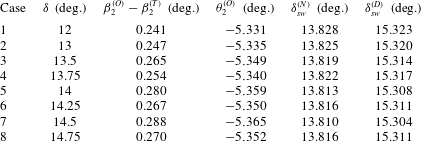
For an inverted Mach stem case, with  $M_{0}=3.98$ and
 $\unicode[STIX]{x1D703}_{w}=18^{\circ }$, the theoretical values of
 $\unicode[STIX]{x1D6FD}_{2}^{(O)}-\unicode[STIX]{x1D6FD}_{2}^{(T)}$,
 $\unicode[STIX]{x1D703}_{2}^{(O)}$,
 $\unicode[STIX]{x1D6FF}_{sw}^{(N)}$ and
 $\unicode[STIX]{x1D6FF}_{sw}^{(D)}$ with several
 $\unicode[STIX]{x1D6FF}$ close to the double solution domain are displayed in table 1. It is seen that the shock angle
 $\unicode[STIX]{x1D6FD}_{2}^{(O)}$ at point O is greater than
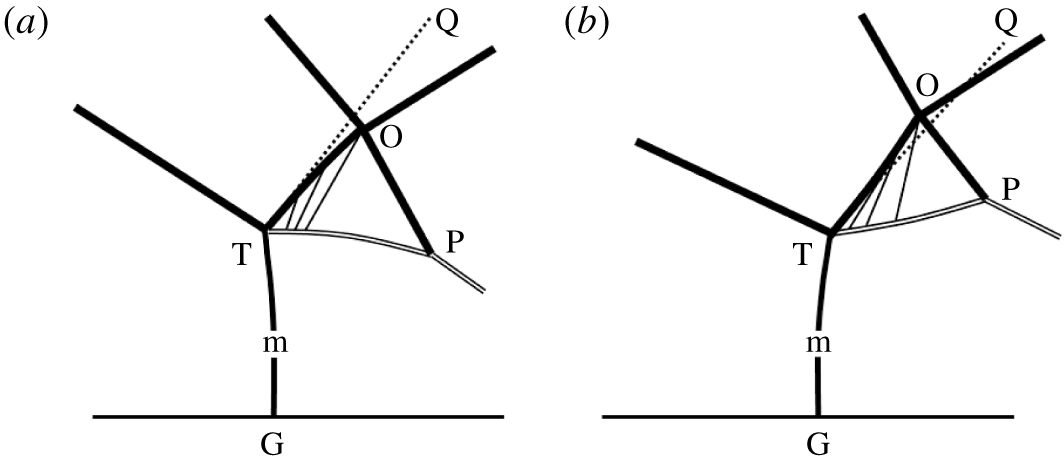
 $\unicode[STIX]{x1D6FD}_{2}^{(T)}$, meaning that the reflected shock wave deflects upward due to the secondary waves being compressive in the case of an inverted Mach stem, as shown schematically in figure 7(a). Table 1 also shows that
 $\unicode[STIX]{x1D6FF}_{sw}^{(N)}<\unicode[STIX]{x1D6FF}^{(N)}$ and
 $\unicode[STIX]{x1D6FF}_{sw}^{(D)}<\unicode[STIX]{x1D6FF}^{(D)}$, i.e. both the von Neumann condition and detachment condition are lowered by the shock strengthening effect of the compressive secondary waves. At least for the parameter range considered, the effect of the secondary waves is weak. For instance,
 $\unicode[STIX]{x1D6FD}_{2}^{(O)}$ is greater than
 $\unicode[STIX]{x1D6FD}_{2}^{(T)}$ by less than 0.3 degrees. At
 $\unicode[STIX]{x1D6FF}=13.75^{\circ }$,
 $\unicode[STIX]{x1D6FF}_{sw}^{(N)}=13.822^{\circ }$ compared to
 $\unicode[STIX]{x1D6FF}^{(N)}=13.918^{\circ }$ (
 $\unicode[STIX]{x1D6FF}_{sw}^{(N)}-\unicode[STIX]{x1D6FF}^{(N)}=-0.096^{\circ }$), and
 $\unicode[STIX]{x1D6FF}_{sw}^{(D)}=15.317^{\circ }$ compared to
 $\unicode[STIX]{x1D6FF}^{(D)}=15.418^{\circ }$ (
 $\unicode[STIX]{x1D6FF}_{sw}^{(D)}-\unicode[STIX]{x1D6FF}^{(D)}=-0.101^{\circ }$).
Influence of secondary waves on the reflected shock wave and transition criteria for inverted Mach stem case with  $M_{0}=3.98$ and
 $\unicode[STIX]{x1D703}_{w}=18^{\circ }$. In the present case,
 $\unicode[STIX]{x1D6FD}_{2}^{(T)}=44.597^{\circ }$,
 $\unicode[STIX]{x1D703}_{2}^{(T)}=-5.158^{\circ }$,
 $\unicode[STIX]{x1D6FF}^{(N)}=13.918^{\circ }$ and
 $\unicode[STIX]{x1D6FF}^{(D)}=15.418^{\circ }$.

Illustration of deflection of shock wave OT by secondary waves (the deflection is amplified in order to be clear). (a) Usual Mach reflection; (b) inverted Mach reflection.

For a usual Mach stem case, with  $M_{0}=3.98$ and
 $\unicode[STIX]{x1D703}_{w}=21.5^{\circ }$, the theoretical values of
 $\unicode[STIX]{x1D6FD}_{2}^{(O)}-\unicode[STIX]{x1D6FD}_{2}^{(T)}$,
 $\unicode[STIX]{x1D703}_{2}^{(O)}$,
 $\unicode[STIX]{x1D6FF}_{sw}^{(N)}$ and
 $\unicode[STIX]{x1D6FF}_{sw}^{(D)}$ with several
 $\unicode[STIX]{x1D6FF}$ close to the double solution domain are displayed in table 2. Contrary to the inverted Mach case, the shock angle
 $\unicode[STIX]{x1D6FD}_{2}^{(O)}$ is now smaller than
 $\unicode[STIX]{x1D6FD}_{2}^{(T)}$, meaning that the reflected shock wave deflects downward due to the secondary waves being expansive in the case of the usual Mach stem, as shown schematically in figure 7(b). Table 2 also shows that
 $\unicode[STIX]{x1D6FF}_{sw}^{(N)}>\unicode[STIX]{x1D6FF}^{(N)}$ and
 $\unicode[STIX]{x1D6FF}_{sw}^{(D)}>\unicode[STIX]{x1D6FF}^{(D)}$, i.e. both the von Neumann condition and detachment condition, are elevated by the shock weakening effect of the expansive secondary waves. The effect of secondary waves is much weaker than the last case. For instance,
 $\unicode[STIX]{x1D6FD}_{2}^{(O)}$ is smaller than
 $\unicode[STIX]{x1D6FD}_{2}^{(T)}$ by less than 0.05 degrees. The correction to
 $\unicode[STIX]{x1D6FF}^{(N)}$ and
 $\unicode[STIX]{x1D6FF}^{(D)}$ is also very small.
Influence of secondary waves on the reflected shock wave and transition criteria for the usual Mach stem case with  $M_{0}=3.98$ and
 $\unicode[STIX]{x1D703}_{w}=21.5^{\circ }$. For this case,
 $\unicode[STIX]{x1D6FD}_{2}^{(T)}=44.014^{\circ }$,
 $\unicode[STIX]{x1D703}_{2}^{(T)}=1.170^{\circ }$,
 $\unicode[STIX]{x1D6FF}^{(N)}=14.021^{\circ }$ and
 $\unicode[STIX]{x1D6FF}^{(D)}=14.473^{\circ }$.

To summarize, for inverted Mach reflection, which occurs when the first incident shock wave is below the usual von Neumann condition, the shock strengthening effect due to compressive Mach waves over the slipline TP lowers the double solution domain or advances the transition from type I shock interference to type II shock interference at point O. For usual Mach reflection, which occurs when the first incident shock wave is above the usual von Neumann condition, the shock weakening effect due to expansive Mach waves over the slipline TP elevates the double solution domain or delays the transition from type I shock interference to type II shock interference at point O.
Although the correction by secondary waves is apparently small, their effect can be observed in numerical simulation, as will be clear in § 4.2.
4 Numerical results displaying double solution and influence of secondary waves
The compressible Euler equations in gas dynamics are solved here, using the second-order Roe scheme. The same approach has been used by Lin, Bai & Wu (Reference Lin, Bai and Wu2019) for asymmetric shock reflection and verified using one experimental case of Li et al. (Reference Li, Chpoun and Ben-Dor1999). We use a grid with  $2000\times 400$ cells. This grid is much denser than that used by Guan et al. (Reference Guan, Bai and Wu2018) for shock reflection with two incident shock waves and as dense as that of Lin et al. (Reference Lin, Bai and Wu2019) for asymmetric shock reflection. The lengths of the wedge surfaces are chosen to be
 $w_{1}=1.1,w_{2}=0.2$ in all numerical computations. The inlet height
 $H_{A}$ is chosen to ensure that the two incident shock waves reflect at the same point on the reflecting surface in the case of normal reflection.
4.1 Numerical evidence of double solution
The purpose here is to look at whether a double solution can be observed numerically when the flow conditions are well inside the double solution domain predicted in § 2. For this purpose, we choose two cases, for which  $\unicode[STIX]{x1D6FF}$ lies well inside the double solution domain according to figure 3. For case 1, we set
 $M_{0}=3.98$,
 $\unicode[STIX]{x1D703}_{w}=18^{\circ }$,
 $\unicode[STIX]{x1D6FF}=14^{\circ }$. For case 2, we set
 $M_{0}=4.96$,
 $\unicode[STIX]{x1D703}_{w}=15^{\circ }$,
 $\unicode[STIX]{x1D6FF}=18^{\circ }$.
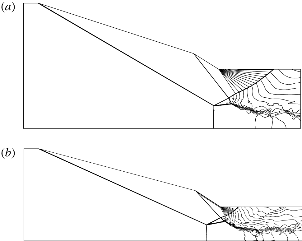
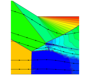
(i) Solution with type I shock interference. A uniform initial condition using the inlet condition as the initial condition is applied in the entire flow domain. For this computation, the Mach contours of two cases are displayed in figure 8(a,b), in which we see a type I shock interference at point O of figure 1.
Type I shock interference solutions. (a)  $M_{0}=3.98$,
 $\unicode[STIX]{x1D703}_{w}=18^{\circ },\unicode[STIX]{x1D6FF}=14^{\circ }$; (b)
 $M_{0}=4.96$,
 $\unicode[STIX]{x1D703}_{w}=15^{\circ },\unicode[STIX]{x1D6FF}=18^{\circ }$.

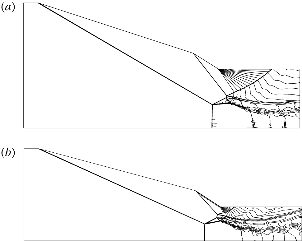
(ii) Solution with type II shock interference. We first compute a flow with inflow conditions chosen in the detachment region to obtain a solution with type II shock interference at point O. Then, we repeat the computation using this flow as the initial condition but setting the flow condition in the double solution domain. The Mach contours thus obtained for the two test cases are displayed in figure 9(a,b), in which we see a type II shock interference at point O of figure 1.
Type II shock interference solution. (a)  $M_{0}=3.98$,
 $\unicode[STIX]{x1D703}_{w}=18^{\circ }$ and
 $\unicode[STIX]{x1D6FF}=14^{\circ }$. (b)
 $M_{0}=4.96$,
 $\unicode[STIX]{x1D703}_{w}=15^{\circ }$ and
 $\unicode[STIX]{x1D6FF}=18^{\circ }$.

Thus, the existence of double solution predicted by transition criteria presented in § 2 is confirmed numerically using two Mach numbers, provided that the flow parameters are well inside the double solution domain.
4.2 Numerical verification of correction of secondary waves to transition criteria
First we consider  $M_{0}=3.98$,
 $\unicode[STIX]{x1D703}_{w}=18^{\circ }$ and
 $\unicode[STIX]{x1D6FF}=14.5^{\circ }$. According to the transition criteria displayed in figure 3,
 $\unicode[STIX]{x1D6FF}=14.5^{\circ }$ is close and below the detachment condition (
 $\unicode[STIX]{x1D6FF}^{(D)}=15.418^{\circ }$) so we should have a double solution. However, using the inlet condition as the initial condition as for the case of
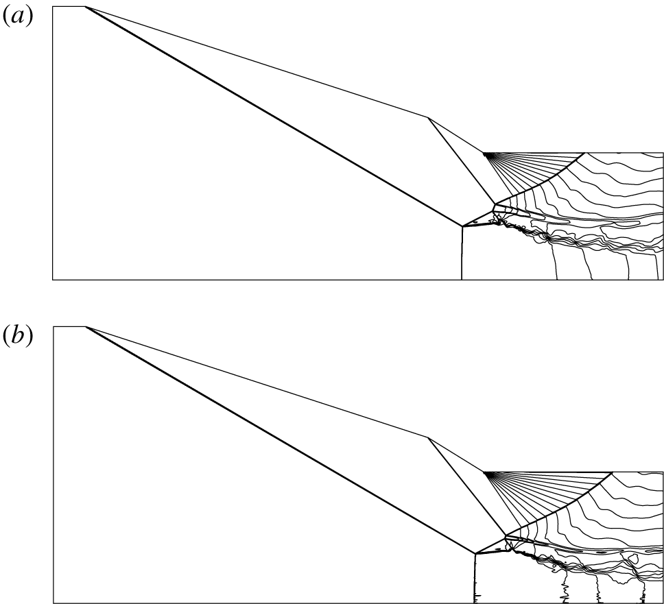
 $\unicode[STIX]{x1D6FF}=14^{\circ }$, we are unable to produce type I shock interference at point O and we only obtain type II shock interference, as is shown in figure 10(a) for the Mach contours.
Mach contours displaying variance of transition criteria for  $M_{0}=3.98$,
 $\unicode[STIX]{x1D703}_{w}=18^{\circ }$. (a) Double solution domain with
 $\unicode[STIX]{x1D6FF}=14.5^{\circ }$, displaying only type II shock interference. (b) The von Neumann solution domain with
 $\unicode[STIX]{x1D6FF}=13.75^{\circ }$, displaying type II shock interference.

Consider now  $M_{0}=3.98$,
 $\unicode[STIX]{x1D703}_{w}=18^{\circ }$ and
 $\unicode[STIX]{x1D6FF}=13.75^{\circ }$. According to the transition criteria displayed in figure 3,
 $\unicode[STIX]{x1D6FF}=13.75^{\circ }$ is close to but below the von Neumann condition (
 $\unicode[STIX]{x1D6FF}^{(N)}=13.918^{\circ }$) and should only yield a type I solution at point O. However, using the same method as for obtaining type II shock interference for case 1 of § 4.1 (
 $M_{0}=3.98$,
 $\unicode[STIX]{x1D703}_{w}=18^{\circ }$,
 $\unicode[STIX]{x1D6FF}=14^{\circ }$), we are able to produce a type II shock interference at point O, as shown in figure 10(b) for the Mach contours.
For  $M_{0}=3.98$,
 $\unicode[STIX]{x1D703}_{w}=18^{\circ }$ and
 $\unicode[STIX]{x1D6FF}=13.75^{\circ }$, we have
 $\unicode[STIX]{x1D6FF}_{sw}^{(N)}=13.822^{\circ }$ according to table 1. Thus,
 $\unicode[STIX]{x1D6FF}=13.75^{\circ }$ is even lower than the corrected von Neumann criterion
 $\unicode[STIX]{x1D6FF}_{sw}^{(N)}$. This means the theoretical values presented in table 1 are only approximate due to the necessary simplification adopted. Qualitatively, both theory and numerical experiment show that the double solution domain is lowered by the secondary waves.
4.3 Influence of transition on Mach stem heights
For  $M_{0}=3.98$,
 $\unicode[STIX]{x1D703}_{w}=18^{\circ }$ and for
 $\unicode[STIX]{x1D6FF}=12^{\circ }{-}15^{\circ }$, the numerical results for Mach stem heights
 $H_{T}$ and the lengths of shock
 $\text{O}_{1}\text{O}_{2}$ (denoted by
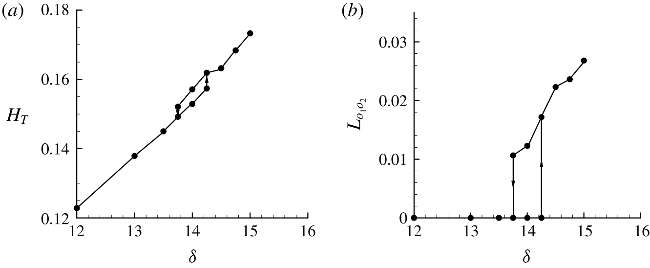
 $L_{o_{1}o_{2}}$) are shown in figure 11(a,b).
For  $13.75^{\circ }\leqslant \unicode[STIX]{x1D6FF}\leqslant 14.25^{\circ }$, we have two values of
 $H_{T}$ and
 $L_{o_{1}o_{2}}$, meaning hysteresis occurs across the double solution domain. It is clear that transition to type II shock interference at point O increases the Mach height
 $H_{T}$ for reason explained below.
The Mach heights  $H_{T}$ and the length of shock
 $\text{O}_{1}\text{O}_{2}$ (denoted by
 $L_{o_{1}o_{2}}$), with
 $M_{0}=3.98$,
 $\unicode[STIX]{x1D703}_{w}=18^{\circ }$ and
 $\unicode[STIX]{x1D6FF}=12^{\circ }{-}15^{\circ }$.

We have looked at the positions of the triple point T and the shock/slipline reflection point P with type I and type II shock interference at point O. Both T and P move upstream when shock interference at point O transits from type I to type II, as shown in table 3 for the particular case of  $\unicode[STIX]{x1D6FF}=14^{\circ }$. Since the triple point T is on the first incident shock wave, its shift to the upstream direction means increases of its vertical position, i.e. its height.
Numerical results for the positions of T and P, for  $M_{0}=3.98$,
 $\unicode[STIX]{x1D703}_{w}=18^{\circ }$,
 $\unicode[STIX]{x1D6FF}=14^{\circ }$.

4.4 Summary of the work and further questions
For pre-Mach reflection caused by two incident shock waves, the shock interference pattern at point O (intersection point of the reflected shock wave and the second incident shock wave) may be type I or type II. Transition criteria are obtained showing a double solution exists for a range of  $\unicode[STIX]{x1D6FF}$ at given
 $M_{0}$ and
 $\unicode[STIX]{x1D703}_{w}$. Numerical simulation shows that transition from type I to type II shock interference at point O increases the Mach stem height.
The transition from type I to type II shock interference is shown to be advanced by secondary waves generated over the slipline if the Mach stem is inverted. The transition from type I to type II shock interference is shown to be delayed by secondary waves generated over the slipline if the Mach stem is usual. This displays for the first time that the transition criterion may be modified by secondary Mach waves developed over the primary flow structure.
With curiosity, we wonder whether the effect of secondary waves may have an important effect on the Mach stem height even in the case of type I shock interference at point O. This is considered by introducing the correction of the shock angle at point O in the model of Guan et al. (Reference Guan, Bai and Wu2018). We observe that this correction does not have a noticeable effect on the Mach stem height. For instance, with  $M_{0}=3.98$,
 $\unicode[STIX]{x1D703}_{w}=23.5^{\circ }$ and
 $\unicode[STIX]{x1D6FF}=12^{\circ }$, we get
 $H_{T}=0.1866L$ (
 $L$ being the horizontal length of the wedge) using the original Mach stem height model of Guan et al. (Reference Guan, Bai and Wu2018) and we get
 $H_{T}=0.1880L$ if the correction of the reflected shock wave due to secondary waves is accounted for. For other conditions we draw a similar conclusion.
Secondary waves may also occur below or above the slipline(s) from the interaction point O. Secondary waves should also be generated there, curving further the slipline(s) and the shock waves beside the slipline(s). However, these secondary waves propagate in the downstream direction and have no intersection with the reflected shock wave (TO) and with the upstream part of the second incident shock wave (DO). As a result, the transition criteria are not subjected to the influence of these secondary waves.
As stated in the Introduction, we have ignored the real gas effect in this study.
We know that vibration energy is excited downstream of a normal shock wave if the upstream Mach number is greater than 3 and chemical reactions occur if the upstream Mach number is greater than 8 (Anderson Reference Anderson2019). Thus, the real gas effect should play a role for Mach numbers greater than 3. In this paper, although we have considered cases with a Mach number exceeding 3, we have omitted the influence of this effect. This real gas effect reduces the temperature and pressure downstream of shock waves. However, ignoring this effect does not alter the qualitative conclusions (existence of a double solution at point O and correction of the transition criteria by secondary waves) of the present paper since these conclusions hold in the case of small Mach number.
The effect of the viscosity is also omitted in this paper. For shock reflection with a single incident shock wave, Schmisseur & Gaitonde (Reference Schmisseur and Gaitonde2011) showed that no significant differences between inviscid and viscous calculations exist in the shear layers emanating from the triple point. This observation was further confirmed for Mach reflection with two incident shock waves by Guan et al. (Reference Guan, Bai and Wu2018). As pointed out by Schmisseur & Gaitonde (Reference Schmisseur and Gaitonde2011), the displacement effect of the wedge boundary layer increases the equivalent wedge angle and thus the incident shock angle. Thus, the conclusion based on an inviscid analysis can be used to understand similar phenomena in the viscous problem with a boundary layer, if we replace the wedge angle by the equivalent wedge angle due to the displacement effect. This is in fact demonstrated by Chen, Bai & Wu (Reference Chen, Bai and Wu2019) in the case of a single incident shock wave.
Another way to account for the influence of the boundary layer is to use a shock angle, instead of a wedge angle, as input since the boundary layer displacement effect is implicitly accounted for in the shock angle. For instance, in studying Mach stem height, Hornung & Robinson (Reference Hornung and Robinson1982) and Li & Ben-Dor (Reference Li and Ben-Dor1997) used the shock angle as input.
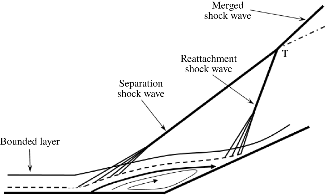
The situation is however more complex in case separation occurs at the wedge turning point.
As shown in figure 12 for the shock boundary layer interaction problem, the effects of viscosity may induce flow separation and complex compressive waves at the wedge deflection point. These compressive waves also merge into a single shock wave called the separation shock wave. Another shock wave is the reattachment shock wave. If a reflecting surface is put at a point sufficiently far away from the corner, then the separation shock wave and reattachment shock wave may have merged into a single incident shock wave. If the reflecting surface is placed at the point (point T) where the separation and reattachment shock waves just intersect, then we have a local problem that can be considered as the reflection of two incident shock waves.
Adding real gas effects to the theoretical models in §§ 2 and 3 would make the theory very complex or intractable. Ignoring these effects in the present study allows us to focus on inviscid phenomena and understand the influence of the transition at point O and secondary waves. A quantitative study of such a problem taking into account all the complex effects should rely on computational fluid dynamics.
The shock wave boundary layer interaction phenomena ahead of a compression corner (figure produced following figure 1(a) of Verma, Manisankar & Akshara (Reference Verma, Manisankar and Akshara2015)).

Acknowledgements
The referees and associate editor provided us with many valuable suggestions leading to great improvement of the paper. This work was supported by the Natural National Science Foundation of China (no. 11802157).
Declaration of interests
The authors report no conflict of interest.