
I. INTRODUCTION
The hot deformation of metals or alloys is a comprehensive process under the influences of temperature, strain rate, and microstructure evolution. It is difficult to make efficient quantitative analysis on hot deformation behavior of materials by experimental methods. With the development of numerical simulation techniques, a numerical simulation is widely applied to analyse the manufacturing processes of materials and are used to study the forming mechanism and further optimize the product design. Constitutive equation is the mathematical representation of the flow behavior of materials during simulation under the loading conditions. Reference Lin, Nong, Chen, Chen and Chen1 Consequently, describing the deformation behavior of materials accurately by the constitutive equations is the key to achieve high accuracy of numerical simulation result. Reference Chen, Lin, Zhou, Chen and Wen2
Several models, such as empirical, phenomenological, and physical-based constitutive models, have been proposed to describe the flow stress characteristics of metals and alloys. Among of these models, the JC model Reference Johnson and Cook3 is an empirical constitutive model, which has been widely used for different metallic materials at a large deformation with high strain rates and temperature, such as aluminum alloys, Reference Lin, Li, Xia and Li4–Reference Zhang, Shangguan, Xie and Liu6 titanium alloys, Reference Buzyurkin, Gladky and Kraus7,Reference Kotkunde, Deole, Gupta and Singh8 and steels. Reference Lin and Chen9–Reference Gambirasio and Rizzi11 However, most constitutive models coincide well with actual results only at the small strain stage.
To predict more accurately for the whole deformation process, some mathematical models are developed. Considering the interactions between deformation temperature and strain rate, the Arrhenius-type constitutive model was developed, which extensively used to represent the relationship among the flow stress, temperature, and strain rate. Reference Rokni, Zarei-Hanzaki, Roostaei and Abolhasani12,Reference Chen, Zhao, Yu and Zhang13 In recent years, some researchers found that strain has an influence on the material parameters, then the strain-compensated Arrhenius model was established, Reference Wang, Zhao, Chen and Li14–Reference Chen, Zhao and Yu16 and the prediction accuracy was improved.
Besides, researchers also pay attention to the physical essence of materials during the hot deformation. Based on the dislocation density evolution which characterizes the physical mechanism of work hardening (WH), dynamic recovery (DRV), and dynamic recrystallization (DRX), a physically based constitutive model was established to describe the flow stress of materials. Reference Lin, Chen and Zhong17,Reference Ji, Li, Ding, Yang and Li18 The physically based constitutive models can explain physical mechanisms of deformation under a certain condition and predict experimental results accurately. As a result, it has been developed to predict the flow stress of superalloys, Reference Zhang, Yi, Chen, Qin and Wang19 Cu alloys, Reference Ji, Li, Ding, Yang and Li18,Reference Ji, Li and Li20 and steels. Reference Shen, Zhang, Zhang, Xu and Shi21,Reference He, Xie, Yang, Wang and Zhang22 In view of these constitutive equations, some studies were performed on comparing the different constitutive models for metallic materials to evaluate the applicability. Reference Samantaray, Mandal and Bhaduri23–Reference He, Xie, Zhang and Wang25
34CrNiMo-alloyed steel is a representative kind of medium carbon Cr–Ni–Mo-alloyed steel with superior mechanical properties, which is widely used for manufacturing crankshafts, wind turbines, and other high quality forging units. During the hot deformation processes of materials, such as forging and rolling, it is important to control the mechanical performance of the final product. To obtain high quality products, it is necessary to study the flow behavior of materials in detail. For the medium carbon Cr–Ni–Mo-alloyed steel, most previous studies investigated the recrystallization behaviors during hot deformation. Reference Zhang, Zhang, Xu, Xia and Shen26,Reference Kuduzovic, Poletti, Sommitsch, Domankova, Mitsche and Kienreich27 Less attention has been paid to modeling the flow behavior of this kind of medium carbon Cr–Ni–Mo-alloyed steel. Besides, some constitutive equations were tried to be established to model the flow behavior of medium carbon steel. Reference Meysami and Mousavi28,Reference Lin, Chen and Zhang29 However, few systematic researches about the comparisons among different constitutive models of the flow stress behavior of medium carbon steel have been reported.
In this work, the JC model, Arrhenius-type constitutive model, and physically based constitutive model were developed to describe the flow behavior of 34CrNiMo steel during the hot compression procedure. The flow stresses predicted by the developed constitutive equations were compared with the experimental ones, respectively. Moreover, the accuracy and efficiency of these models were compared according to the statistical analysis of the predicted values.
II. MATERIAL AND EXPERIMENT
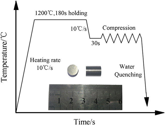
The chemical composition of the 34CrNiMo steel used in the test is shown in Table I. The billets were machined into cylindrical specimens with a diameter of 8 mm and a height of 12 mm. The hot compression tests were performed using a Gleeble-1500 thermal mechanical simulator (Dynamic Systems Inc., Poestenkill, New York). All of the specimens were heated to 1473 K at a rate of 10 K/s and were held for 180 s to acquire a homogeneous and equiaxed microstructure. Then, the specimens were cooled to 1173, 1223, 1273, 1323, 1373, and 1423 K, respectively, with a rate of 10 K/s and held for 30 s to eliminate the temperature gradient before the compression. After that, the compressions were performed under the strain rates of 0.002, 0.01, 0.1, 1, and 5 s−1. At the end of deformation, the specimens were quenched in water immediately. Figure 1 illustrates the schematic diagram and the specimen of the hot compression process.
Chemical composition of the tested steel (wt%).

The experimental procedure and the specimen of hot the compression test.

III. RESULTS AND DISCUSSION
A. Flow stress behavior
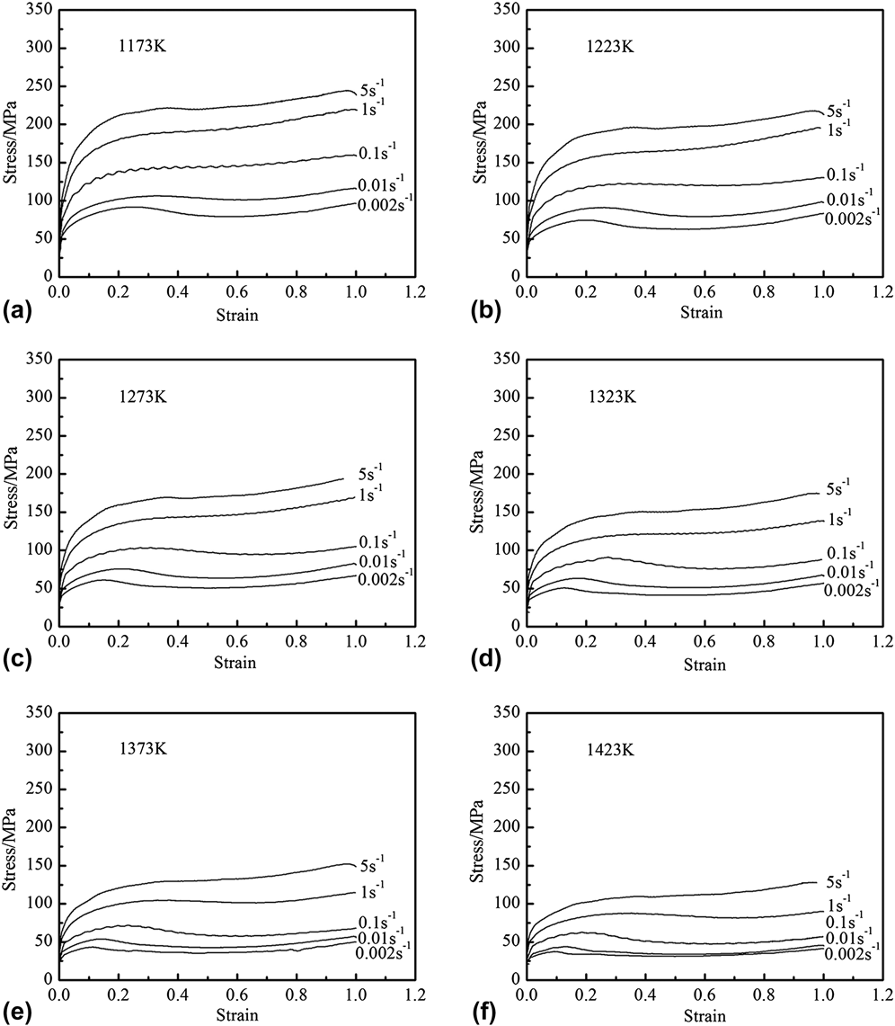
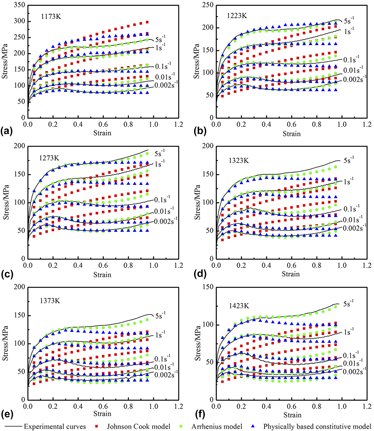
The stress–strain curves of 34CrNiMo alloyed steel obtained from hot compression tests are shown in Fig. 2. It can be seen that the deformation temperature and strain rate have great influences on flow stress. The flow stress decreases with the increasing temperature and the decreasing strain rate under the same strain condition. Besides, the flow stresses have typical recovery and recrystallization characteristics. At the initial stage of the deformation process, the stress increases to a peak value because the WH has an advantage over the DRV. The dislocation density increases dramatically in this stage to preserve the deformation energy. Reference Liu, Lin and Zhou30 When the deformation exceeds the peak strain (εp), the flow stress declines gradually to the steady value with the continuous increasing strain. This softening is caused by the nucleation and growth of DRX grains with a rather low dislocation density. Reference Shen, Zhang, Zhang, Xu and Shi21,Reference Wen, Lin and Zhou31
Stress–strain curves of 34CrNiMo steel with various deformation temperatures under the temperatures of (a) 1173 K, (b) 1223 K, (c) 1273 K, (d) 1323 K, (e) 1373 K, and (f) 1423 K.

B. Johnson Cook model
The JC constitutive model describes the stress–strain relationship in metallic materials during hot deformation, and the flow stress is expressed as follows. Reference Johnson and Cook3
 $$\sigma = \left( {A + B{\varepsilon ^n}} \right)\left( {1 + C\ln {{\dot \varepsilon }^ * }} \right)\left( {1 - {T^{ * m}}} \right)\quad ,$$
where σ is the equivalent flow stress (true stress), ε is the equivalent plastic strain (true strain), A is the yield stress of the material at the condition of reference temperature and reference strain rate, B is the coefficient of strain hardening, n is the strain-hardening exponent, C and m are the material constants, which represent the coefficient of strain rate hardening and thermal softening exponent, respectively.
 ${\dot \varepsilon ^ * } = \dot \varepsilon /{\dot \varepsilon _{\rm{r}}}$
is the dimensionless strain rate (which
 $\dot \varepsilon$
is the strain rate, while
 ${\dot \varepsilon _{\rm{r}}}$
is the reference strain rate) and
 ${T^ * }$
is the homologous temperature and is expressed as follows.
 $${T^ * } = {{T - {T_{\rm{r}}}} \over {{T_{\rm{m}}} - {T_{\rm{r}}}}}\quad ,$$
where T is the current absolute temperature, T m is the melting temperature, and T r is the reference temperature (T ≥ T r), all of which should be absolute temperature (K).
In this study, the reference temperature and strain rate were selected as T
r = 1173 K and
 ${\dot \varepsilon _{\rm{r}}} = 0.002\;{{\rm{s}}^{ - 1}}$
, respectively. The value of A was determined as the yield stress, where A = 40.796 MPa.
At the reference temperature and strain rate, the flow stress could be expressed as follows.
 $$\sigma = A + B{\varepsilon ^n}\quad .$$
Substituting the value of A in Eq. (1) and using the flow stress data at various strains under reference conditions, the relationship between ln(σ − A) and ln ε could be obtained, as shown in Fig. 3. The value of n could be calculated from the slope of the fitting line while ln B is obtained from the intercept of the line.
Relationship between ln(σ − A) and ln ε at a temperature of 1173 K and a strain rate of 0.002 s−1.

At the reference temperature, Eq. (1) could be expressed as:
 $${\sigma \over {A + B{\varepsilon ^n}}} = 1 + C\ln {\dot \varepsilon ^ * }\quad .$$
Figure 4 shows the relationship between σ/(A + Bε
n
) and
 $\ln {\dot \varepsilon ^ * }$
. Then, C can be obtained as the slope.
Relationship between σ/(A + Bε
n
) and
 $\ln {\dot \varepsilon ^ * }$
.

Similarly, at the reference strain rate, the flow stress data in different temperatures would be independent from the thermal softening term, thus Eq. (1) could be expressed as:
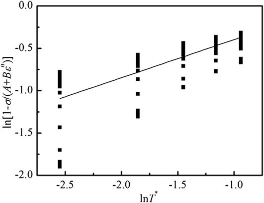
 $${\sigma \over {A + B{\varepsilon ^n}}} = 1 - {T^{ * m}}\quad .$$
Figure 5 shows the relationship between ln[1 − σ/(A + Bε n )] and ln T*, the constant m could be obtained from the slope of this fitting line.
Relationship between ln[1 − σ/(A + Bε n )] and ln T*.

Finally, the JC model of 34CrNiMo steel could be described as follows.
 $$\sigma = \left( {40.796 + 90.810{\varepsilon ^{0.367}}} \right)<$$><$$>\left( {1 + 0.165\ln {{\dot \varepsilon }^ * }} \right)\left( {1 - {T^{ * 0.450}}} \right)\quad .$$
C. Strain compensated arrhenius model
The relationship among the flow stress, strain rate, and temperature could be described by the Arrhenius equation. The effects of the temperature and strain rate on deformation behavior can be represented by the Zener–Hollomon parameter in the form of an exponential equation. Reference Zener and Hollomon32 This could be mathematically expressed as:
 $$Z = \dot \varepsilon \exp \left( {{Q \over {RT}}} \right)\quad ,$$
in which,
 $\dot \varepsilon$
is the strain rate (s−1), R is the universal gas constant [8.314 J/(mol K)], and T is the absolute temperature (K). The Arrhenius model could be expressed as:
 $$\dot \varepsilon = AF\left( \sigma \right)\exp \left( {{{ - Q} \over {RT}}} \right)\quad ,$$
where
 $$F\left( \sigma \right) = \left\{ {\matrix{ {{\sigma ^{{n_1}}}} \hfill {\alpha \sigma \lt 0.8} \hfill \cr {\exp \left( {\beta \sigma } \right)} \hfill {\alpha \sigma \ge 1.2} \hfill \cr {{{\left[ {\sinh \left( {\alpha \sigma } \right)} \right]}^n}} \hfill {{\rm{for}}\;{\rm{all}}\;\sigma } \hfill \cr} } \right.\quad ,$$
where, σ is the flow stress (MPa) for a given strain, A, α, and n are the material constants, α = β/n 1.
For low and high stress levels, Eq. (8) could be repressed as Reference Sellars and McTegart33,Reference Jonas, Sellars and Tegart34 :
 $$\dot \varepsilon = A{\left[ {\sinh \left( {\alpha \sigma } \right)} \right]^n}\exp \left( {{{ - Q} \over {RT}}} \right)\quad .$$
To derive the required material constants and further to establish the Arrhenius model of 34CrNiMo steel, the natural logarithm of Eq. (10) is taken, the following equation can be obtained.
 $$\ln \dot \varepsilon = \ln A + n\ln \left[ {\sinh \left( {\alpha \sigma } \right)} \right] - {Q \over {RT}}\quad .$$
For a particular deformation temperature and strain rate condition, by differentiating Eq. (11), the following formula could be derived, respectively:
 $$n = {\left\{ {{{\partial \ln \dot \varepsilon } \over {\partial \ln \left[ {\sinh \left( {\alpha \sigma } \right)} \right]}}} \right\}_T}\quad .$$
 $$Q = Rn{\left\{ {{{\partial \ln \left[ {\sinh \left( {\alpha \sigma } \right)} \right]} \over {\partial \left( {{1 \mathord{\left/ {\vphantom {1 T}} \right. \kern-\nulldelimiterspace} T}} \right)}}} \right\}_{\dot \varepsilon }}\quad .$$
The values of material constants of A could be obtained by taking the natural logarithm on both sides of Eq. (10), which is expressed as:
 $$\ln Z = \ln A + n\ln \left[ {\sinh \left( {\alpha \sigma } \right)} \right]\quad .$$
Then the flow stress could be written as a function of the Z parameter as:
 $$\sigma = {1 \over \alpha }\ln \left\{ {{{\left( {{Z \over A}} \right)}^{{1 \mathord{\left/ {\vphantom {1 n}} \right. \kern-\nulldelimiterspace} n}}} + {{\left[ {{{\left( {{Z \over A}} \right)}^{{2 \mathord{\left/ {\vphantom {2 n}} \right. \kern-\nulldelimiterspace} n}}} + 1} \right]}^{{1 \mathord{\left/ {\vphantom {1 2}} \right. \kern-\nulldelimiterspace} 2}}}} \right\}\quad .$$
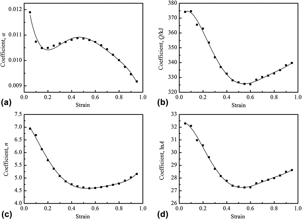
In this study, the values of material constants of the Arrhenius model were calculated under different strains in the practical range of 0.05–0.95 with an interval of 0.05 using the same method. Figure 6 shows the influences of strain on material constants at the entire strain range. And a fifth order polynomial fitting Reference Mandal, Rakesh, Sivaprasad, Venugopal and Kasiviswanathan35 can be used to describe the relationship between the strain and the material constants of α, Q, n, and ln A, as given by Eq. (16).
 $$\left\{ \matrix{ \alpha \left( \varepsilon \right) = {\alpha _0} + {\alpha _1}\varepsilon + {\alpha _2}{\varepsilon ^2} + {\alpha _3}{\varepsilon ^3} + {\alpha _4}{\varepsilon ^4} + {\alpha _5}{\varepsilon ^5} \hfill \cr Q\left( \varepsilon \right) = {Q_0} + {Q_1}\varepsilon + {Q_2}{\varepsilon ^2} + {Q_3}{\varepsilon ^3} + {Q_4}{\varepsilon ^4} + {Q_5}{\varepsilon ^5} \hfill \cr n\left( \varepsilon \right) = {n_0} + {n_1}\varepsilon + {n_2}{\varepsilon ^2} + {n_3}{\varepsilon ^3} + {n_4}{\varepsilon ^4} + {n_5}{\varepsilon ^5} \hfill \cr \ln A\left( \varepsilon \right) = {A_0} + {A_1}\varepsilon + {A_2}{\varepsilon ^2} + {A_3}{\varepsilon ^3} + {A_4}{\varepsilon ^4} + {A_5}{\varepsilon ^5} \hfill \cr} \right.\quad .$$
Relationships between material constants and true strain on the material constants fit by fifth order polynomial: (a) α, (b) Q, (c) n, and (d) ln A.

The coefficients of the above polynomial functions are given in Table II. Furthermore, the flow stress can be described by strain, stain rate, and deformation temperature according to Eq. (15) with the Arrhenius model.
Coefficients of the polynomial functions.

D. Physically based constitutive model
When the strain is below the critical strain (εc), the DRX does not occur. Reference Mecking and Kocks36 The evolution of dislocation density (ρ) for metals during this stage is supposed to be determined by the coupled effects of generation by WH and annihilation by DRV. The dependence of the dislocation density on strain can be written as follows.
 $${{{\rm{d}}\rho } \over {{\rm{d}}\varepsilon }} = U - \Omega \rho \quad ,$$
where dρ/dε is the rate of increase of the dislocation density with strain, U is the WH rate, and Ω is noted as the coefficient of dynamic recovery. By integrating Eq. (17), it gives:
 $$\rho = \exp \left( { - \Omega \varepsilon } \right)\left[ {{U \mathord{\left/ {\vphantom {U {\Omega \exp \left( { - \Omega \varepsilon } \right)}}} \right. \kern-\nulldelimiterspace} {\Omega \exp \left( { - \Omega \varepsilon } \right)}} + {\rho _0} - {U \mathord{\left/ {\vphantom {U \Omega }} \right. \kern-\nulldelimiterspace} \Omega }} \right]\quad ,$$
where ρ0 is the initial dislocation density (when ε = 0). At the condition of high temperatures, the effective stress can be neglected compared to the internal stress, then the applied stress is related to the dislocation density as:
 $\sigma = \alpha \mu b\sqrt \rho$
, where α is constant for a given material, μ is the shear modulus, and b is the magnitude of the Burger’s vector.
Reference Laasraoui and Jonas37,Reference Jorge Junior and Balancin38
Therefore, the flow stress during WH and DRV periods can be expressed as a function of strain by combining the above equations.
 $$\sigma = {\left[ {\sigma _{{\rm{sat}}}^2 + \left( {\sigma _0^2 - \sigma _{{\rm{sat}}}^2} \right)\exp \left( { - \Omega \varepsilon } \right)} \right]^{0.5}}\quad \left( {\varepsilon \lt {\varepsilon _{\rm{c}}}} \right)\quad ,$$
where σsat is the saturation stress and σ0 is the initial stress.
In the DRX region, the evolution of dislocation density depends on the DRX kinetics. The Avrami equation can be used to describe the kinetics of the DRX behavior as follows. Reference Jonas, Quelennec, Jiang and Martin39
 $${X_{\rm{d}}} = 1 - \exp \left[ { - K{{\left( {{{\varepsilon - {\varepsilon _{\rm{c}}}} \over {{\varepsilon _{\rm{p}}}}}} \right)}^N}} \right]\quad ,$$
where N is the Avrami’s power, K is a constant, and εp is the peak strain corresponding to the peak stress.
Simultaneously, the DRX fraction can be evaluated by the decreasing of the flow stress.
 $${X_{\rm{d}}} = {{{\sigma _{\rm{p}}} - \sigma } \over {{\sigma _{\rm{p}}} - {\sigma _{{\rm{ss}}}}}}\quad ,$$
where σp and σss is the peak stress and steady state stress. Then the flow stress during the DRX region can be expressed as follows:
 $$\sigma = {\sigma _{\rm{p}}} - \left( {{\sigma _{\rm{p}}} - {\sigma _{{\rm{ss}}}}} \right)\left\{ {1 - \exp \left[ { - K{{\left( {{{\varepsilon - {\varepsilon _{\rm{c}}}} \over {{\varepsilon _{\rm{p}}}}}} \right)}^N}} \right]} \right\}\quad \left( {\varepsilon \ge {\varepsilon _{\rm{c}}}} \right)\quad .$$
According to the above analysis and methods, the physically based constitutive model for the flow stress of 34CrNiMo steel under hot deformation can be described by the following equations Reference Zhang, Zhang, Shen, Liu, Xia and Li40 :
 $$\left\{ {\matrix{ {\sigma = {{\left[ {\sigma _{{\rm{sat}}}^2 + \left( {\sigma _0^2 - \sigma _{{\rm{sat}}}^2} \right)\exp \left( { - \Omega \varepsilon } \right)} \right]}^{0.5}}} \hfill {\left( {\varepsilon \lt {\varepsilon _{\rm{c}}}} \right)} \hfill \cr {\sigma = {\sigma _{\rm{p}}} - \left( {{\sigma _{\rm{p}}} - {\sigma _{{\rm{ss}}}}} \right)\left\{ {1 - \exp \left[ { - K{{\left( {{{\varepsilon - {\varepsilon _{\rm{c}}}} \over {{\varepsilon _{\rm{p}}}}}} \right)}^N}} \right]} \right\}} \hfill {\left( {\varepsilon \ge {\varepsilon _{\rm{c}}}} \right)} \hfill \cr {Z = \dot \varepsilon \exp \left( {{{347000} \mathord{\left/ {\vphantom {{347000} {RT}}} \right. \kern-\nulldelimiterspace} {RT}}} \right)} \hfill {} \hfill \cr {\Omega = 49.550{Z^{ - 0.051}}} \hfill {{\varepsilon _{\rm{c}}} = 0.030{Z^{0.0521}}} \hfill \cr {{\sigma _{{\rm{sat}}}} = {\sigma _{\rm{p}}} = 1.777{Z^{0.133}}} \hfill {{\varepsilon _{\rm{p}}} = 0.009{Z^{0.112}}} \hfill \cr {{\sigma _{{\rm{ss}}}} = 0.799{Z^{0.156}}} \hfill {{\sigma _0} = 3.7336{Z^{0.091}}} \hfill \cr {K = 0.695} \hfill {N = 1.897} \hfill \cr} } \right.\quad .$$
E. Comparisons of constitutive equations
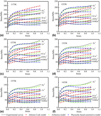
The comparisons between the experimental flow stress data and predicted data by the JC model, strain compensated Arrhenius model, and physically based constitutive model are shown in Fig. 7.
Comparison between the experimental data and predicted data by three models under the temperatures of (a) 1173 K, (b) 1223 K, (c) 1273 K, (d) 1323 K, (e) 1373 K, and (f) 1423 K.

To compare the accuracy of the JC model, strain-compensated Arrhenius model, and physically based constitutive model, the correlation coefficient (R) and the average absolute relative error (AARE) are used to evaluate the deviation between predicted flow stresses and experimental ones. The correlation coefficient (R) presents the power of linear relationship between the experimental and predicted values. AARE is a universal statistical parameter for representing the predictability of models. The calculations of statistical parameters are expressed as follows.
 $$R = {{\sum\limits_{i = 1}^{i = N} {\left( {\sigma _{\exp }^i - {{\bar \sigma }_{\exp }}} \right)\left( {\sigma _{{\rm{pre}}}^i - {{\bar \sigma }_{{\rm{pre}}}}} \right)} } \over {\sqrt {\sum\limits_{i = 1}^{i = N} {{{\left( {\sigma _{\exp }^i - {{\bar \sigma }_{\exp }}} \right)}^2}} \sum\limits_{i = 1}^{i = N} {{{\left( {\sigma _{{\rm{pre}}}^i - {{\bar \sigma }_{{\rm{pre}}}}} \right)}^2}} } }}\quad .$$
 $${\rm{AARE}}\left( \% \right) = {1 \over N}\sum\limits_{i = 1}^{i = N} {\left| {{{\sigma _{\exp }^i - \sigma _{{\rm{pre}}}^i} \over {\sigma _{\exp }^i}}} \right|} \times 100\% \quad ,$$
where N is the number of statistic data and i is the numbering of each value.
 $\sigma _{\exp }^i$
and
 $\sigma _{{\rm{pre}}}^i$
are the experimental flow stress and predicted flow stress calculated by constitutive models, respectively.
 ${\bar \sigma _{\exp }}$
and
 ${\bar \sigma _{{\rm{pre}}}}$
are the average values of the experimental flow stress and predicted flow stress calculated by constitutive models, respectively.
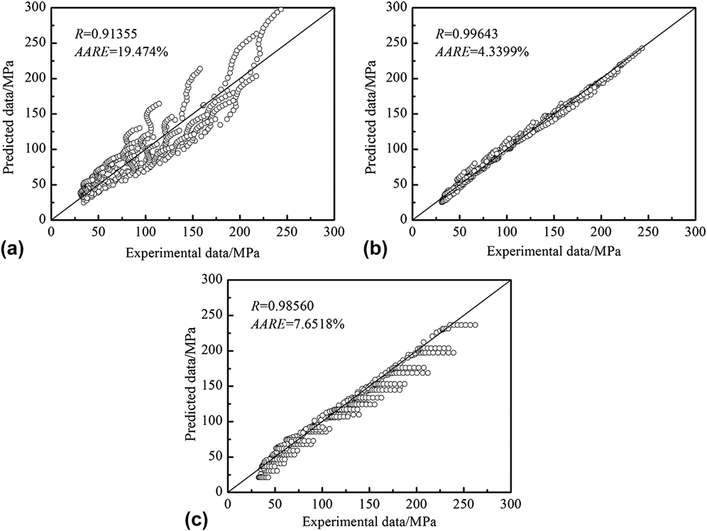
Figure 8 shows the correlations between the experimental and predicted flow stress data from three different constitutive models. The correlation coefficients for the JC model, strain compensated Arrhenius model, and physically based constitutive model are 0.914, 0.996, and 0.986, respectively. The AAREs are 19.47%, 4.34%, and 7.65%, respectively.
Comparisons between experimental and predicted data by three models: (a) Johnson Cook model, (b) Arrhenius model, and (c) considering DRV and DRX constitutive model.

From the comparison of statistical analysis, it is obvious that the JC model is not able to represent the high-temperature flow behavior of 34CrNiMo steel. The prediction values coincide with the experimental data only under a small range of strain when the WH is the prime deformation mechanism. It is because the JC model assumes that thermal softening, strain rate hardening, and strain hardening are three independent phenomena, which are isolated from each other. Reference Samantaray, Mandal and Bhaduri23 Due to the effects of recovery and recrystallization softening, the predicted data are greater than the experimental data, and the softening stage in the flow stress is not fit well using this model. Previous researches showed that the JC model can give an accurate description on the flow stress of materials which have typical WH or thermal softening behaviors individually, Reference Lin, Li, Fu and Jiang41,Reference Lin, Li and Jiang42 but it cannot describe these behaviors at the same time. Reference Abbasi-Bani, Zarei-Hanzaki, Pishbin and Haghdadi24
Considering the comprehensive influences of the strain rate and deformation temperature on the flow behavior, the strain compensated Arrhenius model has a higher accuracy to predict the flow stress under the entire processing conditions. Whereas, it only gives formula derivation in mathematics but has few interpretations in physics for the flow behavior during hot deformation processes.
The physically based constitutive model has a similar prediction accuracy to the Arrhenius-type model in terms of the correlation coefficient and AARE. Besides, it has considered the recovery and recrystallization procedure during the hot working and has a good agreement with the flow stress during the softening stage. Reference Zhang, Zhang, Shen, Liu, Xia and Li40 It indicates that the physically based constitutive model is capable of describing the flow stress behavior of the tested steel during hot deformation. Reference Shen, Zhang, Zhang, Xu and Shi21,Reference He, Xie, Yang, Wang and Zhang22,Reference Abbasi and Shokuhfar43 The predicted data using this model are less than the experimental ones at the end stage of deformation in most conditions. That is because that the lateral flow of the material is suppressed by friction, and the resistant stress of deformation is larger than the ideal condition, especially becomes more obvious at larger strains. Reference Ebrahimi and Najafizadeh44
IV. CONCLUSIONS
The 34CrNiMo steel, as a kind of medium carbon Cr–Ni–Mo alloyed steel, was chosen as the tested steel to study the flow stress behavior under elevated temperature. The hot compression tests were performed in a temperature range of 1173–1423 K and a strain rate range of 0.002–5 s−1. Based on the experimental data, a comparative study has been established to predict the flow stress behavior using the JC model, strain compensated Arrhenius model, and the physically based constitutive model. The main conclusions are summarized as follows.
-
(1) The flow stress behavior of 34CrNiMo steel has a typical recovery and recrystallization characteristic according to the strain–stress curves, deformation temperature and strain rate have noticeable influences on the flow stress.
-
(2) The JC model is not able to adequately represent the high temperature flow behavior of the 34CrNiMo steel, especially during the softening stage arising from recovery and recrystallization.
-
(3) The strain-compensated Arrhenius model has a higher accuracy in pure mathematics to predict the flow stress under the entire processing conditions, considering the influences of temperature and strain rate.
-
(4) The physically based constitutive model has a similar prediction accuracy with the experimental results. What is more, it considers the effects of recovery and recrystallization procedure during the hot working and gives good agreement with the flow stress in the softening stage caused by recovery and recrystallization.
ACKNOWLEDGMENTS
This work was supported by the National Natural Science Foundation of China (No. 51604058) and the Fundamental Research Funds for the Central Universities of China.