1. Introduction
A flexible foil immersed in a fluid flow experiences a self-induced self-sustained periodical flapping motion at sufficiently high flow speed. The flapping of elastic foil problem is of interest not only due to its prevalence, but also due to the simplicity of the problem statement and the richness of the coupled fluid–structure behaviour. The fluid-elastic instability with such a configuration can be easily seen by blowing air over a thin piece of paper or a leaf and in waving of flag-like structures. A flexible foil clamped at the leading edge and with the trailing edge free to oscillate, from here on referred to as a conventional foil, is stabilized by the viscous drag and structural stiffness, while the pressure force tends to produce the opposite effect. Applications of this phenomenon include the implementation of new surgical methods (Huang Reference Huang1995), increasing the speed of paper printing (Watanabe et al. Reference Watanabe, Isogai, Suzuki and Sugihara2002a ,Reference Watanabe, Suzuki, Sugihara and Sueoka b ), nuclear plate assemblies (Guo & Paidoussis Reference Guo and Paidoussis2000), flow control devices (Lucey Reference Lucey1998; Jaiman, Loth & Dutton Reference Jaiman, Loth and Dutton2004) and botanical applications (Huang, Rominger & Nepf Reference Huang, Rominger and Nepf2011). A system of flexible foils has been also proposed as a means of harvesting energy, which can be utilized to generate electric energy (Allen & Smits Reference Allen and Smits2001; Tang, Paidoussis & Jiang Reference Tang, Paidoussis and Jiang2009). In this view, Michelin & Doare (Reference Michelin and Doare2013) recently proposed a theoretical framework to study the optimal position of piezoelectric patches on an elastic foil to maximize the efficiency.
The flapping of a conventional flexible foil has been extensively studied using various theoretical, experimental and numerical methods. Paidoussis (Reference Paidoussis2000) and Shelley & Zhang (Reference Shelley and Zhang2011) have provided an extensive literature review on this topic. Early studies on the flapping instability (Dowell Reference Dowell1966, Reference Dowell1970) were based on linear instability analysis using the Galerkin decomposition in space to predict the critical velocity above which the flexible foil exhibits flapping motion. These studies largely focused on supersonic flow and were motivated by aerospace applications. Kornecki, Dowell & O’Brien (Reference Kornecki, Dowell and O’Brien1976) have theoretically investigated the flapping instability for subsonic flows by introducing a circulatory fluid loading to satisfy the Kutta condition at the trailing edge. Extending this theoretical analysis, Argentina & Mahadevan (Reference Argentina and Mahadevan2004) included the effects of viscous drag induced tension and finite size in their theoretical model. To analyse the influence of trailing and leading edge boundary conditions on the flapping instability, Guo & Paidoussis (Reference Guo and Paidoussis2000) performed a linear stability analysis in Fourier space.
More recently, Shelley, Vandenberghe & Zhang (Reference Shelley, Vandenberghe and Zhang2005), with the aid of a simplified analytical model and water-tunnel experiments, have shown that a flexible foil in a heavy fluid can experience strong added-mass effects, which can stabilize the foil. By employing a three-dimensional potential flow with two-dimensional foil deflections, Eloy, Souilliez & Schouveiler (Reference Eloy, Souilliez and Schouveiler2007) studied the effects of aspect ratio on the stability and dynamics of a flexible foil. In this study, the authors observed that flexible foils with small aspect ratios tend to be more stable compared with foils with larger aspect ratios. Eloy, Kofman & Schouveiler (Reference Eloy, Kofman and Schouveiler2012) further analysed the hysteresis effects observed experimentally and attributed these effects to the surface defects of the flexible plate. In addition to linear/nonlinear stability analyses, Tang & Paidoussis (Reference Tang and Paidoussis2007) and Michelin, Llewellyn Smith & Glover (Reference Michelin, Llewellyn Smith and Glover2008) have presented reduced-order models based on lumped vortex and unsteady point vortex models respectively to predict the post-critical behaviour of the flexible foil.
Since the experimental study by Taneda (Reference Taneda1968), the flapping instability of a conventional foil has been the focus for a large number of experimental studies (Datta & Gottenberg Reference Datta and Gottenberg1975; Huang Reference Huang1995; Zhang et al. Reference Zhang, Childress, Libchaber and Shelley2000; Allen & Smits Reference Allen and Smits2001; Watanabe et al. Reference Watanabe, Suzuki, Sugihara and Sueoka2002b ; Shelley et al. Reference Shelley, Vandenberghe and Zhang2005; Eloy et al. Reference Eloy, Lagrange, Souilliez and Schouveiler2008, Reference Eloy, Kofman and Schouveiler2012). Zhang et al. (Reference Zhang, Childress, Libchaber and Shelley2000) utilized a soap-film flow to replicate a two-dimensional Navier–Stokes fluid and examined the flapping instability of a conventional foil. Two distinct dynamic regimes called a stretched-straight mode and a regular limit-cycle oscillation were observed. In this experiment, the authors noted a large region of bi-stability for a sufficiently large initial perturbation. Watanabe et al. (Reference Watanabe, Suzuki, Sugihara and Sueoka2002b ) studied the influence of bending rigidity and aspect ratio on the flapping instability for improving the speed of paper printing. In this study, the authors reported that the flapping amplitudes and frequencies increase with the flow velocity, and no boundary layer separation is observed along the foil. To understand the origin of the difference between the stability analysis and the experimental observations, Eloy et al. (Reference Eloy, Lagrange, Souilliez and Schouveiler2008) compared the stability analysis with the experimental observations. They observed that the three-dimensional effects become significant with increase in the aspect ratio of foils.
In parallel to the experimental studies, a large number of numerical studies have been performed on a conventional foil set-up using various methods. In particular, Zhu & Peskin (Reference Zhu and Peskin2002, Reference Zhu and Peskin2003) simulated the soap-film experiment of Zhang et al. (Reference Zhang, Childress, Libchaber and Shelley2000) using the immersed boundary method. Although the Reynolds number of the direct numerical simulations was
 $O(10^{2})$
times lower than the experiment, the simulations predicted the dynamic regimes observed experimentally (Zhang et al.
Reference Zhang, Childress, Libchaber and Shelley2000). In this numerical study, it was found that the flexible foil did not experience a flapping instability when the mass of the flexible foil was neglected. The soap-film experiment of Zhang et al. (Reference Zhang, Childress, Libchaber and Shelley2000) was simulated by Farnell, David & Barton (Reference Farnell, David and Barton2004) using a loosely coupled fluid–structure solver. Alben (Reference Alben2009) reported a numerical method to simulate the flapping dynamics in the limit of infinite Reynolds number. In this numerical method, a fluid flow was modelled as an inviscid flow consisting of a thin vortex sheet, and the viscous effects were captured through a thin vortex sheet. Using this numerical method, Alben (Reference Alben2009) analysed the transition from regular limit-cycle flapping to chaotic flapping. Connell & Yue (Reference Connell and Yue2007) and Liu, Jaiman & Gurugubelli (Reference Liu, Jaiman and Gurugubelli2014) presented a comprehensive numerical analysis on the effects of the mass ratio,
 $m^{\ast }$
, and Reynolds number,
 $\mathit{Re}$
, on the flapping dynamics; here, Connell & Yue (Reference Connell and Yue2007) used a strongly coupled finite difference formulation and Liu et al. (Reference Liu, Jaiman and Gurugubelli2014) developed a numerical formulation based on the high-order finite-element method using arbitrary Eulerian–Lagrangian (ALE) coordinates. In both of these studies, three distinct regimes were identified: (i) a steady fixed-point response for small
 $m^{\ast }$
, (ii) a periodic limit-cycle flapping for intermediate
 $m^{\ast }$
and (iii) a chaotic flapping regime found for large
 $m^{\ast }$
. These results showed a good agreement with the analytical findings of critical mass ratio.
In the present work, we gain our motivation from the ability of self-sustained flapping of an elastic foil to extract energy and generate electric power (Tang et al.
Reference Tang, Paidoussis and Jiang2009; Akcabay & Young Reference Akcabay and Young2012) from the vast and untapped source of energy available in the form of ocean currents and tidal flows. A large number of energy harvesting models (Allen & Smits Reference Allen and Smits2001; Tang et al.
Reference Tang, Paidoussis and Jiang2009; Akcabay & Young Reference Akcabay and Young2012; Michelin & Doare Reference Michelin and Doare2013) have been proposed based on the idea of converting fluid kinetic energy into strain energy through the flapping and bending process of a conventional foil. This strain energy in turn can be converted to electric potential using capacitive, conductive or piezoelectric methods. To optimize the piezoelectric energy harvesting, Michelin & Doare (Reference Michelin and Doare2013) performed coupled piezoelectric fluid–structure simulations of a conventional foil. In this study, the authors reported that the efficiency can be up to 10–12 % for a structure-to-fluid mass ratio of 20, it decreases to less than 1 % for
 $m^{\ast }\approx 1$
and becomes relatively small for
 $m^{\ast }\ll 1$
. This leads to the requirement to develop new energy harvesting devices with an alternative configuration to extract the maximum possible kinetic energy from the fluid flow even for
 $m^{\ast }\ll 1$
, which typically represents the case of a flexible foil flapping in flowing water.
All of the aforementioned literature corresponds to a conventional flexible foil, whose dynamics is comparatively well understood. The objective of this paper is to study the flapping mechanism of a flexible foil whose trailing edge is clamped and whose leading edge is free to oscillate; hereafter this will be referred to as an inverted foil. An inverted foil induces a remarkably different flapping dynamics with respect to the conventional flapping. Guo & Paidoussis (Reference Guo and Paidoussis2000) employed a linear stability theory and observed that an inverted flexible foil becomes unstable for non-zero flow velocities when the viscous damping effects are neglected. This observation clearly contradicts the physical observations, where an inverted flexible foil can exhibit stability for non-zero fluid velocity. Buchak, Eloy & Reis (Reference Buchak, Eloy and Reis2010) performed an interesting experimental study by placing a book in a wind tunnel and analysed the clapping interaction among a stack of papers. This experimental study closely represented the dynamics of an inverted foil flapping. More recently, Kim et al. (Reference Kim, Cossé, Huertas Cerdeira and Gharib2013) investigated the dynamics of an inverted foil in both wind and water tunnels. They reported the existence of three flapping regimes: two quasisteady modes and a limit-cycle flapping mode. They observed that an inverted foil was more prone to flapping instability compared with a conventional foil, i.e. the critical velocity of an inverted foil was lower than that of a conventional foil. However, the physical phenomenon underlying this observation requires some attention through nonlinear viscous simulations of fluid–structure interactions.
Here, we perform two-dimensional numerical simulations to assess the flapping dynamics of an inverted flexible foil configuration. For this purpose, we adopt a high-order fluid–structure interaction solver based on the combined field with explicit interface (CFEI) formulation proposed by Liu et al. (Reference Liu, Jaiman and Gurugubelli2014). This solver captures the nonlinearities of the problem coming from the Navier–Stokes equation and the geometrically nonlinear structural dynamics. Through a series of coupled numerical simulations, we investigate the evolution of flapping instability in an inverted foil as a function of the non-dimensional bending rigidity
 $K_{B}$
,
 $m^{\ast }$
and
 $\mathit{Re}$
. We characterize the underlying physical mechanism for the onset of flapping instability and present stability phase diagrams of
 $K_{B}$
versus
 $\mathit{Re}$
and
 $m^{\ast }$
through direct numerical simulation (DNS) results and simplified analytical solutions. Furthermore, we conduct a systematic parametric study to understand the behaviour of the post-critical flapping dynamics and its dependence on the relevant non-dimensional parameters. As a function of decreasing
 $K_{B}$
, we observe three distinct flapping regimes: inverted limit cycle, deformed flapping and flipped flapping. We visualize the evolution of vortex patterns as a function of
 $K_{B}$
for these flapping response regimes. We finally analyse the ability of inverted foil to convert the available fluid kinetic energy to structural strain energy during the flapping and bending process.
The content of the paper is structured as follows. Section 2 describes the problem of a flexible plate in a uniform axial flow and its governing equations. In § 3, we provide a brief description of the coupled fluid–structure solver used in this study. Section 4 presents a mesh convergence study and numerical verification of the coupled fluid–structure formulation. Finally, § 5 covers the detailed results and analysis of inverted foil, namely the onset of flapping instability, the effects of bending rigidity and mass ratio, the transition mechanism to the unsteady deformed-flapping mode, the regimes of flapping dynamics, the wake topology and the net energy transfer.
2. Problem statement
We consider a two-dimensional thin flexible foil
 ${\it\Omega}^{s}$
interacting with an incompressible uniform axial flow
 ${\it\Omega}^{f}(t)$
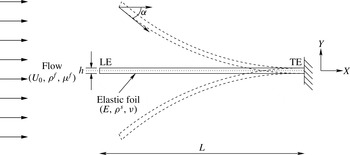
. As shown in figure 1, the trailing edge (TE) of the flexible foil is clamped and the leading edge (LE) is free to perform flapping motion. Here,
 $L$
and
 $h$
represent the length and thickness of the foil respectively,
 $U_{0}$
is the magnitude of the uniform axial flow exciting the flapping instability,
 ${\it\rho}^{f}$
and
 ${\it\rho}^{s}$
are the densities of the fluid and structure,
 ${\it\mu}^{f}$
denotes the fluid dynamic viscosity,
 ${\it\alpha}$
represents the leading edge angle of attack,
 $E$
is Young’s modulus and
 ${\it\nu}$
is the Poisson’s ratio of the foil.
Schematic of an inverted flexible foil of length
 $L$
and thickness
 $h$
in uniform axial flow
 $U_{0}$
with the leading edge (LE) free to oscillate and the trailing edge (TE) clamped.

The Navier–Stokes equations governing an incompressible flow in an arbitrary Lagrangian–Eulerian reference frame are
 $$\begin{eqnarray}\displaystyle & \displaystyle {\it\rho}^{f}\frac{\partial \boldsymbol{u}^{f}}{\partial t}+{\it\rho}^{f}\left(\boldsymbol{u}^{f}-\boldsymbol{w}\right)\boldsymbol{\cdot }\boldsymbol{{\rm\nabla}}\boldsymbol{u}^{f}=\boldsymbol{{\rm\nabla}}\boldsymbol{\cdot }{\bf\sigma}^{f}+\boldsymbol{f}^{f}\quad \text{in }{\it\Omega}^{f}(t), & \displaystyle\end{eqnarray}$$
 $$\begin{eqnarray}\displaystyle & \displaystyle \boldsymbol{{\rm\nabla}}\boldsymbol{\cdot }\boldsymbol{u}^{f}=0\quad \text{in }{\it\Omega}^{f}(t), & \displaystyle\end{eqnarray}$$
 $\boldsymbol{u}^{f}=\boldsymbol{u}^{f}(\boldsymbol{x},t)$
and
 $\boldsymbol{w}=\boldsymbol{w}(\boldsymbol{x},t)$
represent the fluid and mesh velocities defined for each spatial point
 $\boldsymbol{x}\in {\it\Omega}^{f}(t)$
respectively,
 $\boldsymbol{f}^{f}$
is the body force applied on the fluid and
 ${\bf\sigma}^{f}$
is the Cauchy stress tensor for a Newtonian fluid, written as
 $$\begin{eqnarray}{\bf\sigma}^{f}=-p\unicode[STIX]{x1D644}+\unicode[STIX]{x1D64F},\quad \unicode[STIX]{x1D64F}=2{\it\mu}^{f}{\bf\epsilon}^{f}(\boldsymbol{u}^{f}),\quad {\bf\epsilon}^{f}(\boldsymbol{u}^{f})={\textstyle \frac{1}{2}}[\boldsymbol{{\rm\nabla}}\boldsymbol{u}^{f}+(\boldsymbol{{\rm\nabla}}\boldsymbol{u}^{f})^{\text{T}}],\end{eqnarray}$$
where
 $p$
is the fluid pressure,
 $\unicode[STIX]{x1D644}$
denotes the second-order identity tensor and
 $\unicode[STIX]{x1D64F}$
represents the fluid viscous stress tensor. The deformation of the flexible foil is governed by the structural equation
 $$\begin{eqnarray}{\it\rho}^{s}\frac{\partial \boldsymbol{u}^{s}}{\partial t}=\boldsymbol{{\rm\nabla}}\boldsymbol{\cdot }{\bf\sigma}^{s}+\boldsymbol{f}^{s}\quad \text{in }{\it\Omega}^{s},\end{eqnarray}$$
where
 $\boldsymbol{u}^{s}=\boldsymbol{u}^{s}(\boldsymbol{z},t)$
is the structural velocity defined for each material point
 $\boldsymbol{z}\in {\it\Omega}^{s}$
,
 $\boldsymbol{f}^{s}$
represents the external forces applied on the solid and
 ${\bf\sigma}^{s}$
denotes the first Piola–Kirchhoff stress tensor. In this study, the structural stress tensor is modelled using the Saint Venant–Kirchhoff model (Antman Reference Antman1995). The coupled system required to satisfy the velocity and traction continuity conditions along the fluid–structure interface is as follows:
 $$\begin{eqnarray}\displaystyle & \displaystyle \int _{{\bf\varphi}^{s}({\it\gamma},t)}{\bf\sigma}^{f}({\bf\varphi}^{s}(\boldsymbol{z},t),t)\boldsymbol{\cdot }\boldsymbol{n}^{f}\,\text{d}{\it\Gamma}+\int _{{\it\gamma}}{\bf\sigma}^{s}(\boldsymbol{z},t)\boldsymbol{\cdot }\boldsymbol{n}^{s}\,\text{d}{\it\Gamma}=0\quad \forall {\it\gamma}\subset {\it\Gamma}_{0}, & \displaystyle\end{eqnarray}$$
 $$\begin{eqnarray}\displaystyle & \displaystyle \boldsymbol{u}^{f}({\bf\varphi}^{s}(\boldsymbol{z},t),t)=\boldsymbol{u}^{s}(\boldsymbol{z},t)\quad \forall \boldsymbol{z}\in {\it\Gamma}_{0}, & \displaystyle\end{eqnarray}$$
 $\boldsymbol{n}^{f}$
and
 $\boldsymbol{n}^{s}$
are respectively the outward normals to the deformed fluid and the undeformed solid interface boundaries,
 ${\it\Gamma}_{0}$
denotes the fluid–structure interface
 ${\it\Gamma}(t)$
at time
 $t=0$
and
 ${\bf\varphi}^{s}$
is the displacement function that maps each Lagrangian point
 $\boldsymbol{z}\in {\it\Omega}^{s}$
to its deformed position at time
 $t$
. Here,
 ${\it\gamma}$
is any part of interface
 ${\it\Gamma}_{0}$
and
 ${\bf\varphi}^{s}({\it\gamma},t)$
represents the corresponding fluid part over the interface
 ${\it\Gamma}(t)$
at time
 $t$
.
3. Coupled fluid–structure formulation
We employ a high-order variational method stable for very low mass ratios based on the CFEI formulation. In Liu et al. (Reference Liu, Jaiman and Gurugubelli2014), we have proved the numerical stability of the formulation for low structure-to-fluid mass ratio through energy estimates and demonstrated the ability of the scheme to simulate flapping dynamics. In this formulation, the solid positions and arbitrary Lagrangian–Eulerian mesh velocities are decoupled from the remaining variables (i.e. fluid velocity, pressure and structural velocity) and are handled explicitly. Consequently, the CFEI formulation only requires a linear system of equations to be solved for each time step. This step significantly decreases the size of the matrix that needs to be solved at each time step.
The weak form of the Navier–Stokes equations (2.1) and (2.2) can be written as
 $$\begin{eqnarray}\displaystyle & & \displaystyle \int _{{\it\Omega}^{f}(t)}{\it\rho}^{f}(\partial _{t}\boldsymbol{u}^{f}+(\boldsymbol{u}^{f}-\boldsymbol{w})\boldsymbol{\cdot }\boldsymbol{{\rm\nabla}}\boldsymbol{u}^{f})\boldsymbol{\cdot }{\bf\phi}^{f}\,\text{d}{\it\Omega}+\int _{{\it\Omega}^{f}(t)}{\bf\sigma}^{f}\boldsymbol{ : }\boldsymbol{{\rm\nabla}}{\bf\phi}^{f}\,\text{d}{\it\Omega}\nonumber\\ \displaystyle & & \displaystyle \quad =\int _{{\it\Omega}^{f}(t)}\boldsymbol{f}^{f}\boldsymbol{\cdot }{\bf\phi}^{f}\,\text{d}{\it\Omega}+\int _{{\it\Gamma}_{n}^{f}(t)}\boldsymbol{T}^{f}\boldsymbol{\cdot }{\bf\phi}^{f}\,\text{d}{\it\Gamma}+\int _{{\it\Gamma}(t)}({\bf\sigma}^{f}(\boldsymbol{x},t)\boldsymbol{\cdot }\boldsymbol{n}^{f})\boldsymbol{\cdot }{\bf\phi}^{f}(\boldsymbol{x})\,\text{d}{\it\Gamma},\end{eqnarray}$$
 $$\begin{eqnarray}\int _{{\it\Omega}^{f}(t)}q\boldsymbol{{\rm\nabla}}\boldsymbol{\cdot }\boldsymbol{u}^{f}\,\text{d}{\it\Omega}=0.\end{eqnarray}$$
Here,
 $\partial _{t}$
denotes the partial time derivative operator
 $\partial (\boldsymbol{\cdot })/\partial t$
,
 ${\bf\phi}^{f}\in H^{1}({\it\Omega}^{f}(t))$
and
 $q\in L^{2}({\it\Omega}^{f}(t))$
are the smooth test functions in the Sobolev space for the fluid velocity and pressure respectively,
 ${\it\Gamma}_{n}^{f}(t)$
represents the fluid Neumann boundary along which
 ${\bf\sigma}^{f}(\boldsymbol{x},t)\boldsymbol{\cdot }\boldsymbol{n}^{f}=\boldsymbol{T}^{f}$
. The weak form of the structural dynamics equation (2.4) can be written as
 $$\begin{eqnarray}\displaystyle & & \displaystyle \int _{{\it\Omega}^{s}}{\it\rho}^{s}\partial _{t}\boldsymbol{u}^{s}\boldsymbol{\cdot }{\bf\phi}^{s}\,\text{d}{\it\Omega}+\int _{{\it\Omega}^{s}}{\bf\sigma}^{s}\boldsymbol{ : }\boldsymbol{{\rm\nabla}}{\bf\phi}^{s}\,\text{d}{\it\Omega}\nonumber\\ \displaystyle & & \displaystyle \quad =\int _{{\it\Omega}^{s}}\boldsymbol{f}^{s}\boldsymbol{\cdot }{\bf\phi}^{s}\,\text{d}{\it\Omega}+\int _{{\it\Gamma}_{n}^{s}}\boldsymbol{T}^{s}\boldsymbol{\cdot }{\bf\phi}^{f}\,\text{d}{\it\Gamma}+\int _{{\it\Gamma}_{0}}\left({\bf\sigma}^{s}(\boldsymbol{z},t)\boldsymbol{\cdot }\boldsymbol{n}^{s}\right)\boldsymbol{\cdot }{\bf\phi}^{s}(\boldsymbol{z})\,\text{d}{\it\Gamma},\end{eqnarray}$$
where
 ${\bf\phi}^{s}\in H^{1}({\it\Omega}^{s})$
denotes a smooth test function for the structural velocity. Similarly to the fluid domain,
 ${\it\Gamma}_{n}^{s}$
represents the solid Neumann boundary and
 ${\bf\sigma}^{s}(\boldsymbol{z},t)\boldsymbol{\cdot }\boldsymbol{n}^{s}=\boldsymbol{T}^{s}$
. The weak form of the traction continuity condition along the fluid–structure interface (2.5) is given by
 $$\begin{eqnarray}\int _{{\it\Gamma}(t)}({\bf\sigma}^{f}(\boldsymbol{x},t)\boldsymbol{\cdot }\boldsymbol{n}^{f})\boldsymbol{\cdot }{\bf\phi}^{f}(\boldsymbol{x})\,\text{d}{\it\Gamma}+\int _{{\it\Gamma}_{0}}({\bf\sigma}^{s}(\boldsymbol{z},t)\boldsymbol{\cdot }\boldsymbol{n}^{s})\boldsymbol{\cdot }{\bf\phi}^{s}(\boldsymbol{z})\,\text{d}{\it\Gamma}=0.\end{eqnarray}$$
In the above equation, one may observe that
 $\boldsymbol{u}^{f}$
and
 $\boldsymbol{u}^{s}$
are defined on different domains
 ${\it\Omega}^{f}(t)$
and
 ${\it\Omega}^{s}$
respectively, and the condition
 $$\begin{eqnarray}{\bf\phi}^{f}({\bf\varphi}^{s}(\boldsymbol{z},t))={\bf\phi}^{s}(\boldsymbol{z})\quad \forall \boldsymbol{z}\in {\it\Gamma}_{0},\end{eqnarray}$$
can be realized by considering a conforming mesh along the interface
 ${\it\Gamma}_{0}$
with
 ${\bf\varphi}^{s}(\boldsymbol{z},t)$
being the position vector of the deformed solid. We next enforce the weak form of the traction continuity condition in (3.4) to combine (3.1)–(3.3) to construct the weak form of the coupled fluid–structure. For the weak form (Temam Reference Temam2001) of the coupled fluid–structure formulation, let us introduce the finite-dimensional trial solution function space
 $\mathscr{S}$
along with the corresponding test function space
 $\mathscr{V}$
. The weak form of the formulation can be written as follows: find
 $(\boldsymbol{u}^{f},p,\boldsymbol{u}^{s})\in \mathscr{S}$
such that
 $\forall ({\bf\phi}^{f},q,{\bf\phi}^{s})\in \mathscr{V}$
 $$\begin{eqnarray}\displaystyle & & \displaystyle \int _{{\it\Omega}^{f}(t)}{\it\rho}^{f}(\partial _{t}\boldsymbol{u}^{f}(\boldsymbol{x},t)+(\boldsymbol{u}^{f}-\boldsymbol{w})\boldsymbol{\cdot }\boldsymbol{{\rm\nabla}}\boldsymbol{u}^{f})\boldsymbol{\cdot }{\bf\phi}^{f}(\boldsymbol{x})\,\text{d}{\it\Omega}+\int _{{\it\Omega}^{f}(t)}{\bf\sigma}^{f}\boldsymbol{ : }\boldsymbol{{\rm\nabla}}{\bf\phi}^{f}\,\text{d}{\it\Omega}\nonumber\\ \displaystyle & & \displaystyle \qquad -\int _{{\it\Omega}^{f}(t)}q\boldsymbol{{\rm\nabla}}\boldsymbol{\cdot }\boldsymbol{u}^{f}\,\text{d}{\it\Omega}+\int _{{\it\Omega}^{s}}{\it\rho}^{s}\partial _{t}\boldsymbol{u}^{s}\boldsymbol{\cdot }{\bf\phi}^{s}\,\text{d}{\it\Omega}+\int _{{\it\Omega}^{s}}{\bf\sigma}^{s}\boldsymbol{ : }\boldsymbol{{\rm\nabla}}{\bf\phi}^{s}\,\text{d}{\it\Omega}\nonumber\\ \displaystyle & & \displaystyle \quad =\int _{{\it\Omega}^{f}(t)}\boldsymbol{f}^{f}\boldsymbol{\cdot }{\bf\phi}^{f}\,\text{d}{\it\Omega}+\int _{{\it\Gamma}_{n}^{f}(t)}\boldsymbol{T}_{n}^{f}\boldsymbol{\cdot }{\bf\phi}^{f}\,\text{d}{\it\Gamma}+\int _{{\it\Omega}^{s}}\boldsymbol{f}^{s}\boldsymbol{\cdot }{\bf\phi}^{s}\,\text{d}{\it\Omega}+\int _{{\it\Gamma}_{n}^{s}}\boldsymbol{T}^{s}\boldsymbol{\cdot }{\bf\phi}^{s}\,\text{d}{\it\Gamma},\end{eqnarray}$$
and the velocity continuity condition is enforced in the function space (Liu et al.
Reference Liu, Jaiman and Gurugubelli2014). As mentioned earlier, the main feature of the CFEI scheme is to explicitly determine the solid positions and the ALE-mesh displacements at the start of each time step. This feature enables us to decouple the ALE-mesh field from the remaining fluid–structure variables (
 $\boldsymbol{u}^{f}$
,
 $p$
and
 $\boldsymbol{u}^{s}$
). The solid position,
 ${\bf\varphi}^{s,n}$
, for the
 $n$
th time step can be determined using the second-order Adam–Bashforth method,
 $$\begin{eqnarray}{\bf\varphi}^{s,n}={\bf\varphi}^{s,n-1}+\frac{3{\rm\Delta}t}{2}\boldsymbol{u}^{s,n-1}-\frac{{\rm\Delta}t}{2}\boldsymbol{u}^{s,n-2}.\end{eqnarray}$$
The ALE-mesh nodes on the fluid domain
 ${\it\Omega}^{f}(t)$
can be updated using a steady pseudo-elastic material model (Stein, Tezduyar & Benney Reference Stein, Tezduyar and Benney2003) given by
 $$\begin{eqnarray}\boldsymbol{{\rm\nabla}}\boldsymbol{\cdot }{\bf\sigma}^{m}=\mathbf{0},\end{eqnarray}$$
where
 ${\bf\sigma}^{m}$
is the stress experienced by the ALE mesh due to the strain induced by the interface deformation. Assuming that the ALE mesh behaves as a linearly elastic material, the stress experienced can be written as
 $$\begin{eqnarray}{\bf\sigma}^{m}=(1+{\it\tau}_{m})[(\boldsymbol{{\rm\nabla}}\boldsymbol{{\it\eta}}^{f}+(\boldsymbol{{\rm\nabla}}\boldsymbol{{\it\eta}}^{f})^{\text{T}})+(\boldsymbol{{\rm\nabla}}\boldsymbol{\cdot }\boldsymbol{{\it\eta}}^{f})\unicode[STIX]{x1D644}],\end{eqnarray}$$
where
 $\boldsymbol{{\it\eta}}^{f}$
denotes the ALE-mesh nodal displacement satisfying the boundary conditions
 $$\begin{eqnarray}\displaystyle \boldsymbol{{\it\eta}}^{f}=\left\{\begin{array}{@{}ll@{}}{\bf\varphi}(\boldsymbol{z},t)-\boldsymbol{z}\quad & \forall \boldsymbol{z}\in {\it\Gamma}_{0},\\ 0\quad & \text{on}~{\it\Gamma}^{f}(t)\setminus {\it\Gamma}(t).\end{array}\right. & & \displaystyle\end{eqnarray}$$
Here,
 ${\it\Gamma}^{f}(t)$
is the fluid domain boundary and
 ${\it\Gamma}^{f}(t)\setminus {\it\Gamma}(t)$
denotes the non-interface fluid boundary;
 ${\it\tau}_{m}$
is a mesh stiffness variable chosen as a function of the element size to limit the distortion of the small elements located in the immediate vicinity of the fluid–structure interface. The mesh stiffness variable
 ${\it\tau}_{m}$
has been defined as
 ${\it\tau}_{m}=(\max _{i}|T_{i}|-\min _{i}|T_{i}|)/|T_{j}|$
, where
 $T_{j}$
represents the
 $j$
th element on the mesh
 $T$
.
The weak variational form in (3.6) is discretized in space using
 $\mathbb{P}_{n}/\mathbb{P}_{n-1}/\mathbb{P}_{n}$
isoparametric finite elements for the fluid velocity, pressure and solid velocity respectively. In this paper, we consider the stable
 $\mathbb{P}_{2}/\mathbb{P}_{1}/\mathbb{P}_{2}$
isoparametric finite-element meshes, which satisfy the inf–sup condition for well-posedness.
4. Numerical verification and convergence study
4.1. Numerical verification
To verify the coupled solver, we simulate a conventional flexible foil flapping in a uniform axial flow and compare our findings with the theoretical model and DNS results (Connell & Yue Reference Connell and Yue2007). The flapping dynamics of the conventional foil is strongly influenced by three critical non-dimensional parameters, namely
 $m^{\ast }$
,
 $\mathit{Re}$
and
 $K_{B}$
(Shelley et al.
Reference Shelley, Vandenberghe and Zhang2005; Connell & Yue Reference Connell and Yue2007), which are defined as
 $$\begin{eqnarray}\displaystyle m^{\ast }=\frac{{\it\rho}^{s}h}{{\it\rho}^{f}L},\quad K_{B}=\frac{B}{{\it\rho}^{f}U_{0}^{2}L^{3}},\quad \mathit{Re}=\frac{{\it\rho}^{f}U_{0}L}{{\it\mu}^{f}}. & & \displaystyle\end{eqnarray}$$
Here,
 $B$
represents the flexural rigidity defined as
 $B=Eh^{3}/12(1-{\it\nu}^{2})$
. The reduced velocity
 $U_{r}=\sqrt{m^{\ast }/K_{B}}$
can also be used to quantify the dynamic effects of flapping.
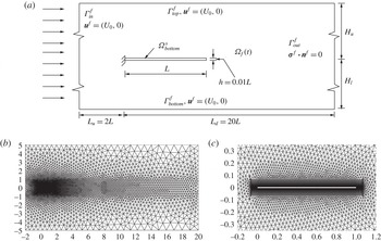
Conventional flexible foil system: (a) schematic and computational domain with details of boundary conditions; (b,c) unstructured high-order
 $\mathbb{P}^{2}/\mathbb{P}^{1}$
finite-element mesh corresponding to the flow domain with a single flexible foil in its undeformed configuration.

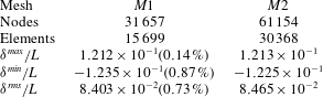
Mesh convergence study of conventional foil: comparison of non-dimensional tip-displacement statistics over
 $tU_{0}/L\in [15,20]$
for meshes
 $M1$
and
 $M2$
at
 $m^{\ast }=0.1,\mathit{Re}=1000$
and
 $K_{B}=0.0001$
. A constant time-step size
 ${\rm\Delta}t=0.001$
is employed.

We consider a two-dimensional computational domain of size
 $[22L\times 10L]$
, as shown in figure 2(a). In this computational domain, a flexible foil of length
 $L$
and thickness
 $h$
is placed along the
 $x$
-axis with its leading edge clamped and centred at
 $(0,0)$
. In figure 2(a),
 ${\it\Gamma}_{\mathit{in}}^{f}$
and
 ${\it\Gamma}_{\mathit{out}}^{f}$
represent the inlet and outlet boundaries respectively. A uniform velocity
 $U_{0}$
has been considered at
 ${\it\Gamma}_{\mathit{in}}^{f}$
and a traction-free boundary condition has been implemented along the outlet. Here,
 ${\it\Gamma}_{\mathit{top}}^{f}$
and
 ${\it\Gamma}_{\mathit{bottom}}^{f}$
denote the sides of the computational domain and the slip-wall condition has been implemented along these boundaries;
 $H_{u}$
and
 $H_{l}$
denote the spacings between the centreline of the foil and the domain boundaries
 ${\it\Gamma}_{\mathit{top}}^{f}$
and
 ${\it\Gamma}_{\mathit{bottom}}^{f}$
respectively. For this study, we consider a symmetric computational domain about the foil centreline i.e.
 $H_{u}=H_{l}=5L$
.
To select a suitable mesh for the simulation of the conventional foil, a mesh convergence study is performed for two different meshes
 $M1$
and
 $M2$
consisting of 15 699 and 30 368
 $\mathbb{P}_{2}/\mathbb{P}_{1}$
high-order triangular elements. The critical non-dimensional parameters considered for this study are
 $m^{\ast }=0.1,~K_{B}=0.0001$
and
 $\mathit{Re}=1000$
. A constant time-step size of
 ${\rm\Delta}t=0.001$
is employed with a characteristic time scale of
 $L/U_{0}$
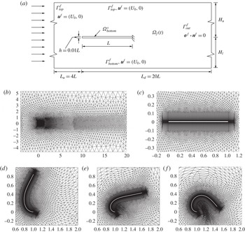
. Figures 2(b) and 2(c) show a typical high-order undeformed fluid mesh and a closeup view of the boundary layer mesh around the flexible foil respectively. Table 1 summarizes the trailing edge tip-displacement statistics for the meshes
 $M1$
and
 $M2$
. The values within the brackets represent the percentage difference in the numerical solutions with respect to the mesh
 $M2$
. The maximum difference between the numerical solutions calculated for the meshes
 $M1$
and
 $M2$
is less than 1 %. Therefore, the mesh
 $M1$
will be used in the numerical verification study.
First, we verify the ability of the coupled fluid–structure solver to predict the transition boundary from a stable mode to a flapping mode for a conventional flexible foil. An expression for the critical
 $K_{B}$
below which an infinitely wide conventional flexible foil loses its stability can be written as
 $$\begin{eqnarray}(K_{B})_{\mathit{cr}}=a-b\mathit{Re}^{-1/2},\end{eqnarray}$$
where
 $a=2m^{\ast }/(m^{\ast }k_{x}^{3}+2k_{x}^{2})$
and
 $b=C_{T}(2+m^{\ast }k_{x})/(m^{\ast }k_{x}^{3}+2k_{x}^{2})$
. Here,
 $C_{T}$
denotes the non-dimensional viscous tension coefficient which can be approximated to 1.328 with the aid of the laminar boundary layer theory (Connell & Yue Reference Connell and Yue2007). The above expression can be obtained by solving the quadratic dispersion relation
 $$\begin{eqnarray}\mathbb{D}=(m^{\ast }+2/k_{x}){\it\omega}^{2}-4{\it\omega}-C_{T}\mathit{Re}^{-1/2}k_{x}^{2}+2k_{x}-K_{B}k_{x}^{4}\end{eqnarray}$$
given by Connell & Yue (Reference Connell and Yue2007) for
 $\text{Im}({\it\omega})<0$
. For low
 $m^{\ast }$
, Connell & Yue (Reference Connell and Yue2007) and Shelley et al. (Reference Shelley, Vandenberghe and Zhang2005) have shown that a conventional flexible foil loses its stability when the fundamental mode
 $k_{x}=2{\rm\pi}$
becomes unstable. As part of this verification, we compare the critical
 $K_{B}$
observed from our DNS results with the analytical solutions of (4.2) for a range of
 $K_{B}$
and
 $\mathit{Re}$
at a fixed
 $m^{\ast }=0.1$
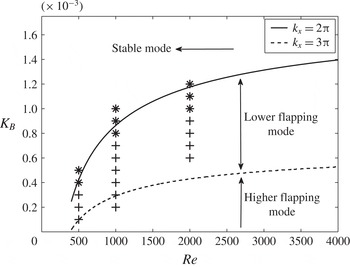
. Figure 3 summarizes our DNS results for
 $\mathit{Re}=500,\,1000$
and
 $2000$
in a stability phase diagram of a conventional foil. In this figure, the curve (——) represents the neutral curve between the stable and fundamental flapping modes, which is given by (4.2) for
 $k_{x}=2{\rm\pi}$
and
 $m^{\ast }=0.1$
. The curve (- - -) represents the transition between the fundamental mode
 $k_{x}=2{\rm\pi}$
and the higher mode
 $k_{x}=3{\rm\pi}$
given by (4.2) for
 $m^{\ast }=0.1$
. The stability phase diagram shows good agreement between our DNS and the analytical solution for
 $\mathit{Re}\leqslant 1000$
. To prove the existence of the fundamental mode
 $k_{x}=2{\rm\pi}$
and the transition from the fundamental mode
 $k_{x}=2{\rm\pi}$
to the higher mode
 $k_{x}=3{\rm\pi}$
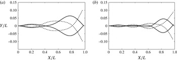
, we plot the full-body profiles of the flexible foil when the trailing edge is at its extrema and when it is crossing the mean position in figure 4 for
 $K_{B}=3.27\times 10^{-4}$
and
 $1.8\times 10^{-4}$
. From figure 4(a) at
 $K_{B}=3.27\times 10^{-4}$
, it can be inferred that the flapping modes range between
 $k_{x}=2{\rm\pi}$
and
 $5{\rm\pi}/2$
. Since
 $k_{x}=2{\rm\pi}$
represents the least stable mode of
 $k_{x}\in [2{\rm\pi},5{\rm\pi}/2]$
, the use of
 $k_{x}=2{\rm\pi}$
seems to be appropriate. For
 $K_{B}=1.8\times 10^{-4}$
, as shown in figure 4(b), the flexible foil exhibits flapping modes in the range
 $k_{x}\in [3{\rm\pi},7{\rm\pi}/2]$
, and the explanation given for
 $k_{x}=2{\rm\pi}$
can be extended to
 $k_{x}=3{\rm\pi}$
.
Stability phase diagram of a conventional foil at
 $m^{\ast }=0.1$
showing the critical neutral curve for
 $k_{x}=2{\rm\pi}$
(——) and
 $k_{x}=3{\rm\pi}$
(- - -) given by (4.2). Here,
 $+$
and
 $\ast$
represent the direct numerical simulation results corresponding to flapping and stable modes respectively.

Full-body profiles of conventional flexible foil performing flapping motion at
 $\mathit{Re}=1000$
,
 $m^{\ast }=0.1$
for
 $K_{B}=$
(a)
 $3.27\times 10^{-4}$
, (b)
 $1.8\times 10^{-4}$
.

Next, we assess the accuracy of the coupled solver in simulating the flapping dynamics of a conventional foil for
 $m^{\ast }=0.075$
,
 $\mathit{Re}=1000$
and
 $K_{B}=0.0001$
. In table 2, the key flapping properties for these cases are compared with the DNS results of Connell & Yue (Reference Connell and Yue2007) for identical non-dimensional simulation parameters. The values in the brackets indicate the percentage difference between the reference solution (Connell & Yue Reference Connell and Yue2007) and the current study. Despite different underlying structural formulations, fluid–structure coupling techniques and discretization methods, it can be observed that there is reasonable agreement among the flapping properties for both the mass ratios.
Numerical comparison against reference results of Connell & Yue (Reference Connell and Yue2007) at
 $\mathit{Re}=1000$
and
 $K_{B}=0.0001$
.

4.2. Mesh convergence of inverted foil
To examine the instability and post-critical nonlinear dynamics of an inverted flexible foil, we consider two computational domain configurations. The first computational domain will be used to study the initial development of instability in the inverted flexible foil. This computational domain is symmetrical about the foil centreline and is similar to the one presented earlier for the conventional foil, except that the trailing edge of the foil is clamped and the leading edge is free to oscillate. The converged finite-element mesh
 $M1$
defined for the conventional foil will be employed to simulate the evolution of flapping instability.
Inverted foil system: (a) representative schematic of the inverted foil computational set-up cantilevered at the trailing edge in a uniform axial flow; (b,c) typical representation of the high-order isoparametric finite-element mesh
 $M3$
, for the complete fluid domain (b) and closeup view of the central block and boundary layer mesh at the interface (c); (d–f) closeup view of the deformed mesh around the foil for
 $tU_{0}/L=7.3,~12$
and 17.

Figure 5(a) shows a typical schematic of the second computational domain, which will be used to simulate the post-critical flapping dynamics of the inverted foil. In contrast to the first computational domain, this domain is asymmetrical about the foil centreline i.e.
 $H_{u}\neq H_{l}$
. The size of the computational domain is
 $[24L\times 10L]$
, with
 $H_{u}=5.25L$
and
 $H_{l}=4.75L$
. The inverted flexible foil is neutrally stable in its undeformed state and it can bend on either side of its centreline. In order to have a numerically repeatable solution, we have considered a non-symmetrical computational domain. To study the influence of domain size for
 $K_{B}=0.2,~\mathit{Re}=1000$
and
 $m^{\ast }=0.1$
, two different domain widths,
 $10L$
and
 $40L$
, have been selected for assessment of the flapping response dynamics. The difference in the maximum tip displacement
 ${\it\delta}_{\mathit{max}}$
has been found to be less than 1 %. The maximum blockage ratio, which is defined as
 ${\it\delta}_{\mathit{max}}/(H_{u}+H_{l})$
, has been observed to be approximately 8.5 % and 2.125 % for the two domains respectively.
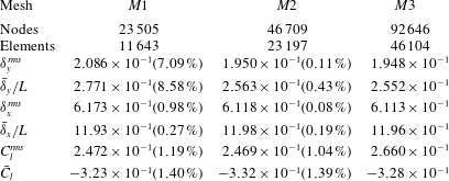
We next perform a detailed mesh convergence study for the asymmetrical computational domain using meshes
 $M1,~M2$
and
 $M3$
consisting of 11 643, 23 197 and 46 104
 $\mathbb{P}_{2}/\mathbb{P}_{1}$
triangular elements. A typical undeformed high-order finite-element fluid mesh
 $M3$
and the corresponding central block consisting of the boundary layer mesh can be seen in figure 5(b). Figure 5(c) shows a closeup view of the deformed mesh around the flexible foil for three time instants. For the purpose of mesh convergence study, we consider a flexible foil with
 $m^{\ast }=0.1$
and
 $K_{B}=10^{-4}$
interacting with fluid flow at
 $U_{0}=1$
corresponding to
 $\mathit{Re}=1000$
. A constant time-step size
 ${\rm\Delta}t=0.001$
has been employed. Table 3 summarizes the results of the mesh independence test for the inverted foil. The values within the brackets indicate the percentage difference in the numerical solutions with respect to the mesh
 $M3$
. The r.m.s. value of the cross-stream tip displacement is calculated using
 ${\it\delta}^{rms}/L=\sqrt{(1/n)\sum _{t=15\rightarrow 25}({\it\delta}^{\ast }-\bar{{\it\delta}}^{\ast })^{2}}$
, where
 ${\it\delta}^{\ast }$
is the non-dimensional tip displacement defined as
 ${\it\delta}/L$
and
 $\bar{{\it\delta}}^{\ast }$
denotes the non-dimensional mean tip displacement. A similar definition has been used to calculate
 $C_{l}^{rms}$
. Therefore, the mesh
 $M2$
will be employed to simulate the post-critical flapping dynamics of the inverted flexible foil.
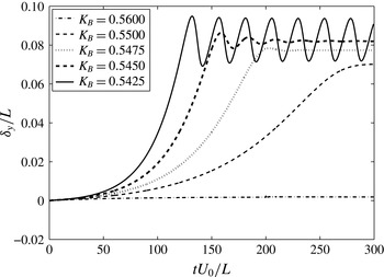
Time history of the leading edge cross-stream tip displacements for small changes in the non-dimensional bending rigidity
 $K_{B}$
at fixed
 $m^{\ast }=0.1$
and
 $\mathit{Re}=1000$
.

Inverted foil mesh convergence study: comparison of leading edge tip displacement and lift statics over
 $tU_{0}/L\in [20,30]$
for the meshes
 $M1,~M2$
and
 $M3$
at
 $m^{\ast }=0.1,~\mathit{Re}=1000$
and
 $K_{B}=0.01$
.

5. Flapping dynamics of inverted foil
5.1. Development of flapping instability
After establishing the validity of the numerical simulations, we present an underlying physical mechanism of the flapping instability for an inverted flexible foil. The symmetrical computational domain with
 $H_{u}=H_{l}=5L$
has been considered for this study. We first examine the evolution of the flapping instability as a function of
 $K_{B}$
for a fixed
 $m^{\ast }=0.1$
and
 $\mathit{Re}=1000$
by gradually decreasing
 $K_{B}$
from 0.8 to 0.2. Figure 6 shows the time history of the cross-stream leading edge displacements for
 $K_{B}=0.56,~0.55,~0.5475,~0.545$
and
 $0.5425$
. From this figure, we can identify three distinct stability regimes: (i) fixed-point stable, (ii) deformed steady state and (iii) unsteady flapping regime. In the first regime, for
 $K_{B}\geqslant 0.56$
, the flexible foil remains steady in its initial configuration with negligibly small leading edge cross-stream displacements. In the second regime, for
 $0.56<K_{B}<0.5425$
, the flexible foil deforms slowly to achieve a steady state. This steady state deformation increases with a decrease in
 $K_{B}$
. In the unsteady flapping regime, for
 $K_{B}\leqslant 0.5425$
, the flexible foil loses its stability, to perform regular sinusoidal oscillations with a constant frequency and amplitude.
5.1.1. Static divergence
The transition from the fixed-point stable to the deformed steady state regime can possibly be attributed to the static-divergence instability (Bisplinghoff, Ashley & Halfman Reference Bisplinghoff, Ashley and Halfman1957; Fung Reference Fung1969). We consider a simplified model of the static divergence by introducing a small normal impulsive force
 $P$
at the leading edge. As a result of this impulsive force, the flexible foil deforms with a leading edge cross-stream displacement
 ${\it\delta}_{y}$
and an angle of attack
 ${\it\alpha}$
. The inverted flexible foil will experience the static-divergence instability when the aerodynamic moment acting on it exceeds the elastic restoration moment (Fung Reference Fung1969). The aerodynamic moment can be evaluated by the lift force acting at the aerodynamic centre of the inverted flexible foil. The elastic restoration moment of the inverted flexible foil can be idealized as a spring connected at the leading edge. Therefore, the condition for the static divergence will be
 $$\begin{eqnarray}k{\it\delta}_{y}L<{\textstyle \frac{1}{2}}{\it\rho}^{f}U_{0}^{2}C_{l}({\it\alpha},\mathit{Re})Lx_{ac},\end{eqnarray}$$
where
 $k$
is the spring constant of an elastically mounted foil,
 $C_{l}$
is the lift coefficient expressed as function of
 $\mathit{Re}$
and
 ${\it\alpha}$
, and
 $x_{ac}$
denotes the distance between the aerodynamic centre and the trailing edge.
(a) Variation of
 $C_{l}$
as function of the leading edge angle of attack
 ${\it\alpha}$
at a fixed
 $\mathit{Re}=400$
and
 $m^{\ast }=0.1$
corresponding to the deformed steady state regime; (b) effect of
 $\mathit{Re}$
on
 $\partial C_{l}/\partial {\it\alpha}$
, where the curve (——) represents the empirical relation
 $a\mathit{Re}^{2}+b\mathit{Re}+c$
.

From the DNS results corresponding to the deformed steady state regime, we construct an empirical formulation for
 $C_{l}$
as a function of
 $\mathit{Re}$
and
 ${\it\alpha}$
. Figure 7(a) shows the relationship between
 $C_{l}$
and
 ${\it\alpha}$
obtained from the DNS simulations for a typical
 $\mathit{Re}=400$
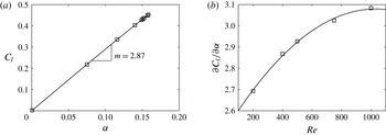
. From this figure, it can be noticed that
 $C_{l}$
is directly proportional to
 ${\it\alpha}$
and can be represented as
 $$\begin{eqnarray}C_{l}(\mathit{Re},{\it\alpha})=\frac{\partial C_{l}}{\partial {\it\alpha}}(\mathit{Re}){\it\alpha},\end{eqnarray}$$
where
 $(\partial C_{l}/\partial {\it\alpha})(\mathit{Re})$
denotes the slope of the curve in figure 7(a). Figure 7(b) shows the variation of
 $\partial C_{l}/\partial {\it\alpha}$
for a range of
 $\mathit{Re}$
, and the curve (——) represents the best-fit curve given by the equation
 $$\begin{eqnarray}\frac{\partial C_{l}}{\partial {\it\alpha}}(\mathit{Re})=a\mathit{Re}^{2}+b\mathit{Re}+c,\end{eqnarray}$$
where
 $a=-5.524\times 10^{-7}$
,
 $b=1.139\times 10^{-3}$
and
 $c=2.492$
. Therefore, (5.1) will be
 $$\begin{eqnarray}k{\it\delta}_{y}L<{\textstyle \frac{1}{2}}{\it\rho}^{f}U_{0}^{2}(a\mathit{Re}^{2}+b\mathit{Re}+c){\it\alpha}Lx_{ac}.\end{eqnarray}$$
On substituting
 $x_{ac}=3/4L$
,
 $k=3EI/L^{3},~{\it\delta}_{y}=PL^{3}/(3EI)$
and
 ${\it\alpha}=PL^{2}/(2EI)$
(Crandall, Dahl & Lardner Reference Crandall, Dahl and Lardner1995) in (5.4) and simplifying we obtain
 $$\begin{eqnarray}\frac{EI}{{\it\rho}^{f}U_{0}^{2}L^{3}}<\frac{3}{16}(a\mathit{Re}^{2}+b\mathit{Re}+c).\end{eqnarray}$$
The expression on the left-hand side represents
 $K_{B}$
from (4.1), and the critical
 $K_{B}$
for transition from the fixed-point stable to the deformed steady state regime will be
 $$\begin{eqnarray}(K_{B})_{\mathit{st}}={\textstyle \frac{3}{16}}(a\mathit{Re}^{2}+b\mathit{Re}+c).\end{eqnarray}$$
5.1.2. Stability regimes
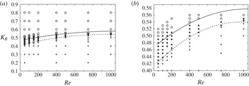
Figure 8 summarizes the stability regimes of an inverted flexible foil for a range of Reynolds numbers. In this figure, the curve (——) depicts
 $(K_{B})_{\mathit{st}}$
from (5.6) and the curve (- - -) represents the transition from the deformed steady state to the unsteady flapping regime given by the empirical relation
 $$\begin{eqnarray}(K_{B})_{f}=a^{\prime }\mathit{Re}^{2}+b^{\prime }\mathit{Re}+c,\end{eqnarray}$$
constructed based on the DNS results for a fixed
 $m^{\ast }=0.1$
, where
 $a^{\prime }=-1.39\times 10^{-7},~b^{\prime }=2.66\times 10^{-4}~\text{and}~c^{\prime }=0.41$
. From figure 8, we show that the static-divergence instability given by (5.6) is in good agreement with the DNS results and it characterizes the transition from the fixed-point stable to the deformed steady state regime.
Stability phase diagram: non-dimensional bending rigidity
 $K_{B}$
versus Reynolds number
 $\mathit{Re}$
for the inverted flexible foil at
 $m^{\ast }=0.1$
(a) and a closeup view of the phase diagram for
 $K_{B}\in [0.4,0.6]$
(b). The curves (——) and (- - -) represent the critical non-dimensional bending rigidity for static-divergence and flapping instability given by (5.6) and (5.7) respectively; ○,
 $\ast$
and
 $+$
denote the simulation results corresponding to the unstable flapping, steady deformed and fixed-point stable regimes.

As we decrease
 $K_{B}$
from 0.5450 to
 $0.5425$
for
 $\mathit{Re}=1000$
and
 $m^{\ast }=0.1$
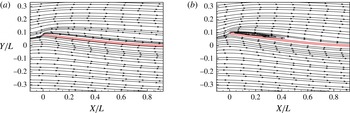
, the transition from the deformed steady state to the unsteady flapping regime is characterized by a leading edge separation which appears just before the foil attains its maximum deformation. This flow separation eventually reattaches around the half-location of the foil. Figure 9(b) shows the flow separation and reattachment along the foil for
 $K_{B}=0.5425$
at
 $tU_{0}/L=254$
, corresponding to the maximum transverse tip displacement. However, for
 $K_{B}=0.545$
the flow is observed to be fully attached without any flow reversal, which can be seen in figure 9(a). A flow separation at the leading edge results in a low-pressure region which increases the lift. Once the elastic restoring force becomes greater than the fluid force, the recoiling ability of the flexible foil results in suppression of the leading edge flow separation. At the instant when the flow is fully attached, the flexible foil once again experiences a static-divergence instability. Notably, there is still no detachment and convection of the leading edge vortex at
 $K_{B}=0.5425$
. However, on further decreasing the
 $K_{B}$
value a distinct leading edge vortex (LEV) develops and convects downstream. A discussion on the formation of the LEV is presented later in § 5.5.
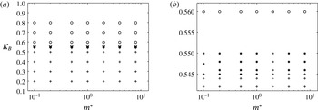
Furthermore, figure 10 summarizes the stability response regime map as a function of
 $m^{\ast }$
for a fixed
 $\mathit{Re}=1000$
. Interestingly, we observe that the effect of
 $m^{\ast }$
on both
 $(K_{B})_{\mathit{st}}$
and
 $(K_{B})_{f}$
is relatively small for
 $m^{\ast }\in [0.1,8]$
. It is observed that
 $(K_{B})_{\mathit{st}}\approx 0.56$
and
 $(K_{B})_{f}\approx 0.545$
for
 $\mathit{Re}=1000$
and
 $m^{\ast }\in [0.1,8]$
. We will further discuss the effects of mass ratio in § 5.3.
Instantaneous streamline contours at the leading edge corresponding to the maximum leading edge displacement for
 $K_{B}=$
(a)
 $0.545$
and (b)
 $0.5425$
;
 $m^{\ast }=0.1$
and
 $\mathit{Re}=1000$
.

Stability phase diagram as a function of the non-dimensional bending rigidity
 $K_{B}$
versus the mass ratio
 $m^{\ast }$
for an inverted flexible foil at
 $\mathit{Re}=1000$
(a) and a closeup view for
 $K_{B}\in [0.544,0.565]$
(b). Here, ○,
 $\ast$
and
 $+$
denote the simulation results corresponding to the unstable flapping, steady deformed and fixed-point stable regimes.

5.1.3. Conventional foil versus inverted foil
To understand why a conventional foil configuration does not experience a static divergence, we perform two sets of simulations on a fixed rigid flat plate at
 $\mathit{Re}=1000$
. In the first case, we rotate the rigid plate about the trailing edge to provide a small angle of attack,
 $5^{\circ }$
at the leading edge. For the second case, a small angle of attack,
 $-5^{\circ }$
, is provided at the leading edge by rotating about the leading edge. A symmetrical computational domain with
 $H_{u}=H_{l}=5L$
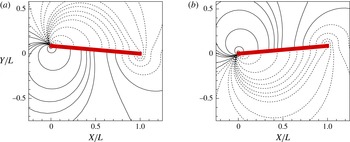
has been used for this study. Figure 11 shows the pressure distribution around the rigid plate for the two angle of attack cases. The first case with the positive angle of attack typically represents an inverted rigid plate experiencing a static divergence, whereas the second case represents a conventional rigid plate in a static divergence. For the first case, figure 11(a) shows that the lower surface is at a higher pressure than the upper surface. Hence, the aerodynamic lift acts in the direction of rotation and the rigid plate can undergo a static-divergence instability when the lift force crosses the critical restoring bending force (Fung Reference Fung1969). On the contrary, from figure 11(b) for the negative angle of attack, it can be observed that the nett aerodynamic lift acts in the direction opposite to the angle of rotation and has a stabilizing effect. Therefore, a cantilever beam clamped at the leading edge is less prone to a static-divergence instability.
Fluid pressure contours around a fixed rigid plate with (a) positive and (b) negative angle of attack for
 $\mathit{Re}=1000$
. The dashed lines represent negative pressure contours.

5.2. Effects of bending rigidity
Here, we present the flapping response results for an inverted flexible foil as a function of the non-dimensional bending rigidity
 $K_{B}\in [10^{-3},0.56]$
. We consider the asymmetric computational domain for this part of the study. The fluid and the structure parameters are
 $h=0.01L,~m^{\ast }=0.1$
and
 $\mathit{Re}=1000$
. From figure 3, it can be seen that the range of
 $K_{B}$
values selected for this study typically falls in the fixed-point regime for the conventional flexible foil.
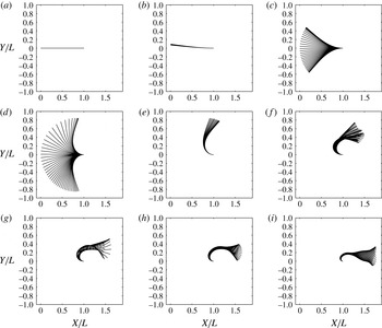
Full-body responses of an inverted flexible foil, plotted at
 ${\rm\Delta}tU_{0}/L=0.1$
at
 $\mathit{Re}=1000$
for
 $m^{\ast }=0.1$
and
 $K_{B}=$
(a) 0.56, (b) 0.5425, (c) 0.4, (d) 0.2, (e) 0.1, (f) 0.05, (g) 0.01, (h) 0.005 and (i) 0.001.

Three distinct unsteady flapping response regimes have been identified for
 $\mathit{Re}=1000$
and
 $m^{\ast }=0.1$
: (i) inverted limit-cycle oscillations for
 $0.545>K_{B}\geqslant 0.2$
, (ii) deformed flapping for
 $0.075<K_{B}\leqslant 0.1$
and (iii) flipped flapping for
 $K_{B}\leqslant 0.075$
. The above flapping response regimes have been classified based on the tip-displacement responses and the full-body profiles. Similar response regimes have been observed experimentally by Kim et al. (Reference Kim, Cossé, Huertas Cerdeira and Gharib2013) for mass ratios of
 $O(1)$
and
 $O(10^{-3})$
. In figure 12, we present the full-body profile results for
 $K_{B}\in [10^{-3},0.56]$
. Figure 12(a) shows the fixed-point stable foil profile in its undeformed state for
 $K_{B}=0.56$
. For
 $K_{B}\in [0.5425,0.2]$
, the flexible foil experiences the onset of flapping instability which develops into large-amplitude periodic oscillations, and this regime is defined as the inverted limit-cycle oscillations (LCO). Figure 12(b–d) shows typical full-body profiles for
 $K_{B}=0.5425,~0.4$
and
 $0.2$
over one oscillation cycle. During the initial stages of the inverted-LCO regime for
 $K_{B}\in [0.50,5425]$
the flexible foil does not perform flapping about the mean position, as shown in figure 12(b). However, for
 $K_{B}\in [0.5,0.2]$
the flexible foil performs flapping about its mean position. Moreover, from these figures, it can be observed that the inverted-LCO mode is predominantly the first mode and does not exhibit the typical necking phenomenon that is observed in a conventional foil (Huang Reference Huang1995; Liu et al.
Reference Liu, Jaiman and Gurugubelli2014). By decreasing the
 $K_{B}$
value, the flexible foil completely deforms to one direction and performs relatively small peak-to-peak amplitude oscillations as shown in figure 12(e). Due to the small peak-to-peak amplitudes, this regime has been described as a deformed mode by Kim et al. (Reference Kim, Cossé, Huertas Cerdeira and Gharib2013). Since the peak-to-peak amplitudes for this regime are of the same order as the amplitudes for a conventional foil flapping, we describe this regime as the deformed-flapping regime. By further decreasing the
 $K_{B}$
value, due to the low flexibility, part of the foil curves around the fixed edge to form a semicircular arc and the remaining part of the foil becomes parallel to the free stream velocity, as shown in figure 12(i). Figure 12(f–i) shows the full-body profiles for the inverted flexible foil for a range of
 $K_{B}<0.1$
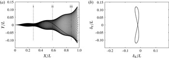
. The full-body profile shown in figure 12(i) closely resembles the full-body profile of the conventional foil shown in figure 13(a) for
 $K_{B}=3.27\times 10^{-4},~\mathit{Re}=1000$
and
 $m^{\ast }=0.1$
. Additionally, the necking phenomenon that is generally observed in the case of a conventional foil flapping has been observed in this regime. The maximum Reynolds numbers with respect to the semicircular arc diameter,
 $\mathit{Re}_{{\it\delta}}$
, is approximately 380 for
 $K_{B}=0.05$
, which signifies that our current two-dimensional simulations might not be able to capture the three-dimensional flow structures.
(a) Full-body profiles over one full cycle and (b) phase relation between the streamwise and cross-stream trailing edge tip displacements for a conventional foil with
 $K_{B}=3.27\times 10^{-4},~\mathit{Re}=1000$
and
 $m^{\ast }=0.1$
.

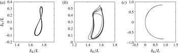
Phase plot of leading edge cross-stream and streamwise displacements for
 $K_{B}=$
(a) 0.001, (b) 0.01 and (c) 0.2 at
 $\mathit{Re}=1000$
and
 $m^{\ast }=0.1$
.

To further compare the flapping phenomenon in the flipped-flapping regime to the conventional foil, we plot the phase relation between the streamwise and the cross-stream tip displacements, as shown in figure 14. The phase plot for the flipped-flapping regime at
 $K_{B}=10^{-3}$
forms an eight-shaped figure (figure 14
a), which is similar to the phase relationship shown in figure 13(b) for the conventional foil with
 $K_{B}=3.27\times 10^{-4},~\mathit{Re}=1000$
and
 $m^{\ast }=0.1$
. The phase plot for the inverted LCO presents a unique parabolic profile, i.e. the leading edge follows the same path during the upward and downward strokes, which can be seen in figure 14(c) for
 $K_{B}=0.2$
. Moreover, no distinct phase plot has been observed for
 $K_{B}$
corresponding to the flipped-flapping regime, as shown in figure 14(a,b) for
 $K_{B}=0.01$
and
 $0.001$
respectively.
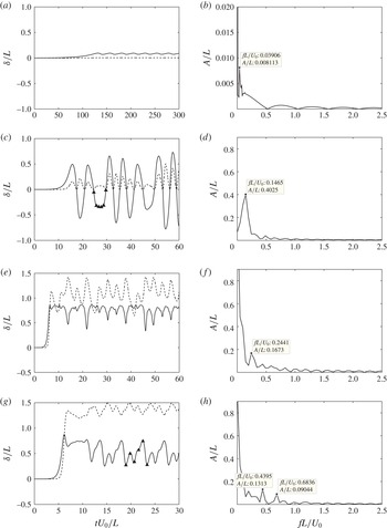
Time history of the cross-stream (——) and streamwise (- - -) leading edge tip displacement (a,c,e,g,i,k,m) and amplitude–frequency spectrum of the cross-stream leading edge tip displacement (b,d,f,h,j,l,n) for
 $K_{B}=$
(a,b) 0.5425, (c,d) 0.4, (e,f) 0.1, (g,h) 0.05, (i,j) 0.01, (k,l) 0.005 and (m,n) 0.001 at
 $\mathit{Re}=1000$
and
 $m^{\ast }=0.1$
. Here, ▴ represents the time instants for which vorticity contours will be presented in § 5.6.

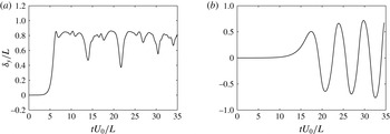
Figure 15 shows the time history of streamwise (- - -) and cross-stream (——) displacements along with the cross-stream amplitude–frequency spectrum. In this figure, ▴, represents the time instants for which vorticity contours will be presented in § 5.6. The leading edge tip displacements for the inverted-LCO regime exhibit a sudden rise when
 $K_{B}$
is decreased from 0.545 to 0.4, as shown in figure 15(a,b). Figure 15(c) shows the leading edge tip-displacement history for the deformed-flapping regime at
 $K_{B}=0.1$
. In this regime, the leading edge remains steady for a significant time period, which is followed by non-periodic oscillations with relatively small peak-to-peak amplitudes ranging between 0.2 and 0.4. Figure 15(d–g) shows the tip-displacement response history of the flipped-flapping regime. The flapping amplitudes for this regime are significantly smaller than those observed in the inverted-LCO regime and are approximately equal to those observed in the conventional foil. However, the flapping frequencies are smaller than those observed in the conventional foil flapping. The transition from the deformed-flapping to the flipped-flapping regime is predominantly characterized by two frequency oscillations, as shown in figure 15(d). The first low harmonic corresponds to the flapping frequency and the second frequency may be attributed to an additional higher-harmonic frequency of shear layer roll-up over the semicircular configuration. According to Strouhal’s law, it may be estimated as
 $f_{H}=St(U_{0}/D_{\mathit{foil}})$
, where
 $D_{\mathit{foil}}$
is the effective diameter of the semicircular body and
 $St$
is the Strouhal number. The higher harmonics 0.6838 and 1.025 appearing in figure 15(d,e) approximately coincide with the Strouhal frequencies corresponding to the vortex shedding of the semicircular body. In addition, we also observe a complex vortex–foil interaction and a reversed flow inside the deformed cavity-like region. A detailed investigation of these phenomena is beyond the scope of this study. The wake topology will be further illustrated in § 5.6 with the aid of the vorticity evolution in a flapping period. The high-harmonic frequency gets further damped as
 $K_{B}$
is lowered from 0.01 to 0.001, and the flapping response for
 $K_{B}=0.001$
exhibits a single distinct frequency (figure 15
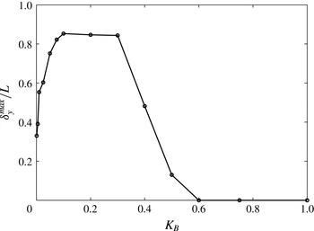
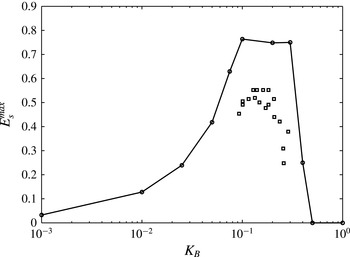
h). Figure 16 summarizes the effect of
 $K_{B}$
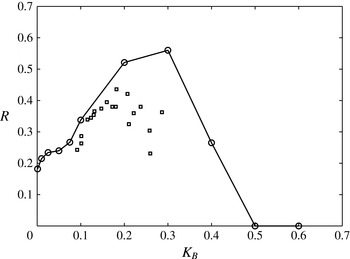
on the maximum leading edge cross-stream tip displacement. For large
 $K_{B}$
values, the flexible foil remains stable. A sharp rise in the maximum tip displacement can be observed for
 $K_{B}\in [0.3,0.5]$
. The maximum flapping amplitudes stabilize to an approximate value of
 $0.85$
, which is similar to the experimental observation made by Kim et al. (Reference Kim, Cossé, Huertas Cerdeira and Gharib2013).
5.3. Effects of mass ratio
To analyse the effects of mass ratio on the inverted flexible foil, we perform a series of numerical simulations for
 $m^{\ast }\in [0.1,10]$
. We first examine the effects of
 $m^{\ast }$
on the inverted-LCO regime for a fixed
 $K_{B}=0.4$
and
 $\mathit{Re}=1000$
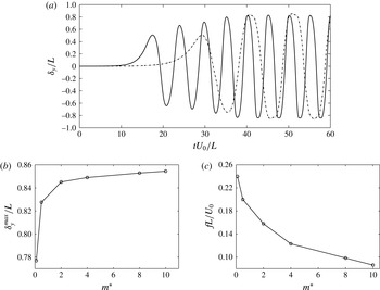
. Figure 17(a) shows the leading edge cross-stream tip-displacement history for
 $m^{\ast }=0.5$
and
 $8$
. From this figure, it can be seen that the flapping frequency is strongly influenced by the increase in
 $m^{\ast }$
, while the cross-stream flapping amplitudes are weakly affected. It may be noted that with increase in
 $m^{\ast }$
, the unsteady flapping instability takes a greater time to develop due to the inertial effects. Figure 17(b,c) summarizes the effect of
 $m^{\ast }$
on the flapping amplitudes and frequencies.
Maximum cross-stream displacement of the inverted foil leading edge centre over
 $tU_{0}/L\in [20,30]$
for
 $m^{\ast }=0.1,\mathit{Re}=1000$
and
 $K_{b}\in [0.001,1]$
.

Effect of the mass ratio
 $m^{\ast }$
on (a) the cross-stream leading edge tip displacements for
 $m^{\ast }=0.5$
(——) and
 $8$
(- - -), (b) the maximum cross-stream leading edge tip displacements and (c) the frequency, at a fixed
 $K_{B}=0.4$
and
 $\mathit{Re}=10\,000$
.

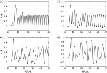
Time history of the cross-stream leading edge displacements for
 $m^{\ast }=$
(a) 0.1, (b) 0.5, (c) 1 and (d) 2, at a fixed
 $K_{B}=0.01$
and
 $\mathit{Re}=1000$
.

To understand the effects of
 $m^{\ast }$
on the flipped-flapping regime, we consider
 $K_{B}=0.01$
and
 $\mathit{Re}=1000$
for
 $m^{\ast }\in [0.1,2]$
. Figure 18 shows the leading edge cross-stream displacement histories for
 $m^{\ast }=0.1,~0.5,~1$
and 2. From figure 18(a,b), we observe regular periodic oscillations for
 $m^{\ast }=0.1$
and 0.5, which transform into non-periodic oscillations by increasing
 $m^{\ast }$
to 1. These non-periodic oscillations are characterized by variable amplitudes and frequencies. Figure 18(c,d) shows the non-periodic oscillations for
 $m^{\ast }=1$
and 2. A similar observation of transition from regular periodic to non-periodic oscillations with increase in
 $m^{\ast }$
was made by Connell & Yue (Reference Connell and Yue2007) for conventional foils.
Time history of the leading edge cross-stream displacements for
 $m^{\ast }=$
(a) 0.1 and (b) 0.5 at a fixed
 $K_{B}=0.1$
and
 $\mathit{Re}=1000$
.

The mass ratio
 $m^{\ast }$
can also affect the transition from the inverted-LCO to the deformed-flapping regime. Figure 19 shows the leading edge cross-stream displacements for
 $m^{\ast }=0.1$
and 0.5 for a fixed
 $K_{B}=0.1$
. With an increase in
 $m^{\ast }$
from 0.1 to 0.5, a delay in the transition from the inverted LCO to the deformed flapping can be seen in figure 19.
(a) A typical schematic of the inverted flexible foil in the curvilinear coordinate system with
 $s=0$
and
 $L$
at the trailing and leading edges; (b) a comparison between the simulated (- - -) foil profiles over one complete flapping cycle and the quasistatic equilibrium predicted (——) foil profile for
 $K_{B}=0.1,~\mathit{Re}=1000$
and
 $m^{\ast }=0.1$
.

5.4. Transition to deformed-flapping regime
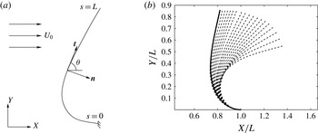
In the deformed-flapping regime, an inverted flexible foil deforms completely to one side and performs a flapping motion about the deformed position. To understand the transition from the inverted-LCO regime to the deformed-flapping regime, we perform a simple quasistatic equilibrium analysis. Figure 20(a) shows a typical schematic of an inverted flexible foil interacting with a uniform axial flow
 $U_{0}$
. We consider the curvilinear coordinates
 $(s,{\it\theta})$
, with
 $s=0$
and
 $L$
at the trailing and leading edges respectively;
 ${\it\theta}$
represents the local angle of incidence between the fluid flow and the unit tangent vector
 $\boldsymbol{t}$
. A flexible foil in quasistatic equilibrium should satisfy moment and force balance, which can be written in the dimensionless form as (Schouveiler, Eloy & Gal Reference Schouveiler, Eloy and Gal2005; Buchak et al.
Reference Buchak, Eloy and Reis2010)
 $$\begin{eqnarray}\frac{\text{d}{\it\theta}}{\text{d}s}=\frac{M}{K_{B}},\quad Q=\frac{\text{d}M}{\text{d}s},\quad \frac{\text{d}Q}{\text{d}s}=F+N,\end{eqnarray}$$
where the reference scales for length, time and mass are chosen as
 $L,L/U_{0}$
and
 ${\it\rho}^{f}L^{3}$
. Here,
 $M$
,
 $Q$
,
 $F$
and
 $N$
denote the internal moment, shear, inviscid and viscous fluid forces respectively. The non-dimensional fluid loading (Schouveiler et al.
Reference Schouveiler, Eloy and Gal2005) can be written as
 $$\begin{eqnarray}\displaystyle & \displaystyle N={\textstyle \frac{1}{2}}(C_{d}\sin ^{2}{\it\theta}+4\mathit{Re}^{-1/2}\sin ^{3/2}{\it\theta}), & \displaystyle\end{eqnarray}$$
 $$\begin{eqnarray}\displaystyle & \displaystyle F=-1.189\frac{\text{d}{\it\theta}}{\text{d}s}\cos ^{2}{\it\theta}, & \displaystyle\end{eqnarray}$$
 $C_{d}$
denotes the drag coefficient and
 $1.189{\it\rho}^{f}L$
represents the quasistatic fluid mass coefficient for a two-dimensional plate per unit width (Lighthill Reference Lighthill1960; Newman Reference Newman1977). The quasistatic equilibrium foil profile can be predicted by solving (5.8) along with the boundary conditions
 ${\it\theta}=0$
at
 $s=0$
,
 $M=0$
and
 $Q=0$
at
 $s=L$
. Figure 20(b) shows the predicted foil profile along with the DNS profiles for
 $K_{B}=0.1,~\mathit{Re}=1000$
,
 $m^{\ast }=0.1$
and
 $C_{d}=2.12$
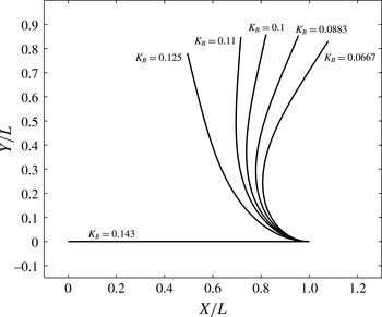
. From this figure, we can see that the flexible foil performs flapping about the quasistatic equilibrium state. Figure 21 presents superimposed quasistatic equilibrium foil profiles as a function of
 $K_{B}$
for a fixed
 $\mathit{Re}=1000$
and
 $C_{d}=2.12$
. This demonstrates the existence of a critical
 $K_{B}$
value of
 $0.125$
above which the flexible foil can no longer be supported by the fluid force. The quasistatic equilibrium between the restoring structural and fluid forces plays a role in the transition from the inverted-LCO to the deformed-flapping regime.
Superimposed views of the flexible foil profiles in the quasistatic equilibrium state for
 $K_{B}\in [0.066,0.125],~\mathit{Re}=1000$
and
 $C_{d}=2.12$
.

5.5. Formation of a leading edge vortex
The static divergence of an inverted flexible foil explains why the inverted foil is more prone to the flapping instability. However, this does not fully explain the cause of the large-amplitude oscillations observed in the case of the inverted limit-cycle flapping regime presented in § 5.2. The peak-to-peak amplitudes observed for this regime as a function of
 $K_{B}$
, for fixed
 $\mathit{Re}=1000$
and
 $m^{\ast }=0.1$
, are approximately six times greater than the peak-to-peak amplitudes observed for the conventional foil counterpart. Since vortex structures play a key role in determining the periodic loading on a flexible body, we analyse the wake topology for
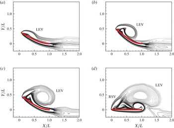
 $K_{B}=0.4$
, as shown in figure 22. A leading edge vortex (LEV) slowly develops behind the flexible foil during the upstroke. This leading edge vortex remains attached throughout the stroke and grows continuously until the leading edge reaches the maximum displacement prior to the stroke reversal. At the stroke reversal, the leading edge vortex pairs up with a counter-rotating vortex from the lower surface of the foil at the trailing edge and is shed into the wake. Meanwhile, a rotational starting vortex (RSV) is being formed at the leading edge, as shown in figure 22(c,d). The fact that the leading edge vortex produces a large low-pressure region behind the flexible foil results in large-amplitude oscillations. Similar leading edge vortices have been observed in the cases of insect flight (Wang Reference Wang2000) and delta wings (Ol & Gharib Reference Ol and Gharib2003). These leading edge vortices are generally attributed to the effective aerodynamic behaviour observed in the case of insect flight.
Evolution of the leading edge vortex (LEV) for the inverted-LCO regime at
 $K_{B}=0.4$
,
 $\mathit{Re}=1000$
and
 $m^{\ast }=0.1$
, with (a)
 $tU_{0}/L=10$
, (b)
 $tU_{0}/L=12.5$
, (c)
 $tU_{0}/L=15$
and (d)
 $tU_{0}/L=17.5$
.

5.6. Vortex organization
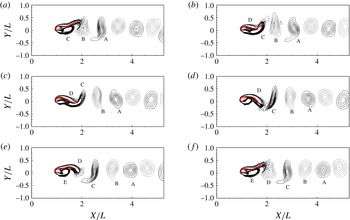
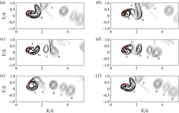
Vortex organization and formation are key to the understanding of many phenomena in fluid–structure interactions. Earlier studies have shown that a conventional flexible foil generates a regular von Kármán vortex street with two counter-rotating vortices. However, the flapping inverted foil exhibits a wide range of vortex patterns depending on the non-dimensional bending rigidity
 $K_{B}$
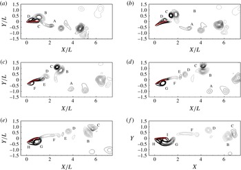
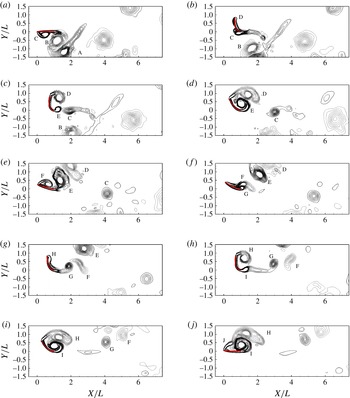
. Earlier, Kim et al. (Reference Kim, Cossé, Huertas Cerdeira and Gharib2013) observed that a pair of leading edge vortices are shed per one oscillation. In our numerical study, the number of leading edge vortex pairs can be greater than one during the flapping oscillation, as illustrated in figures 23 and 24.
Time history of a
 $2P+S$
vortex wake over a half-cycle for
 $K_{B}=0.4,~\mathit{Re}=1000$
and
 $m^{\ast }=0.1$
, with (a)
 $tU_{0}/L=24.7~(0)$
, (b)
 $tU_{0}/L=25.7~(T_{0}/10)$
, (c)
 $tU_{0}/L=26.7~(2T_{0}/10)$
, (d)
 $tU_{0}/L=27.7~(3T_{0}/10)$
, (e)
 $tU_{0}/L=28.7~(4T_{0}/10)$
and (f)
 $tU_{0}/L=29.7~(5T_{0}/10)$
. The non-dimensional time period
 $T_{0}=10$
for full oscillation.

Time history of a
 $3P+S$
vortex wake over a half-cycle for
 $K_{B}=0.2,~\mathit{Re}=1000$
and
 $m^{\ast }=0.1$
, with (a)
 $tU_{0}/L=18.3~(0)$
, (b)
 $tU_{0}/L=19.4~(T_{0}/18)$
, (c)
 $tU_{0}/L=20.5~(2T_{0}/18)$
, (d)
 $tU_{0}/L=21.6~(3T_{0}/18)$
, (e)
 $tU_{0}/L=22.7~(4T_{0}/18)$
, (f)
 $tU_{0}/L=23.8~(5T_{0}/18)$
, (g)
 $tU_{0}/L=24.9~(6T_{0}/18)$
, (h)
 $tU_{0}/L=26.0~(7T_{0}/18)$
, (i)
 $tU_{0}/L=27.1~(8T_{0}/18)$
and (j)
 $tU_{0}/L=28.2~(9T_{0}/18)$
. The non-dimensional time period,
 $T_{0}$
, for one full oscillation is 18.6.

For the fixed-point stable regime i.e. for
 $K_{B}\geqslant 0.545$
, the flow field typically represents the boundary layer flow over a flat plate. As the flow travels, a symmetric boundary layer flow can be observed on either side of the inverted foil, off the fixed trailing edge, to form a narrow and steady wake. This wake is very similar to the one observed for the case of the fixed-point regime of conventional flexible foil. By decreasing
 $K_{B}<0.545$
, the inverted flexible foil experiences large-amplitude oscillations with very low frequency. Figure 23 displays a sequence of plots showing the vorticity contours in the fluid for the case of
 $K_{B}=0.4$
over one downstroke cycle corresponding to time
 $tU_{0}/L\in [24.7,29.7]$
. In this figure, the solid and dashed lines represent the positively and negatively signed vortices. Figure 23(a) displays the instantaneous vorticity contour at
 $tU_{0}/L=24.7$
, as the foil is about to cross the line
 $Y/L=0$
. In this figure, the leading edge vortex (B) that is shed during the previous upstroke can be seen forming a vortex pair with the oppositely signed vortex (C) shed from the lower surface at the trailing edge. The rotation starting vortex (D) formed during the upstroke reversal is still attached to the foil as it crosses the centreline. In figure 23(b), the vortex pair (B)
 $+$
(C) is shed into the wake; meanwhile, the rotation starting vortex (D) travels downstream along the flexible foil. The vortex pairs (B)
 $+$
(C) rotate about each other and convect further downstream in the wake. As the flexible foil bends downwards, the leading edge vortex (G) can be seen developing in figure 23(c). In the meantime, the rotation starting vortex (D) is shed into the wake from the trailing edge and draws an oppositely signed vortex (E) from the lower surface of the flexible foil to form a vortex pair (D)
 $+$
(E). In figure 23(d), the flexible foil is at maximum displacement and the leading edge vortex (G) continues to grow behind the flexible foil on the lower surface and is just about to be shed into the wake. The boundary layer on the upper surface of the flexible foil consists of a significant amount of vorticity, and this vorticity is shed into the wake as the elongated vortex (F), as shown in figure 23(d). As the flexible foil rebounds from the maximum displacement, the leading edge vortex (G) is shed into the wake, as shown in figure 23(e). The approach of vortex (G) cuts the supply of vorticity to the vortex (F) from the boundary layer. Meanwhile, a new rotation starting vortex (H) can be seen developing behind the leading edge. The leading edge vortex (F) draws a negatively signed vortex (I) from the upper surface of the flexible foil at the trailing edge to form a vortex pair, similar to the vortex pair between the leading edge vortex (B) and (C), in figure 23(f). Figure 23(f) at
 $tU_{0}/L=29.7$
corresponds to the flexible foil crossing the line
 $Y/L=0$
in the opposite direction, which completes the half-flapping cycle. In addition, we can also observe that the positions of vortices (F), (I) and (H) around the flexible foil in figure 23(f) are similar to the positions of the vortices (B), (C) and (D) in figure 23(a) except that all of the vortices are reversed. In summary, we therefore see that two vortex pairs (B)
 $+$
(C) and (D)
 $+$
(E) and a single vortex (F) are shed into the wake, i.e. a total of five vortices are shed in a half-cycle.
Time history of the regular von Kármán vortex street for
 $K_{B}=0.001$
,
 $\mathit{Re}=1000$
and
 $m^{\ast }=0.1$
over one oscillation of the flexible foil, with (a)
 $tU_{0}/L=19.72~(0)$
, (b)
 $tU_{0}/L=20.04~(T_{0}/5)$
, (c)
 $tU_{0}/L=20.36~(2T_{0}/5)$
, (d)
 $tU_{0}/L=20.68~(3T_{0}/5)$
, (e)
 $tU_{0}/L=21.00~(4T_{0}/5)$
and (f)
 $tU_{0}/L=21.32~(T_{0})$
. The time period of the oscillation,
 $T_{0}$
, is 1.6.

The formation of
 $6P+2S$
wake structures observed for
 $K_{B}=0.2$
is shown in figure 24 over a half flapping cycle
 $tU_{0}/L\in [18.3,28.2]$
. In this figure, a leading edge vortex (A) forming a vortex pair with an oppositely signed vortex (B) shed from the top surface of the flexible foil and a rotation starting vortex (C) at the leading edge are indicated. In figure 24(b), the vortex pair (A)
 $+$
(B) is shed into the wake and the rotation starting vortex (C) travels downstream along the flexible foil. Meanwhile, a new leading edge vortex (D) can be seen developing in the background. In summary, we observe that vortex pairs (A)
 $+$
(B), (D)
 $+$
(E) and (F)
 $+$
(G) and a single vortex (C) are shed into the wake, i.e. seven vortices being shed in a half-cycle. In contrast to the experimental observations in Kim et al. (Reference Kim, Cossé, Huertas Cerdeira and Gharib2013), in this case we observe that a pair of leading edge vortices (D) and (H) are shed per half-cycle.
As explained earlier, in the case of the flipped-flapping regime the leading edge of the flexible foil curves around the trailing edge and performs a flapping motion behind the fixed trailing edge. In order to avoid any confusion, we refer to the trailing and leading edges as the fixed and flipped edges respectively. With regard to the wake patterns, the flipped-flapping regime is very similar to the limit-cycle regime of a conventional flexible foil. Figure 25 shows the time history of the steady von Kármán wake of the inverted flexible foil for the flipped-flapping regime with a single distinct frequency at
 $K_{B}=10^{-3}$
. This figure shows the instantaneous vorticity at six different points over one periodic oscillation. Figure 25(a) represents the instantaneous vorticity at
 $tU_{0}/L=19.72$
, corresponding to the condition when the leading edge is at its highest position; three vortices (A)–(C) close to the flipped leading edge and in the immediate downstream are shown. In figure 25(b), the positively signed vortex (A) and negatively signed vortex (B) convect further downstream. Meanwhile, the counter-rotating vortex (C) shed from the lower rounded surface gets reattached to the bottom surface of the flipped flexible foil. Two counter-rotating vortices are totally shed over one cycle.
Time history of a periodic wake containing four vortices over two complete oscillations for
 $K_{B}=0.05$
,
 $\mathit{Re}=1000$
and
 $m^{\ast }=0.1$
, with (a)
 $tU_{0}/L=18.98~(0)$
, (b)
 $tU_{0}/L=19.86~(T_{0}/5)$
, (c)
 $tU_{0}/L=20.74~(2T_{0}/5)$
, (d)
 $tU_{0}/L=21.62~(3T_{0}/5)$
, (e)
 $tU_{0}/L=22.50~(4T_{0}/5)$
and (f)
 $tU_{0}/L=23.38~(T_{0})$
. The non-dimensional time period for two complete oscillations,
 $T_{0}$
, is 3.4.

Figure 26 illustrates the time development of the wake topology consisting of a
 $2S+2S$
vortex pattern for the case of the flipped-flapping regime with two distinct frequencies at
 $K_{B}=0.05$
. In contrast to the flipped-flapping regime with a single frequency, the wake topology does not represent the von Kármán vortex street. However, a periodic vortex shedding repeats after two complete cycles. The vortex wake in figure 26(f) corresponding to
 $tU_{0}/L=23.38$
is very similar to the wake at
 $tU_{0}/L=18.98$
, and four vortices (B)–(E) are shed over two cycles. In the flipped-flapping regime, we observe complicated flow features, namely a rolled-up shear layer over the semicircular configuration, vortex–foil interaction and a reversed flow inside the deformed cavity-like region, which are not shown here in detail.
5.7. Net energy transfer
In order to analyse the ability of an inverted flexible foil to extract energy from the surrounding fluid flow, we provide a comparison between the energy harvesting estimates for the conventional and inverted flexible foil configurations for low
 $m^{\ast }=0.1$
.
Comparison between the time evolution of (a) the bending strain energy and (b) the work done by the fluid on the flexible foil for
 $K_{B}=3.27\times 10^{-4},~\mathit{Re}=1000$
and
 $m^{\ast }=0.1$
. (c–f) The full-body profiles of the conventional foil at (i)–(iv) in (a) respectively.

Dependence of the non-dimensional elastic strain energy on the bending rigidity
 $K_{B}$
in a conventional flexible foil. Here, (——) and (- - -) denote the maximum and r.m.s. energy at
 $\mathit{Re}=1000$
and
 $m^{\ast }=0.1$
.

5.7.1. Conventional flexible foil
Figure 27 shows the evolution of the non-dimensional bending strain energy
 $(E_{s})$
and the net work done
 $(W_{s})$
on a conventional foil for
 $K_{B}=3.27\times 10^{-4},~\mathit{Re}=1000$
and
 $m^{\ast }=0.1$
. Here,
 $E_{s}$
and
 $W_{s}$
are defined as
 $$\begin{eqnarray}E_{s}=\frac{\displaystyle \frac{1}{2}\int _{0}^{l}EI{\it\kappa}^{2}\,\text{d}l}{{\it\rho}^{f}U_{0}^{2}L^{2}}\quad \text{and}\quad W_{s}=\frac{\displaystyle \int _{0}^{t}\left(\int _{{\it\Gamma}}({\bf\sigma}^{f}\boldsymbol{\cdot }\boldsymbol{n})\boldsymbol{\cdot }\boldsymbol{u}^{f}\text{d}{\it\Gamma}\right)\text{d}t}{{\it\rho}^{f}U_{0}^{2}L^{2}},\end{eqnarray}$$
where
 $$\begin{eqnarray}{\it\kappa}=\frac{|\partial ^{2}f(x)/\partial x^{2}|}{[1+(\partial f(x)/\partial x)^{2}]^{3/2}}\end{eqnarray}$$
is the curvature of the deformed flexible foil and
 $f(x)$
is a piecewise polynomial function of sixth order that has been constructed to define the deformed foil profile at each time instant. The strain energy
 $E_{s}$
of the flexible foil oscillates about a non-zero mean with a maximum value of
 $O(10^{-4})$
. The frequency of
 $E_{s}$
oscillations is twice the flapping frequency of the foil. The full-body flapping profiles of the foil shown in figure 27(c–f) correspond to the points (i)–(iv) indicated in figure 27(a). The strain energy
 $E_{s}$
of the flexible foil attains a local minimum for the maximum deformation of the trailing edge. In contrast, the flexible foil reaches the maximum
 $E_{s}$
as the trailing edge is about to cross the centreline. The strain energy
 $E_{s}$
increases from a local minimum to a local maximum due to the work done by the fluid force on the flexible foil. The flexible foil eventually loses this attained strain energy
 $E_{s}$
by performing work on the surrounding fluid. Interestingly, for the conventional foil flapping, we observe that the work done by the fluid in developing the structural strain energy is greater than the work done by the structure on the fluid. Therefore, the work done by the fluid per oscillation is greater than zero i.e.
 ${\rm\Delta}W_{s}>0$
, and the nett work done by the fluid continuously increases with time at a constant rate, as shown in figure 27(b). This observation reveals that a conventional foil configuration behaves like a non-conservative system. The reason for
 ${\rm\Delta}W_{s}>0$
per oscillation cycle can be attributed to the non-conservative (dissipative) nature of the fluid force and the path followed by the conventional flexible foil. From figures 13 and 27(c–f), it can be realized that the conventional flexible foil does not follow an identical path during its upstroke and downstroke. Since the work done by a non-conservative force is path-dependent, the work done by the fluid is different from the work performed by the structure.
Comparison between (——) the bending strain energy (
 $E_{S}$
) and (- - -) the work done by the fluid (
 $W_{s}$
) over
 $tU_{0}/L\in [0,40]$
at
 $K_{B}=0.4$
and
 $\mathit{Re}=1000$
for
 $m^{\ast }=$
(a) 0.1 and (b) 8.

Figure 28 summarizes the maximum and r.m.s. non-dimensional strain energies as a function of
 $K_{B}\in [10^{-5},10^{-3}]$
for
 $\mathit{Re}=1000$
and
 $m^{\ast }=0.1$
. For sufficiently large
 $K_{B}$
corresponding to the steady stable mode, the maximum and r.m.s. bending strain energies are close to zero. However, for
 $K_{B}$
corresponding to the unsteady flapping regime i.e.
 $K_{B}<7.0\times 10^{-4}$
, the maximum and r.m.s. strain energy values are of
 $O(10^{-4})$
. The sudden drop in the strain energy for
 $K_{B}<3.27\times 10^{-4}$
can be attributed to the transition from the fundamental mode
 $k_{x}=2{\rm\pi}$
to the higher
 $3{\rm\pi}$
flapping mode. By comparing local maximum strain energies for
 $K_{B}\in [7.5\times 10^{-5},3\times 10^{-4}]$
and
 $[3\times 10^{-4},7\times 10^{-4}]$
, we can conclude that lower flapping modes can extract greater bending strain energy compared with the higher bending mode.
In order to determine the effectiveness of the flapping phenomenon in extracting energy, we define the ratio of the maximum strain energy to the total available fluid kinetic energy as
 $$\begin{eqnarray}R=\frac{({\rm\Delta}E_{s})^{\mathit{max}}}{{\textstyle \frac{1}{2}}{\it\rho}^{f}U_{0}^{2}{\it\delta}_{y}^{\mathit{max}}T},\end{eqnarray}$$
where
 $({\rm\Delta}E_{s})^{\mathit{max}}$
is the maximum change in the strain energy per oscillation,
 ${\it\delta}_{y}^{\mathit{max}}$
represents the maximum tip displacement and
 $T$
is the time taken to complete one half-cycle. As a typical case we consider
 $K_{B}=3.27\times 10^{-4}$
, which exhibits maximum non-dimensional bending strain energy, to examine the effectiveness of conventional flexible foils at low
 $m^{\ast }$
. On substituting
 ${\it\delta}_{y}^{\mathit{max}}=0.12$
,
 ${\rm\Delta}E_{s}^{\mathit{max}}=2.3\times 10^{-4}$
,
 ${\it\rho}^{f}=1000$
and
 $T=0.4$
observed from the DNS results for
 $K_{B}=3.27\times 10^{-4}$
, we obtain
 $R=O(10^{-7})$
, which is negligibly small. Therefore, we show that even though conventional foil can be used to harvest the energy from surrounding fluid flows, the effectiveness of a conventional flexible foil for low
 $m^{\ast }<1$
in extracting energy from the surrounding fluid flow is very low. A similar observation has been made by Michelin & Doare (Reference Michelin and Doare2013) for
 $m^{\ast }<1$
.
5.7.2. Inverted flexible foil
Figure 29(a,b) shows the evolution of the non-dimensional bending strain energy (
 $E_{s}$
) and the work done by the fluid force
 $(W_{s})$
on the inverted flexible foil for
 $tU_{0}/L\in [0,40]$
for
 $K_{B}=0.4,~\mathit{Re}=1000$
and
 $m^{\ast }=0.1$
and
 $8$
. Interestingly, we observe that
 $W_{s}$
closely follows
 $E_{s}$
in both of the cases. However, the contribution of the structural kinetic energy to the bending strain energy increases with
 $m^{\ast }$
. The magnitude of the strain energy developed in the inverted foil is typically
 $O(10^{3})$
times the value observed for the conventional foil. In contrast to the
 $E_{s}$
of the conventional foil, the
 $E_{s}$
of the inverted foil attains a local maximum for the maximum deformation of the leading edge and a local minimum as the leading edge crosses the centreline. Since the inverted-LCO regime of the inverted foil flapping follows an identical path for both the upstroke and the downstroke (figure 14
c), the work performed by the fluid will be the same as the work done by the structure. Therefore, we can observe from figure 29(a,b) that
 ${\rm\Delta}W_{s}\approx 0$
per cycle for
 $tU_{0}/L\geqslant 30$
when
 $m^{\ast }=0.1$
and for
 $tU_{0}/L\geqslant 48.6$
when
 $m^{\ast }=8$
. The inverted-LCO flapping regime represents a conservative system, i.e.
 ${\rm\Delta}W_{s}\approx 0$
per cycle, and is more effective in extracting the energy from the surrounding fluid flow in comparison to the conventional foil.
Maximum strain energy for the inverted flexible foil as a function of the non-dimensional bending rigidity for
 $tU_{0}/L\in [0,30]$
. Here, ▫ denotes the experimental data reported in Kim et al. (Reference Kim, Cossé, Huertas Cerdeira and Gharib2013).

Figure 30 summarizes the maximum strain energy developed in a flexible foil as a function of
 $K_{B}\in [10^{-3},1]$
for
 $\mathit{Re}=1000$
and
 $m^{\ast }=0.1$
. The experimental data (Kim et al.
Reference Kim, Cossé, Huertas Cerdeira and Gharib2013) corresponding to a higher mass ratio of
 $O(1)$
and Reynolds numbers of
 $O(10^{4})$
have also been shown for a qualitative comparison. It can be seen that both the experimental data and the current numerical simulation show a constant maximum strain energy for the inverted-LCO regime. However, the qualitative comparison shows that the current two-dimensional numerical simulations overestimate the maximum strain energy values. We attribute this difference to three-dimensional effects which have been neglected in the current numerical study. The aspect ratios of the flexible foils used in Kim et al. (Reference Kim, Cossé, Huertas Cerdeira and Gharib2013) were in the range of 1–1.3. In addition, we attribute the discrepancy in the maximum strain energy to the large difference in the mass ratio and the Reynolds numbers of the experimental study and the current numerical investigation. Another observation from figure 30 is that the maximum strain energy developed in the flipped-flapping regime is relatively smaller when compared with the inverted-LCO regime. However, the maximum strain energy developed in the flipped-flapping regime is still approximately
 $O(10^{3})$
times the maximum value developed in the conventional foil.
Figure 31 shows the ratio
 $R$
of the maximum bending strain energy to the total kinetic energy of the incoming fluid flow, as given in (5.12). It should be noted that (5.12) considers the maximum change in the
 $E_{s}$
per oscillation, i.e.
 $({\rm\Delta}E_{s})^{\mathit{max}}$
, instead of the total stored
 $E_{s}$
. Use of the total
 $E_{s}$
can include a large non-oscillatory part; however, that would not be useful for energy recovery. The effects of this consideration can be explained for the case of
 $K_{B}=0.1$
, corresponding to the deformed-flapping regime, where there is a large stored strain energy yet the total energy available for energy harvesting is much less than that of
 $K_{B}=0.2$
and 0.3. A comparison with the experimental data of Kim et al. (Reference Kim, Cossé, Huertas Cerdeira and Gharib2013) has also been presented in the figure. The energy efficiency ratio
 $R$
shows good agreement with the experimental data for
 $K_{B}\in [0.1,0.2]$
. We also observe a significant difference in the values for
 $K_{B}\in [0.2,0.3]$
. This difference in the value of
 $R$
is mainly due to the difference in the maximum bending strain energy. Based on
 $E_{s}^{\mathit{max}}$
and
 $R$
values, we confirm that the inverted-LCO regime is the most relevant one for energy harvesting applications among the three flapping regimes of the inverted foil.
Ratio of the maximum change in the strain energy to the total available fluid energy
 $R$
for an inverted flexible foil as a function of the non-dimensional bending rigidity
 $K_{B}$
at
 $\mathit{Re}=1000$
and
 $m^{\ast }=0.1$
. Here, ▫ denotes the experimental data reported in Kim et al. (Reference Kim, Cossé, Huertas Cerdeira and Gharib2013) for
 $m^{\ast }=O(1)$
and
 $\mathit{Re}=O(10^{4})$
.

6. Concluding remarks
Through a series of direct numerical simulations, we have studied the flapping instability of the inverted flexible foil configuration in an unbounded axial flow. In this configuration, the trailing edge of the foil is clamped and the leading edge is free to oscillate. We investigated the evolution of the flapping instability as a function of the critical non-dimensional parameters, the non-dimensional bending rigidity
 $K_{B}$
, the Reynolds number
 $\mathit{Re}$
and the mass ratio
 $m^{\ast }$
, and identified three distinct stability regimes, namely (i) fixed-point stable, (ii) deformed steady and (iii) unsteady flapping state. We analysed the underlying physical mechanism of the onset of flapping instability from the fixed point to the deformed state and the transition from the deformed to the unsteady periodic state. With the aid of DNS results and an analytical model, we have shown that unlike a conventional foil an inverted flexible foil experiences a static-divergence instability much before the onset of flapping. Under the influence of the static-divergence instability, the inverted flexible foil eventually undergoes unsteady flapping stability due to the flow separation at the leading edge. We further examined the effects of
 $\mathit{Re}$
and
 $m^{\ast }$
on the stability regimes of the inverted foil. It was observed that the mass ratio has a small influence on the stability response regimes for a range of
 $m^{\ast }\in [0.1,8]$
.
Three different unsteady flapping response regimes were qualitatively observed as a function of decreasing
 $K_{B}$
: (i) inverted limit-cycle oscillation, (ii) deformed-flapping and (iii) flipped-flapping regimes. In contrast to a conventional foil, the inverted flexible foil loses its stability through static divergence for
 $K_{B}\leqslant 0.55$
for
 $\mathit{Re}=1000$
and
 $m^{\ast }=0.1$
. We observed that the static deformation gradually increases with decreasing
 $K_{B}=0.55$
to
 $K_{B}=0.545$
. Through a series of numerical simulations for
 $m^{\ast }=0.1$
, we proposed a relation between
 $K_{B}$
and
 $\mathit{Re}$
to predict the flapping instability in the inverted flexible foil. With the help of a theoretical model, we showed that the transition from the inverted-LCO to the deformed-flapping regime is due to the existence of a quasistatic equilibrium between the fluid force and the structural restoring force. For mass ratio
 $m^{\ast }\in [0.1,10]$
, the flapping frequency of the inverted LCO is strongly influenced by the increase in
 $m^{\ast }$
, while the cross-stream flapping amplitudes are weakly affected. For the flipped-flapping regime, an increase in
 $m^{\ast }$
resulted in a transition from periodic to non-periodic flapping with variable amplitudes and frequencies. The three response regimes can have a wide variety of wakes consisting of up to 14 vortices per oscillation cycle. The inverted limit-cycle flapping regime generates novel
 $6P+2S$
(14 vortices) and
 $4P+2S$
(10 vortices) wakes. The flipped-flapping response regime, on the other hand, is characterized by either a regular von Kármán vortex street or a periodic wake consisting of four vortices.
We have shown that the flapping of inverted flexible foil can generate
 $O(10^{3})$
times more strain energy in comparison to conventional flexible foil flapping, which has a profound impact on energy harvesting devices. Although the current two-dimensional simulations were performed at significantly lower Reynolds number and mass ratio, the bending strain energy developed in the inverted foil showed good qualitative agreement with the experimental data presented in Kim et al. (Reference Kim, Cossé, Huertas Cerdeira and Gharib2013). The difference in the magnitude of the strain energy can be attributed to the three-dimensional effects and also to differences in the values simulated. Out of the three response regimes observed, in the context of exploring an alternative energy harvesting mechanism we confirmed the inverted-LCO regime as the most useful regime.
Acknowledgements
The authors wish to acknowledge support from the Ministry of Education, Academic Research Fund (AcRF), Singapore with grant no. R-265-000-420-133. The authors would like to thank Dr J. Liu for his help in the solver development.