
1. Introduction
The transition to turbulence in wall-bounded shear flows is often subcritical and occurs at Reynolds numbers well below those predicted by linear stability analysis. This subcriticality implies that the flow is sensitive to finite-amplitude perturbations and implies the existence of a limited Reynolds number range in which turbulent and laminar states coexist and compete in both phase space and physical space (Drazin & Reid Reference Drazin and Reid2004; Manneville Reference Manneville2015). The lower bound of this range corresponds to an overall stability threshold  $Re_g$, the Reynolds number below which the only asymptotic state is the laminar state, while the upper bound
 $Re_t$ is the minimum Reynolds number above which turbulence invades all space. In this transition range at moderate Reynolds numbers (from 300 to 410 for plane Couette flow), the flow is mainly composed of unstable streamwise velocity streaks and vortices, typical of wall-bounded shear flows. This topology differs greatly from that of fully developed turbulent flows encountered at much higher Reynolds numbers, which have an inertial range and an energy cascade.
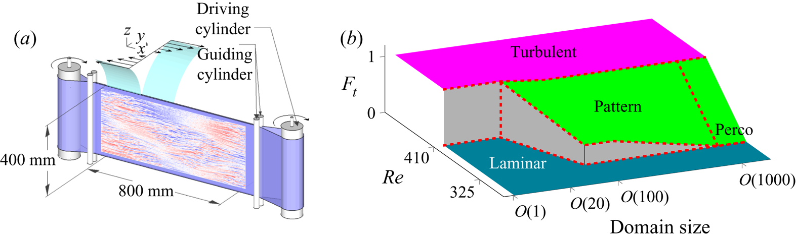
For these subcritical transitions, the natural control parameter is the Reynolds number  $Re$ and a simple and relevant order parameter is the turbulent fraction which is defined as the proportion of two-dimensional (2-D) space parallel to the walls which is turbulent. After Philip & Manneville (Reference Philip and Manneville2011), we present in figure 1(b) a sketch of the transition diagram of the plane Couette flow in which the turbulent fraction is plotted as a function of the Reynolds number and also of the aspect ratio, i.e. the size of the domain in units of the distance between the wall, which is indeed another very important control parameter. In the minimal flow unit introduced by Jimenez & Moin (Reference Jimenez and Moin1991) as the smallest domain able to maintain a turbulent state (composed of a limited number of streaks and vortices), the transition to turbulence is a purely temporal problem, the entire flow being either laminar or turbulent. When the aspect ratio is in the range of
 $10^2\text {--}10^3$ in gap width units, turbulent patches can be isolated in an otherwise laminar flow. These patches can take various forms: isolated turbulent spots, such as those initially observed in the boundary layer by Emmons & Bryson (Reference Emmons and Bryson1951) or laminar–turbulent patterns organized in oblique bands and recalling the turbulent spiral discovered by Coles (Reference Coles1962) and van Atta (Reference van Atta1966). The level of organization and the complexity of these patterns depend on the aspect ratio of the system, as shown by Duguet, Schlatter & Henningson (Reference Duguet, Schlatter and Henningson2010). In actual 2-D flows, such as plane Couette, plane Poiseuille (Tsukahara et al. Reference Tsukahara, Kawaguchi, Kawamura, Tillmark and Alfredsson2010) or plane Couette–Poiseuille (Klotz & Wesfreid Reference Klotz and Wesfreid2017) flow, large-scale flows develop around these localized turbulent zones (Lagha & Manneville Reference Lagha and Manneville2007; Duguet & Schlatter Reference Duguet and Schlatter2013; Lemoult, Aider & Wesfreid Reference Lemoult, Aider and Wesfreid2013; Couliou & Monchaux Reference Couliou and Monchaux2015; Wang et al. Reference Wang, Guet, Monchaux, Duguet and Eckhardt2020) allowing a more complex dynamic of the turbulent fraction or favouring the growth of turbulent spots as revealed by Couliou & Monchaux (Reference Couliou and Monchaux2016, Reference Couliou and Monchaux2017). On the other hand, in 1-D flows such as pipes or confined Taylor–Couette systems (Lemoult et al. Reference Lemoult, Shi, Avila, Jalikop, Avila and Hof2016), laminar–turbulence coexistence is possible but no complex dynamics is expected. For even larger aspect ratios,
 $\textit{O} (10 ^ 4)$ or more, several experiments and numerical simulations have shown that, in the vicinity of
 $Re_g$, the transition falls into the universality class of directed percolation (Lemoult et al. Reference Lemoult, Shi, Avila, Jalikop, Avila and Hof2016; Sano & Tamai Reference Sano and Tamai2016; Chantry, Tuckerman & Barkley Reference Chantry, Tuckerman and Barkley2017) as initially suggested by Pomeau (Reference Pomeau1986). The transition is therefore continuous rather than discontinuous as observed in the smaller aspect ratio systems (Bottin & Chaté Reference Bottin and Chaté1998; Bottin et al. Reference Bottin, Daviaud, Manneville and Dauchot1998; Duguet et al. Reference Duguet, Schlatter and Henningson2010).
 $(a)$ General sketch of the experimental device of plane Couette flow. A typical velocity field in the streamwise direction obtained by particle image velocimetry (PIV) is superimposed on it. The PIV field is given to scale, which shows that the PIV window fills the whole volume of the experiment.
 $(b)$ Sketch of the transition diagram as a function of
 $Re$ and of the aspect ratio. Figure inspired by Philip & Manneville (Reference Philip and Manneville2011) where the directed percolation regime has been added in the vicinity of
 $Re_g$ for very high aspect ratio systems. The order parameter in this figure is the turbulent fraction
 $F_t$ defined in almost 2-D flows as the proportion of the flow area parallel to the walls that is turbulent.

As the subcriticality of the transition implies a very strong hysteresis, the whole history of the system must be taken into account to explain the observed states. In this order of ideas, the first experimental studies of Couette flow made the distinction between the transition to turbulence (increasing  $Re$) and the transition from turbulence (decreasing
 $Re$) as in Prigent & Dauchot (Reference Prigent and Dauchot2005). The nature of the disturbance to the base flow also plays a role. After Trefethen et al. (Reference Trefethen, Trefethen, Reddy and Driscoll1993), many studies have focused on the minimum energy required to trigger the transition to turbulence, looking for scaling laws of this magnitude with
 $Re$. The first results were obtained in pipes by Darbyshire & Mullin (Reference Darbyshire and Mullin1995) while Dauchot & Daviaud (Reference Dauchot and Daviaud1995) were interested in plane Couette flow. As far as phase space is concerned, a classical description in terms of a dynamical system of the transition to turbulence in wall-bounded shear flows implies the existence of a limit in the phase space that separates the initial perturbations capable of triggering turbulence from those that will eventually decay and disappear (Itano & Toh Reference Itano and Toh2001; Skufca, Yorke & Eckhardt Reference Skufca, Yorke and Eckhardt2006). The laminar–turbulent boundary is a manifold of codimension one on which the saddle points behave as relative attractors and are called edge states. These edge states have attracted much attention over the last decade, allowing their identification in pipe flows by Schneider, Eckhardt & Yorke (Reference Schneider, Eckhardt and Yorke2007) and Willis & Kerswell (Reference Willis and Kerswell2008) and in Couette flows by Duguet, Schlatter & Henningson (Reference Duguet, Schlatter and Henningson2009). Edge states are one of the many coherent structures that develop in shear flows bounded by walls. Gibson, Halcrow & Cvitanovic (Reference Gibson, Halcrow and Cvitanovic2008) give an overview of the diversity of these structures for plane Couette flow in very small domains of the order of the minimal flow unit. Indeed, the picture is much more complicated in large domains for which the nature of the laminar–turbulent transition is different and in which the edge states are always localized.
This paper was inspired by figure 8 of Prigent & Dauchot (Reference Prigent and Dauchot2005) where the turbulent fraction is plotted as a function of time for two experiments in a plane Couette flow for which the Reynolds number was suddenly lowered from a value greater than  $Re_t$ to a value less than
 $Re_g$. Rapid fluctuations can be observed around the dynamics extending over a longer time scale. This slow dynamics takes place between two states with turbulent fractions equal to 0.15 and 0.3 respectively. The authors do not mention this dynamics while Bottin & Chaté (Reference Bottin and Chaté1998) briefly name these states metastable plateaus in the legend of their figure 6. Our curiosity is thus spurred as to their nature, their probability of occurrence and the parameters controlling their appearance. In this work, we try to answer these questions. In a complementary way, we also wonder about the existence and uniqueness of asymptotic/long-term stable states in the transitional regime where laminar and turbulent states coexist. Finally, we study the influence of forcing and history on asymptotic and transient states.
The document is organized as follows. Section 2 presents the experimental design and protocol as well as the measurement and post-processing techniques used. In § 3, dedicated to the results, we illustrate the dynamics typically observed by presenting time plots of the turbulent fraction. The asymptotic states and their dependence on the control parameters of the system are then quantified. Finally, we focus on the dynamics of the turbulent fraction which allows us to identify transient states and reveal three decay scenarios. All results are summarized and discussed in § 4.
2. Set-up and methods
This section presents the experimental set-up and protocols, the measurements and visualization systems and the different post-processing techniques applied to the data.
2.1. Experimental set-up
As sketched in figure 1, an endless 0.25 mm thick plastic belt is stretched between two cylinders. One of them is connected to a brush-less servo-motor which drives the system through a gear reducer of ratio  $9$. This motor can achieve a maximal speed of 2500 rpm. Speed and acceleration are controlled with an accuracy of
 $2/1000$. Four smaller cylinders guide the belt and continuously adjust the gap between the two walls moving in opposite directions with an accuracy of 0.05 mm. This set-up is immersed in a tank filled with water. Water temperature is monitored by a thermocouple with a
 $0.5\ ^{\circ }\textrm {C}$ accuracy. The Reynolds number is defined as
 $Re=Uh/\nu$, where
 $\nu$ is the kinematic viscosity of the fluid,
 $U$ the belt velocity and
 $h$ the half-gap between the two faces of the belt. The uncertainties on the belt velocity, the gap width and the water temperature lead to an uncertainty on
 $Re$ of
 ${\pm }2.5$. The work presented here corresponds to a gap of
 $2h=7.5\ \textrm {mm}$. The plastic belt used is very smooth, the main roughness inhomogeneity comes from the tape used to close the belt that is
 $75\ \mathrm {\mu }\textrm {m}$ thick. We have checked that no measurable waves are generated in the flow when the tape passes on the guiding cylinders. Due to the experimental geometry, a plane Couette profile is achieved within a
 $L_x=800\ \textrm {mm}$ (along
 $x$)
 $\times$
 $L_z=400\ \textrm {mm}$ (along
 $z$) area fitting our visualization field of view. The corresponding aspect ratios are thus
 $\varGamma _x=L_x/h=214$ and
 $\varGamma _z=L_z/h=107$;
 $x$,
 $y$ and
 $z$ and
 $U_x$,
 $U_y$ and
 $U_z$ are respectively the streamwise, wall-normal and spanwise directions and the associated velocities. The plane
 $y=0$ is located at half the distance between the two plates. The tank is closed at the top by a transparent Plexiglas lid wherever the plane Couette profile is achieved in order to enable top and bottom symmetrical boundary conditions. We have checked the temperature homogeneity in the flow and the absence of thermal convection effects. A recirculating pump used between experimental sessions allows us to get rid of the bubbles naturally forming in still water. From various experiments not detailed here, critical Reynolds numbers have been obtained as
 $Re_g\simeq 320$ and
 $Re_t \simeq 400$, consistently with previous experiments and well-resolved direct numerical simulations Bottin et al. (Reference Bottin, Daviaud, Manneville and Dauchot1998); Duguet et al. (Reference Duguet, Schlatter and Henningson2010).
2.2. Particle image velocimetry measurements and visualizations
Velocity measurements have been carried out by PIV over the entire area where plane Couette flow exists. To do this, the flow is illuminated by a laser diode combined with a high-frequency rotating polygonal mirror to produce a laser sheet that illuminates the flow along the median plane located in  $y=0$. The flow is seeded with Rhodamine coated particles with a diameter
 $d_p\text { of} =1\text {--}20\ \mathrm {\mu }\textrm {m}$ which scatter light at a shifted wavelength. A filter mounted on the camera lens is used to keep only the wavelengths around this shifted wavelength, thus getting rid of unwanted light reflections on the plastic container and belt. Images at a resolution of approximately
 $2050\times 1025\ \textrm {pixels}^{2}$ corresponding to an observation window of
 $800\times 400\ \textrm {mm}^{2}$ – exactly matching the area where the laminar Couette profile is achieved – are captured at 20 Hz by a PCO sCMOS Camera provided by PhotonLine. In figure 1(a) a typical PIV field with both laminar and turbulent phases coexisting has been superimposed on the facility sketch to illustrate this exact matching. The PIV calculations are performed between consecutive images using a code based on an optical flow technique and presented in Quénot, Pakleza & Kowalewski (Reference Quénot, Pakleza and Kowalewski1998). The main advantage of this code is to provide high accuracy PIV at high resolution: a velocity vector is obtained for every pixel in the image. The result is a spatial resolution of 0.39 mm, i.e. 0.104 h. Thanks to this high resolution, it is possible to perform robust calculations of derived quantities such as the normal wall vorticity. To limit the computation time, the velocity fields are actually calculated at an effective sampling rate of 1 or 4 Hz depending on the individual experiments. The time signals presented in this article are therefore displayed at different sampling rates. Each instantaneous velocity field is then filtered by eliminating values greater than 1.2
 $U$. The resulting outliers are replaced by local median filters.
2.3. Experimental protocol
In the context of transition from turbulence, the system can be prepared at an initial value  $Re_i$ greater than
 $Re_t$, then the Reynolds number is reduced to a final value
 $Re_f$ within
 $[Re_g,Re_t]$. Again, the system will evolve to a state that may depend on
 $Re_f$ and also on the rate at which it has been reached. In almost all former studies, the Reynolds number was suddenly reduced from
 $Re_i$ to
 $Re_f$ (Bottin et al. Reference Bottin, Daviaud, Manneville and Dauchot1998; Peixinho & Mullin Reference Peixinho and Mullin2006) and we will call these experiments ‘quenches’. Following the idea of Schmiegel & Eckhardt (Reference Schmiegel and Eckhardt2000), we carry out annealing experiments, that is to say slow continuous decreases of the Reynolds number from
 $Re_i$ to
 $Re_f$ at a rate of
 $\dot {Re}$ unit per second. Therefore, in any experiment, the current Reynolds number is
 \begin{gather} Re(t)=Re_i-t\dot{Re},\quad \mathrm{for}\ t\leq t_f, \end{gather}
 \begin{gather} Re(t)=Re_f, \quad \mathrm{for} \ t\geq t_f, \end{gather}
with  $t_f=({Re_i-Re_f})/{\dot {Re}}$ the time at which the final Reynolds number is reached.
Since our purpose is to explore the possible asymptotic states in the coexistence region as well as the relaxation dynamics of the system in this same region, we choose  $Re_f$ in the range
 $[300,410]$;
 $Re_i$ is always set to
 $430$;
 $\dot {Re}$ is fixed to
 $0.3$,
 $1$ or
 $5\ \textrm {s}^{-1}$, corresponding to
 $0.0098$,
 $0.0325$ and
 $0.163$ in units of
 $h/U_i$,
 $U_i$ being the velocity of the initial value
 $Re_i$ at
 $20\ ^{\circ }\textrm {C}$. In order to compare with former studies, we also perform quenches by suddenly decreasing
 $Re$ from
 $Re_i$ to
 $Re_f$ within less than 0.3 s, i.e. always less than 5 advective time units based on initial velocity. To ensure reproducibility, the system is prepared at
 $Re_i$ and held there for at least 2 min to reach a fully turbulent state, then
 $Re$ is decreased. Time
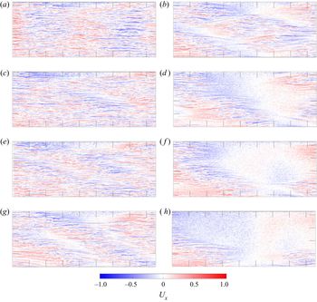
 $t=0$ corresponds to the initiation of quenching or annealing. Figure 2 shows a typical annealing between
 $Re_i=430$ and
 $Re_f=340$ at
 $\dot {Re}=0.3\ \textrm {s}^{-1}$.
Succession of snapshots of the streamwise velocity  $U_x$ along a typical annealing from
 $Re_i=430$ to
 $Re_f=300$ at a rate
 $\dot {Re}=0.3\ \textrm {s}^{-1}$. Time is given in units of
 $h/U_i$. Colour bars are identical for all velocity contour plots in this article. Ticks are equispaced by 25 units of
 $h$.
 $(a) \ t = 0, \ (b) \ t = 6500\,h/U, \ (c) \ t = 2600\,h/U, \ (d) \ t = 9100\,h/U,$
 $(e) \ t = 3900\,h/U, \ (\,f) \ t = 10\,400\,h/U, \ (g) \ t = 5200\,h/U \ {\rm and}$
 $(h) \ t = 11\,700\,h/U$.

2.4. Post-processing
The turbulent fraction  $F_t$, defined in
 $(x,z)$ planes as the ratio of turbulent flow area to total flow area, is calculated from the in-plane velocity rather than from visualizations from platelets as in most experimental facilities of transitional turbulence. From the
 $(u_x,u_z)$ velocity field,
 $\omega _y$, the wall-normal vorticity is calculated using the PIVmat toolbox function vec2scal with option rot (Moisy Reference Moisy2020). Due to the very high spatial resolution available here, the calculated vorticity fields are reasonably smooth. They are further binarized to provide a raw estimation of the turbulent regions as areas where
 $|\omega _y|>0.205$ in dimensionless units. A succession of opening/closure with structuring elements diamonds/disks is thus applied to close gaps between streaks and to remove tiny areas mistakenly identified as turbulent because of derivation noise. This is a specific use of mathematical morphology (Haralick, Sternberg & Zhuang Reference Haralick, Sternberg and Zhuang1987). A sensitivity analysis of the thresholds and parameters used was performed and a thorough visual calibration of the detection quality was carried out to adjust the parameters and ensure the reproducibility and robustness of the segmentation procedure. The results presented here are obtained from the temporal evolution of the turbulent fraction. We also studied the temporal evolution of the total kinetic energy in the measurement plane, which leads to almost identical plots as already reported by Manneville (Reference Manneville2011).
3. Results
3.1. Typical dynamics
The succession of snapshots shown in figure 2 represents a typical annealing between  $Re_i=430$ and
 $Re_f=300$ at
 $\dot {Re}=0.3\ \textrm {s}^{-1}$. It is visualized from streamwise velocity fields. The dynamics is as follows. Laminar holes open up while the turbulent intensity in the turbulent zones remains almost at the same level. Indeed, the spatial density of turbulent kinetic energy, i.e. the kinetic energy within turbulent patches divided by their total area, is a slowly decreasing function of the Reynolds number (not shown), as already reported by Manneville (Reference Manneville2011) in his figure 9, for example. Later on, the holes get larger and eventually organize into oblique stripes typical of extended internal shear flows. When the turbulent fraction is too low to maintain a band, isolated turbulent spots remain and slowly disappear by fading away due to viscosity rather than by receding spatially.
3.2. Time traces
From now on, the turbulent fraction  $F_t$ will be used as a single scalar parameter to follow the annealing dynamics. This is obviously restrictive but allows us, nevertheless, to gain a relevant insight into the studied system. Given our system, time can be made non-dimensional in different ways. For experiments or simulation performed at given
 $Re$, i.e. at given belt velocity
 $U$, one can built an advective time unit
 $h/U$ and a diffusive time unit
 $h^2/\nu$, the former being more relevant to the kind of dynamics we are interested in. Since the advective time scale depends on
 $U$, it is evolving with time and we have thus chosen to rescale time using
 $\dot {Re}$, which has the correct dimension to do so, which is constant through the whole experiment and, as we will see, provides a good scaling of the control parameter. For the same reasons, the values of
 $\dot {Re}$ are given in
 $\textrm {s}^{-1}$ rather than in dimensionless units.
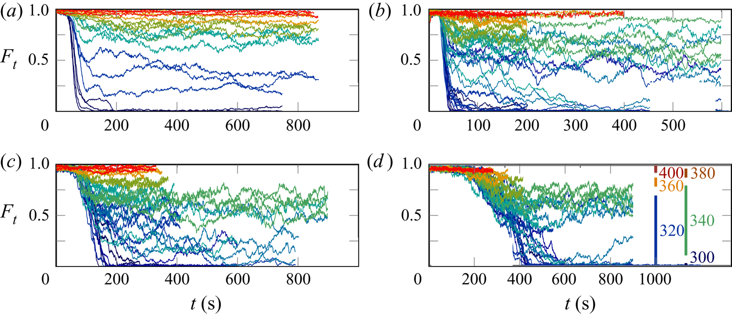
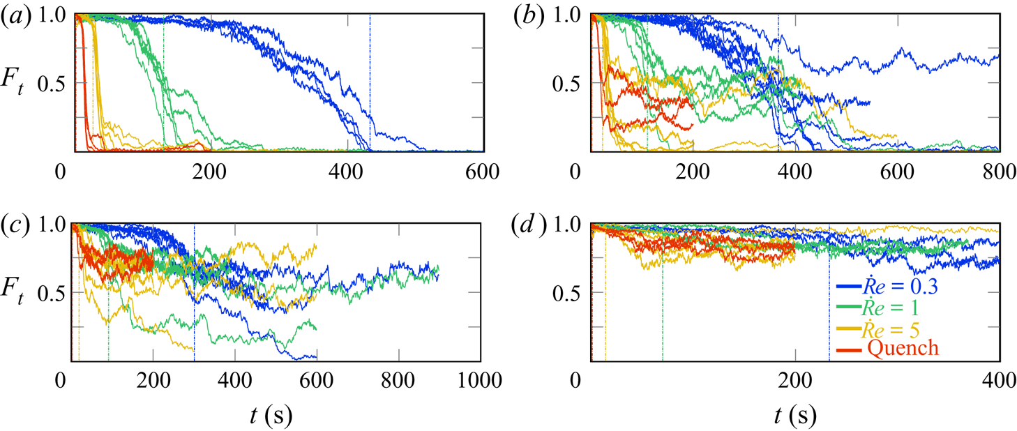
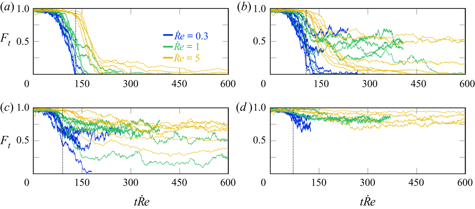
Figures 3–5 present the time evolution of the turbulent fraction. To improve readability, only a subset of the studied  $Re_f$ are displayed. Nevertheless, figure 6 and our comments gather all our observations. In figures 4 and 5, time traces are coloured according to the value of
 $\dot {Re}$ and gathered in the same panel by
 $Re_f$ values while in figure 3 it is the opposite. In these figures, time is given either in seconds or in units of
 $\dot {Re}$.
Turbulent fraction versus time for all  $Re_f$ for four different
 $\dot {Re}$ values. Final Reynolds numbers
 $Re_f$ are indicated in
 $(d)$. Traces with the same colour correspond to various experiments performed with the same parameters. In panel
 $(d)$, the bars labelled with values of
 $Re_f$ indicate the span of
 $F_t$ values reached asymptotically between different realizations with the same parameters. See figure 6 for a more quantitative picture.
 $(a) \ {\rm Quench}, \ (b) \ \dot{R}e = 5, \ (c)\ \dot{R}e = 1 \ {\rm and} \ (d) \ \dot{R}e = 0.3.$

Turbulent fraction versus time for all  $\dot {Re}$ for four different
 $Re_f$ values. Traces with the same colour correspond to various experiments performed with the same parameters. Vertical dash-dotted lines indicate
 $t_f$, the time at which the final Reynolds number
 $Re_f$ is reached. For quenches, this line is sometimes hidden by the ordinate axis.
 $(a) \ \textit{Re}_{f} = 300, \ (b) \ \textit{Re}_{f} = 320, \ (c) \ \textit{Re}_{f} = 340 \ {\rm and} \ (d) \ \textit{Re}_{f} = 360.$

Turbulent fraction versus rescaled time  $t\dot {Re}$ for all
 $\dot {Re}$ for four different
 $Re_f$ values. Traces with the same colour correspond to various experiments performed with the same parameters. Vertical dash-dotted lines indicate
 $t_f$, the time at which the final Reynolds number
 $Re_f$ is reached. Note that with this scaling they occur at the same
 $t\dot {Re}$ value for all experiments performed at the same
 $Re_f$, regardless of
 $\dot {Re}$ value. Quenches are not presented here because, due to our experimental protocol, the time rescaling used here is not relevant for quenches.
 $(a) \ \textit{Re}_{f} = 300, \ (b) \ \textit{Re}_{f} = 320, \ (c) \ \textit{Re}_{f} = 340 \ {\rm and} \ (d) \ \textit{Re}_{f} = 360.$

All together, these figures show that the turbulent fraction is globally decreasing from  $F_t=1$ at
 $t=0$ toward lower values when
 $t$ increases. Regardless of
 $\dot {Re}$, when the final Reynolds number
 $Re_f$ is larger than 350 the dynamics is a trivial decay to asymptotic values, occurring with little fluctuation. For
 $Re_f=300$, the decay to
 $F_t=0$ is also fairly simple and with little fluctuation, but for decay rates
 $\dot {Re} \geq 1\ \textrm {s}^{-1}$, transient plateaus are often seen, as has already been observed by Prigent & Dauchot (Reference Prigent and Dauchot2005). The following sections provide a statistical analysis of these results.
The time at which the final Reynolds number  $Re_f$ is reached is denoted in figures 4 and 5 with vertical dash-dotted lines. Interestingly, transient plateaus are seen when the system has already reached a Reynolds number value for which the asymptotic turbulent fraction is lower than that of the visited plateau. When rescaling time with
 $\dot {Re}$, as in figure 5, the final Reynolds number
 $Re_f$ is reached at
 $t\dot {Re}=Re_i-Re_f$, regardless of the value of
 $\dot {Re}$. The
 $F_t(t)$ curves associated with different
 $\dot {Re}$ get closer to each other when plotted against
 $t\dot {Re}$ but do not completely collapse. However, the order of the plots is reversed when comparing figure 4 with figure 5. When
 $F_t$ is plotted versus the non-dimensional time
 $t\dot {Re}$, it appears that, with this time scale, the dynamics is faster for lower
 $\dot {Re}$ or delayed for larger decay rate. This will be further discussed in the next section when commenting on the results from figure 8.
3.3. Asymptotic states
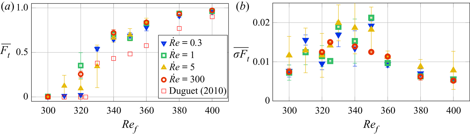
Figure 6(a) presents the  $Re_f$ dependence of
 $\overline {F_t}$, the time average of the turbulent fraction calculated over the asymptotic plateaus described in the previous paragraph. Numerical simulation data from Duguet et al. (Reference Duguet, Schlatter and Henningson2010) were added for comparison; they have been obtained from the asymptotic state reached when a localized perturbation is added to the laminar flow. To quantify the level of fluctuations around the dynamics, we have calculated
 $\sigma _{F_t}$, the moving standard deviation of the turbulent fraction over time intervals of
 $T=15\ \textrm {s}$, as
 \begin{equation} \sigma_{F_t}(t) = \sqrt{\frac{1}{T}\int_{t-T/2}^{t+T/2}F_t^2(t')\,\textrm{d}t' - \left(\frac{1}{T}\int_{t-T/2}^{t+T/2}F_t(t')\,\textrm{d}t'\right)^2}. \end{equation}
 $(a)$ Asymptotic turbulent fraction
 $\overline {F_t}$ as a function of
 $Re_f$ for various
 $\dot {Re}$. Error bars represent the dispersion between experiments performed with the same control parameter values. Data from Duguet et al. (Reference Duguet, Schlatter and Henningson2010) are also presented.
 $(b)$ Time average of the moving standard deviation calculated over time intervals of 15 s. This quantity measures the level of fluctuations around the smoothed dynamics.

Figure 6(b) presents  $\overline {\sigma _{F_t}}$, the time average of this moving standard deviation versus
 $Re_f$;
 $\overline {F_t}$ has an expected behaviour – it grows from zero at
 $Re_f\leq Re_g$ to one when
 $Re_f\geq Re_t$. The dispersion between similar experiments is very low, often less than the size of the symbol. For most values of
 $Re_f$ (when
 $Re_f$ is not in the range 310–330) we do not see any dependency of the results on
 $\dot {Re}$, indicating that, as far as annealing and quenches are concerned, the average asymptotic turbulent fraction does not depend on the specific history of the system. Numerical values obtained by Duguet et al. (Reference Duguet, Schlatter and Henningson2010) are systematically lower than ours which could be due to either the different protocol (transition from versus transition to turbulence) or the domain size, which is four times larger in the numerical simulations. In the range
 $310\leq Re_f\leq 330$, a large variability of the results is observed, as expected in the vicinity of a critical point. Figure 6(b), presenting the average level of fluctuations around the moving average state, shows that these inner fluctuations present a maximum for
 $Re_f \simeq 330\text {--}350$, which indeed corresponds to a range where large-scale flows have larger amplitudes, see Couliou & Monchaux (Reference Couliou and Monchaux2015). We thus interpret these low-frequency fluctuations as slow reorganizations of the turbulent regions involving strong secondary flows.
3.4. Turbulent fraction dynamics
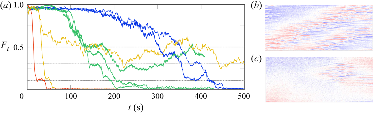
Figure 7 presents some trajectories selected from figure 4 for all available  $\dot {Re}$ values at
 $Re_f=300$ (continuous lines) and
 $Re_f=320$ (dash-dotted lines). We have chosen them to illustrate the turbulent fraction dynamics slowing down on the transient plateaus introduced in the previous section. Three well-defined plateaus can be identified: one around
 $F_t=0.5$, one around
 $F_t=0.3$ and one around
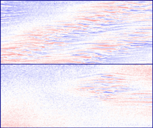
 $F_t=0.1$. We systematically observed the topology of the velocity fields associated with these plateaus and found that they correspond respectively to two bands, one band and a minimal spot, as shown in figure 7(c,d). Minimal spots will be clearly defined in § 3.5. Statistically, from more than 200 studied experiments, it appears that approximately
 $50\,\%$ of the trajectories that can visit these states, i.e. trajectories whose asymptotic state is below
 $F_t=0.5$, actually visit them. Surprisingly, the turbulent fraction dynamics is not monotonic, even if the controlling Reynolds number dynamics is. More surprisingly, most of the complex and non-monotonic dynamics takes place when the current Reynolds number is already equal to
 $Re_f$, i.e. to the right of the vertical dash-dotted lines of figures 4 and 5. Note that this remains true even when the final Reynolds number is below the global stability threshold
 $Re_g$. Consider, for example, the green trajectories in figure 7 that have been performed at
 $\dot {Re}=1$ and
 $Re_f=300$ or
 $Re_f=320$: in both cases, at
 $t=110\ \textrm {s}$, the final Reynolds number is reached and the expected state is
 $F_t=0$. Instead, we see that the system either stays on transient plateaus until much later times at approximately
 $t=200\ \textrm {s}$ or, for
 $Re_f=320$, develops long-term fluctuations between transient plateaus at times exceeding the experiment duration (400 s or even 600 s). These observations raise many questions about the nature of these states and in particular about their topology in the phase space. They also reveal the influence of the
 $\dot {Re}$ decay rate on the dynamics and highlight the great difference between quench and annealing. Indeed, transient plateaus are not observed for the lowest decay rates for which the dynamics almost follows the asymptotic
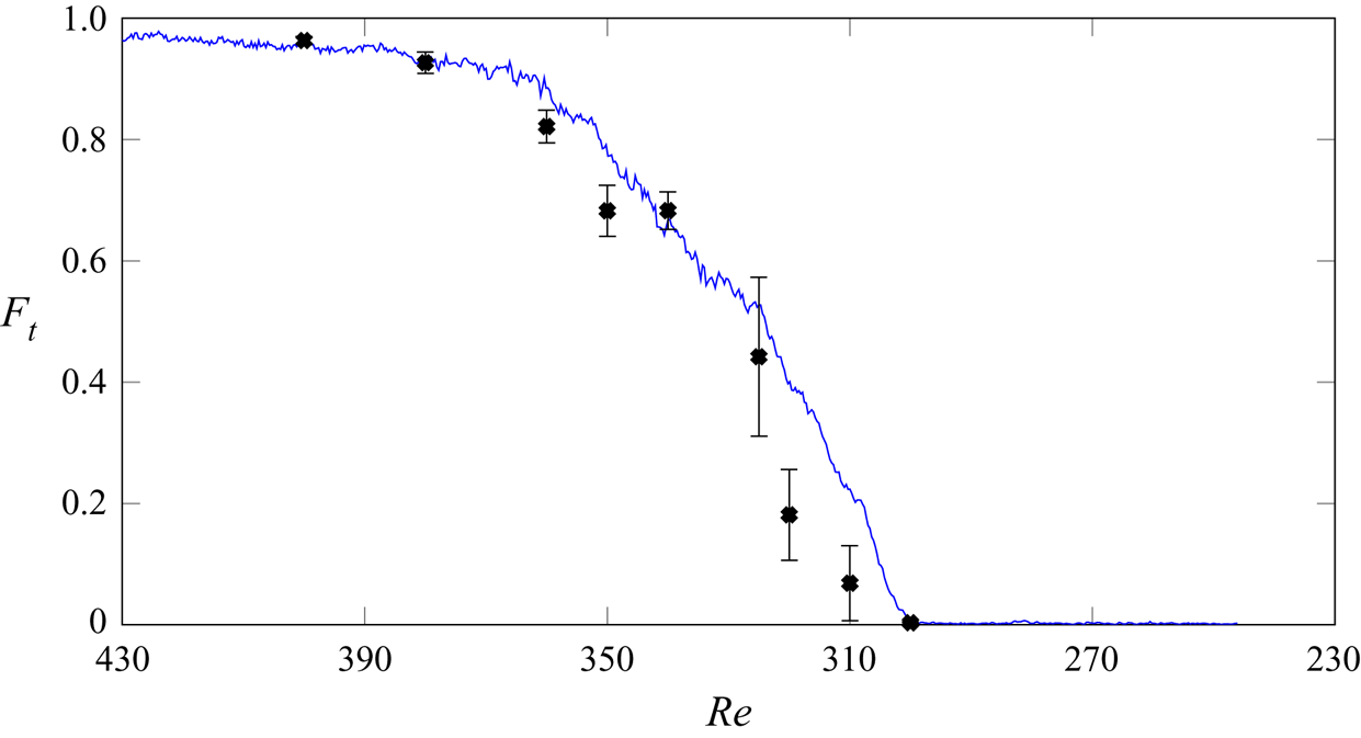
 $F_t(Re)$ curve, as can be seen in figure 8 where the asymptotic data of figure 6 are plotted together with the dynamic data of figure 5. This simultaneous plotting is possible because, when the time is scaled with
 $\dot {Re}$,
 $Re_i - t\dot {Re}$ is the current Reynolds number. We can see that the two curves collapse on top of each other, except perhaps for the larger
 $Re$ for which the dynamics is still delayed with respect to the evolution of the control parameter. A better collapse should be achieved by an even slower annealing at a lower
 $\dot {Re}$.
(a) Some particular turbulent fraction dynamics picked up to illustrate the robustness of the plateaus. Traces are coloured according to  $\dot {Re}$ as in figure 4, continuous lines are for
 $Re_f=300$, dash-dotted lines for
 $Re_f=320$. (b,c) Typical velocity fields associated with turbulent fraction plateau at
 $F_t\simeq 0.5$ (b) and
 $F_t\simeq 0.1$ (c). They respectively correspond to experiments performed at
 $\dot {Re}=0.3$ and
 $\dot {Re}=1$ for a common
 $Re_f=300$.

Turbulent fraction versus Reynolds number. The continuous blue line is the ensemble average of data from figure 5 obtained for  $Re_f=300$ and
 $\dot {Re}=0.1$, in this case
 $Re$ is the current Reynolds number. Black symbols with error bar are the ensemble average and standard deviation of data displayed in figure 6, in this case
 $Re$ is the final Reynolds number. See text for details.

3.5. Phase portrait
Trying to gain insight into the nature of the transient states and of the trajectories visiting them in the phase space, we have intended to draw phase portraits from first return maps to represent the transient trajectories discussed here. The most natural idea was to focus only on  $F_t$ and we thus started by plotting
 $F_t(t)$ versus
 $F_t(t+\Delta t)$ for various time increments
 $\Delta t$. If this method is suitable for simple low-dimensional dynamical systems, it may be more difficult to use it to get relevant information in our spatially extended case. We have thus introduced other global physical quantities linked to spatial inhomogeneities of the flow. Due to the complex spatio-temporal nature and the high dimensionality of the studied system, no obvious reconstruction leading to insightful interpretation of the results could be obtained to better understand the nature of the transient states. Nevertheless, the outcomes of this work, that we will present as phase portraits, have allowed us to identify different turbulence retreat scenarios.
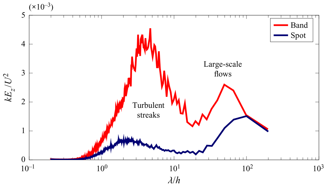
From our full resolution PIV system and 2-D power spectrum calculations, we have access to the power spectral density for wavelengths between 0.2 and 200 in dimensionless units. Examples of such instantaneous spectra obtained for an isolated band and a spot are presented in figure 9. From  $1.6h$ to
 $10h$ the energy content is associated with streaks and corresponds to turbulent areas. Then, a spectral gap is observed around
 $\lambda _c\simeq 20h$. Above, from
 $30h$ to
 $100h$, the spectral content corresponds to large-scale flows. See Couliou & Monchaux (Reference Couliou and Monchaux2015) for a similar discussion from narrower PIV fields. By integrating the whole large-scale flow energy content, we have a measure of the large-scale flow intensity
 $A_{LSF}$ that is obtained as follows. We first calculate the instantaneous
 $u_z$ 2-D premultiplied power spectral density
 $S_{u_z}$ as
 \begin{equation} S_{u_z}(k_x,k_z,t) =|k|\times |\hat{u}_z(k_x,k_z,t)|^2, \end{equation}
where  $\hat {u}_z(k_x,k_z)$ is the instantaneous two-dimensional Fourier transform of
 $u_z$ and
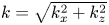 $k=\sqrt {k_x^2+k_z^2}$. Then, we integrate the premultiplied spectrum along the azimuthal direction as
 \begin{equation} E_z (k,t)= \frac{1}{2{\rm \pi}}\int_0^{2{\rm \pi}}S_{u_z}(k_x,k_z,t)\,\textrm{d}\theta, \end{equation}
with  $\theta =\arctan (k_z/k_x)$. Finally, integration over the large-scale wavelength yields an estimation of the large-scale flow intensity as
 \begin{equation} A_{LSF}(t) = \int_{\lambda/h=30}^{\lambda/h=100}kE_z(k,t)/U^2\,\textrm{d}k, \end{equation}
where  $k=2{\rm \pi} /\lambda$.
Typical power spectral density of  $u_z$ averaged azimuthally for a flow containing bands (as in figure 7b) or a spot (as in figure 7c). They respectively correspond to experiments performed at
 $\dot {Re}=0.3$ and
 $\dot {Re}=1$ for a common
 $Re_f=300$. Turbulent streaks produce a rise in energy in a band of
 $\lambda /h\in [10^0\text {--}10^1]$ while large-scale flows produce energy for
 $\lambda /h\in [3\times 10^1\text {--}2\times 10^2]$.

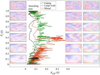
Phase portraits for each experiment have been obtained by plotting  $F_t(t)$ versus
 $A_{LSF}(t)$. The systematic observation of all the phase portraits has led to the identification of three types of trajectories exemplified in figure 10. Some trajectories go from
 $F_t=1$ toward
 $F_t=0$ with few fluctuations and without developing any large-scale flow while others quickly develop large-scale flows. These last much longer and have a much more complex dynamics. Finally, hybrid trajectories exist that start on the quick path but start to develop large-scale flow at some point and end on the complex and long lasting path. Figure 10 also presents snapshots of the streamwise velocity field taken along these three types of trajectories. Comparing them to each other, it appears that the same levels of turbulent fraction in both cases do not correspond to the same physical state at all. On the large-scale path, the turbulent part of the velocity field is actually made of intense, well defined and instable streaks while on the fast path we observe smooth spatial velocity fluctuations organized as streaks resembling what can be observed in the laminar wake of an object placed in a shear flow or around a localized turbulent spot, see, for example, Couliou & Monchaux (Reference Couliou and Monchaux2016) or Couliou & Monchaux (Reference Couliou and Monchaux2017). These two behaviours actually correspond to two ways in which turbulence declines. In the first case, when laminar holes appear, turbulence (i.e. streaks) intensity remains the same in the turbulent regions whose area progressively diminishes. Thus, turbulence recedes in area but not in intensity. In the second case the emergence of laminar holes goes along with a diminution of the turbulent intensity within turbulent regions and turbulence decreases more in intensity than in area. We thus call these trajectories fading ones. Interestingly, even on large-scale paths, when only a turbulent spot is left, it disappears as it fades, the turbulence losing intensity without decreasing in area. This shows that the imposed shear cannot maintain a turbulent spot which is smaller than a given size. We thus refer to these spots of minimal size as minimal spots. An example of such a minimal spot can be found in figure 7.
Phase portrait presenting three representative trajectories in the plane ( $F_t(t),A_{LSF}(t)$). Snapshots along these three paths are also shown to illustrate the differences between them. From top to bottom, turbulent fraction is 1, 0.9, 0.7, 0.5, 03 and 0.1. Panel frames are coloured according to the followed path.

4. Discussion and conclusion
In this article, we have investigated the dynamics of turbulence retreat in plane Couette flow when the Reynolds number is decreased. We studied the influence of a rate of decrease in Reynolds number,  $\dot {Re}$ and its final value
 $Re_f$. To do so, we have spanned a large range in parameter space going from very sudden decreases of
 $Re$ (quenches) to much smoother decreases (annealing). We have shown that the long-term (asymptotic) turbulent fraction decreases when decreasing
 $Re$, converging to plateaus that are well defined when
 $Re_f$ is high enough above
 $Re_g$. In contrast, when
 $Re_f$ is close to
 $Re_g$, strong fluctuations are observed that delay the stabilization around the asymptotic state, as expected near a critical point. If the asymptotic states depend only on
 $Re_f$, the retreat dynamics strongly depends on
 $\dot {Re}$. If
 $\dot {Re}$ is sufficiently low to allow the system to always be at equilibrium, the time series of the turbulent fraction
 $F_t(t)$ follow the asymptotic curve
 $F_t(Re(t))$, with
 $Re(t)=Re_i-t\dot {Re}$. This is almost done in figure 8. When
 $\dot {Re}$ is larger, the system cannot relax fast enough to always be at equilibrium and the retreat dynamics lags behind the decreasing control parameter. As a consequence, before the final Reynolds number
 $Re_f$ is reached, the instantaneous turbulent fraction
 $F_t(t)$ is always higher than its expected asymptotic value
 $F_t(Re(t))$ at the current value of the Reynolds number
 $Re(t)$. After a time
 $t=t_f$, when the final Reynolds number is reached, i.e. beyond the vertical dash-dotted lines of figures 4 and 5, the dynamics can be interpreted as follows. As the phase space only depends on
 $Re_f$, it does not change over time. The state of the system at
 $t=t_f$ can thus be considered as an initial condition that will relax to its asymptotic state. On this path, the system visits the transient plateaus described in § 3.4. These specific states are laminar–turbulent alternating stripes or isolated turbulent spots. A striking feature we observed is that turbulent fraction may stay at a high level or even increase in spite of the fact that the Reynolds number has already decreased below the critical value at which turbulence is supposed to maintain itself. This observation should be linked to those of Schmiegel & Eckhardt (Reference Schmiegel and Eckhardt2000) in their numerical study of annealing, even if they could not see the associated complex dynamics since they were working in a very narrow system, close to the minimal flow unit. The complex dynamics of minimal spots associated with the lower transient plateau in figure 7 has already been observed in numerical simulations, as briefly described in Duguet et al. (Reference Duguet, Schlatter and Henningson2010).
The study of a section of phase space helped us to show that at least two types of turbulent retreat trajectories exist, one associated with a complex recession of turbulence favoured by the development of large-scale flows while, in the other, the turbulence only fades. The latter scenario is presumably dominated by viscosity. The present study resembles the numerical work presented in Manneville (Reference Manneville2011) and Manneville (Reference Manneville2012) in domains that could also accommodate two bands. We also observe the more or less linear decay stage of the turbulent fraction when one band decays monotonically, but the numerical work has only a transient plateau and does not study it systematically as we have done since they are interested in other statistical aspects of the retreat. For the same reason, they do not account for the non-monotonic dynamics, except for that of a tiny turbulent seed. We cannot compare this with the complex non-monotonic dynamics between minimal spots and bands presented here.
The observed transient states may be linked to particular topological states in phase space such as, for instance, edge states. Nevertheless, the long lifetime of the system on these transient plateaus rather incites us to link the observed dynamics to entangled networks of finite-amplitude solutions involving localized edge states (Duguet et al. Reference Duguet, Schlatter and Henningson2009) or other unstable solutions similar to our minimal spot (Brand & Gibson Reference Brand and Gibson2014) or to our single isolated band (Reetz, Kreilos & Schneider Reference Reetz, Kreilos and Schneider2019). Budanur & Hof (Reference Budanur and Hof2017) recently found long lived heteroclinic connections between localized periodic orbits in pipe flow. Edge states in pipe flow were observed in decaying experiments quite similar to ours by De Lozar et al. (Reference De Lozar, Mellibovsky, Avila and Hof2012) where PIV snapshots are compared to instantaneous direct numerical simulation results. Resemblance between numerically computed edge states and flow fields is calculated based on the three components in a plane. This makes it possible to decide whether an edge state is visited or not. It appears that the decaying pipe spends  $17\,\%$ of its time close to the edge state. Performing this type of tests would require the introduction of measured velocity fields in edge state tracking algorithms which may require 3-D velocity field measurements. A complementary numerical study would be very useful in this respect as the results obtained here should be readily available numerically, although the computational times required for such long-term dynamics would probably not allow the type of statistical analysis presented here.
The long lifetimes of the statistically frequent transient plateaus we have reported show the robustness of the corresponding localized solutions (minimal spots, bands) in phase space. Irrespective of the system dimension, recent observations of directed percolation and/or continuous transition to turbulence in wall-bounded shear flows has only been possible in extremely large domains. Note that this transition is continuous but what is considered as the excited state is actually a laminar–turbulent pattern. The elementary block for the continuous directed percolation transition are thus the localized bands presented in figure 7. The large-scale flows developing around them probably play an important role in stabilizing them, allowing them to persist for an arbitrary long period of time. The mechanisms responsible for their origin and localization in physical space are unfortunately still unknown despite decades of effort devoted to their study, as recently reviewed by Tuckerman, Chantry & Barkley (Reference Tuckerman, Chantry and Barkley2020).
Acknowledgements
We are grateful to Y. Duguet and to J. Rolland for their constructive remarks on the paper and to L. Pastur and G. Lemoult for fruitful discussions. We are also very grateful with the three anonymous referees that helped us to really improve this article. This work has benefited from the ANR funding Jeunes Chercheurs/Jeunes Chercheuses QANCOUET.
Declaration of interests
The authors report no conflict of interest.