1 Introduction
Traditional explorations on the aerodynamics of an airfoil mainly focus on the high-Reynolds-number cases (the chord length Reynolds number
 $Re_{c}$
is approximately
 $10^{6}{-}10^{7}$
). In this
 $Re_{c}$
regime, the maximum lift-to-drag ratio depends weakly on
 $Re_{c}$
(Lissaman Reference Lissaman1983). Transition occurs prior to separation to form an attached turbulent boundary layer upon the airfoil. The stall of the airfoil generally results from the separation of the turbulent boundary layer (Wang et al.
Reference Wang, Zhou, Alam and Yang2014). In recent years, the low-Reynolds-number airfoils have been widely investigated driven by the demands of small aerial vehicles (Mueller & Delaurier Reference Mueller and Delaurier2003). Due to the scale effect (Lissaman Reference Lissaman1983; Haines Reference Haines1994), the aerodynamic performance of a few airfoils (single element) with good performance at high Reynolds number could seriously deteriorate at low Reynolds number (
 $Re_{c}$
smaller than
 $5\times 10^{5}$
). The separation of the laminar boundary layer contributes to the deteriorated aerodynamic performance at low Reynolds number (Boutilier & Yarusevych Reference Boutilier and Yarusevych2012a
). The transition of the separated boundary layer could finally result in the occurrence of reattachment. This reattachment forms the classical flow structure named the laminar separation bubble (Gaster Reference Gaster1969). The burst of the separation bubble results in the stall and the poor aerodynamic performance of the airfoil (Carmichael Reference Carmichael1981). Investigations on the transition processes of the laminar separation bubbles could facilitate the comprehension on the flow physics of low-Reynolds-number airfoils.
The initial transition processes of the separation bubbles have been investigated extensively. Watmuff (Reference Watmuff1999) showed that the Kelvin–Helmholtz (K–H) instability dominates the initial transition process and finally generates the shed vortex. Hain, Kähler & Radespiel (Reference Hain, Kähler and Radespiel2009) highlighted that the K–H instability of the separated shear layer is triggered by the amplified Tollmien–Schlichting (TS) wave originating from the attached boundary layer (
 $Re_{c}=6.6\times 10^{4}$
). The unsteady disturbances in the free-stream flow could perturb the amplitude of the TS wave and finally result in the flapping of the separated shear layer. Simoni et al. (Reference Simoni, Ubaldi, Zunino, Lengani and Bertini2012) showed that the modal growth associated with the K–H instability occurred after the saturation of the amplification of low frequency disturbances (flat plate length Reynolds number
 $Re_{l}$
was
 $7\times 10^{4}{-}2\times 10^{5}$
). The low frequency disturbances might also contribute to the flapping of the separated shear layer. Lang, Rist & Wagner (Reference Lang, Rist and Wagner2004) utilized a TS wave superimposed with steady three-dimensional disturbances to explore the effect of three-dimensional disturbances on the transition process of the separated shear layer (global Reynolds number
 $Re_{g}=1\times 10^{5}$
). It was found that the amplification of the two-dimensional disturbances, rather than the three-dimensional disturbances, dominated the initial transition process of the separated shear layer. Mcauliffe & Yaras (Reference Mcauliffe and Yaras2009) showed that the free-stream turbulence intensity (
 $T_{u}$
) could influence the transition process of the separated shear layer (
 $Re_{l}=3.9\times 10^{5}{-}4.4\times 10^{5}$
). Under low free-stream turbulence (
 $T_{u}=0.1\,\%$
), the K–H instability dominates the transition process of the separated shear layer. While under elevated free-stream turbulence (
 $T_{u}=1.45\,\%$
), streaky structures occur within the separated shear layer and bypass the modal growth associated with the K–H instability.
The breakdown of the shed vortex originating from the instability of the separated shear layer could facilitate the reattachment of the separated shear layer. The transition processes associated with this phenomenon are still open issues. Burgmann & Schröder (Reference Burgmann and Schröder2008) observed that the shed vortex suffers from a rapid three-dimensional deformation to form the c-shape vortex (
 $Re_{c}=2\times 10^{4}{-}6\times 10^{4}$
). The c-shape vortex evolves into screwdriver vortex pairs and finally undergoes vortex breakdown. Jones, Sandberg & Sandham (Reference Jones, Sandberg and Sandham2008) captured streamwise vortices in the braid region between two successive shed vortices
 $(Re_{c}=5\times 10^{4})$
. These streamwise vortices are similar to the braid vortices in bluff-body wakes (Williamson Reference Williamson1996). These flow structures were also captured in the experimental investigation of Kurelek, Lambert & Yarusevych (Reference Kurelek, Lambert and Yarusevych2016)
 $(Re_{c}=1\times 10^{5})$
. Marxen, Lang & Rist (Reference Marxen, Lang and Rist2013) showed that these streamwise vortices originate from the hyperbolic instability of the shed vortices
 $(Re_{g}=1\times 10^{5})$
.
It can be seen that investigations on the low-Reynolds-number flow structures only concentrate on the single-element airfoils or a simplified flat plat. As high-lift configurations, multi-element airfoils have popular applications on cargo planes and commercial passenger planes. These configurations can improve the take-off and landing properties of the airplane. The slat can postpone the stall angle of attack and the flap can shift the lift curve upward (Van Dam Reference Van Dam2002). Finally, both the stall angle of attack and the maximum lift coefficient are increased by the combination of slat and flap. However, the application of this high-lift configuration could introduce the airframe noise (Dobrzynski Reference Dobrzynski2010). To optimize the aerodynamic performance (Hansen et al.
Reference Hansen, Thiede, Moens, Rudnik and Quest2004) and to reduce the aeroacoustics noise (Deck & Laraufie Reference Deck and Laraufie2013), the flow structures around the slat have been investigated extensively. However, these investigations mainly concentrate on high-Reynolds-number flow (
 $Re_{c}$
around
 $10^{6}{-}10^{7}$
).
Jenkins, Khorrami & Choudhari (Reference Jenkins, Khorrami and Choudhari2004) provided the classical particle image velocimetry (PIV) results on the slat cove and the slat trailing edge (
 $Re_{c}=3.64\times 10^{6}$
and
 $\unicode[STIX]{x1D6FC}=4^{\circ },6^{\circ }$
and
 $8^{\circ }$
). Spanwise shed vortices dominated the gap flow (between the slat and the main element). These vortices were convected from the slat cusp toward the slat lower surface and had chance to interact with the slat wake. Finally, the slat wake was divided into three categories: only von Kármán vortex shedding existed in the slat wake; the von Kármán vortex and the shed vortex originating from the slat cusp co-existed in the slat wake; the clockwise shed vortex originating from the upper surface of the slat paired with the anticlockwise shed vortex originating from the slat cusp in the slat wake. Jenkins et al. (Reference Jenkins, Khorrami and Choudhari2004) indicated that the flow structures within the slat wake might interact with the upper boundary of the main element. Choudhari & Khorrami (Reference Choudhari and Khorrami2006, Reference Choudhari and Khorrami2007) replicated these coherent structures by numerical simulations and indicated the three-dimensional nature of these coherent structures.
Deck & Laraufie (Reference Deck and Laraufie2013) conducted the classical three-dimensional zonal detached eddy simulation (ZDES) on the flow structures around the slat at
 $Re_{c}=2.09\times 10^{6}$
. The spanwise shed vortices originating from the slat cusp were captured. Vortex breakdown occurred after vortex shedding. After the turbulent reattachment of the separated shear layer, a slat cove separation bubble was formed. A few large and strong shed vortices were entrained into the cove separation bubble. The remaining not-entrained vortices passed through the gap region and were deformed by the accelerated gap flow to generate streamwise vortices. These coherent structures have been verified by other numerical simulations (Meyer et al.
Reference Meyer, Hickel, Breitsamter and Adams2013; Choudhari & Lockard Reference Choudhari and Lockard2015; Lockard, Choudhari & Buning Reference Lockard, Choudhari and Buning2015; Terracol et al.
Reference Terracol, Manoha, Murayama, Yamamoto, Amemiya and Tanaka2015). It can be conjectured that streamwise vortices within the slat wake may interact with the upper boundary layer of the main element.
Makiya, Inasawa & Asai (Reference Makiya, Inasawa and Asai2010) investigated the vortex shedding around the slat trailing edge at low Reynolds number
 $(Re_{c}=8.4\times 10^{4}{-}5.9\times 10^{5})$
. Two-dimensional spanwise shed vortices existed within the slat wake at
 $\unicode[STIX]{x1D6FC}=20^{\circ }$
. At
 $Re_{c}<2.1\times 10^{5}$
, absolute instability of the laminar slat wake dominated the vortex shedding phenomenon. At
 $Re_{c}>2.1\times 10^{5}$
, the acoustic feedback between the slat trailing-edge noise and the boundary layer of the slat suction surface dominated the vortex shedding phenomenon. These spanwise shed vortices extended into the suction surface of the main element and might interact with the upper boundary layer of the main element. The shear layer originating from the slat cusp remained laminar within the gap region. No shed vortex existed in the gap flow.
This short literature review reveals that the flow structures of the multi-element airfoil at low Reynolds number are still open issues. Comprehension of these flow structures could facilitate the optimization of the aerodynamic performance of a low-Reynolds-number multi-element airfoil. This could benefit the design of small aerial vehicles. The interaction mechanism between the flow structures within the slat wake and the upper boundary layer of the main element could provide new insights into the understanding of the complex flow. At
 $Re_{c}\sim 10^{6}$
, both the spanwise vortices and the streamwise vortices have the chance to interact with the upper boundary layer of the main element. At
 $Re_{c}\sim 10^{5}$
, the spanwise vortices may be the dominant flow structures to interact with the upper boundary layer of the main element. More investigations are still needed to demonstrate the interaction mechanism at lower Reynolds number.
In the current work, the low-Reynolds-number flow around the slat and the main element of the 30P30N multi-element airfoil is investigated with time-resolved particle image velocimetry (TR-PIV) and flow visualization (FV). Flow structures around this airfoil are the main focus. In § 2, the experimental methodology is described. In § 3.1, three different dominant flow structures are introduced to show the basic characteristics of the low-Reynolds-number flow. With to the occurrence of a novel Görtler vortices, several characteristics of this flow structure are explored in § 3.2. These characteristics are utilized to determine the position of the Görtler vortices in § 3.3. The relative position between the Görtler vortices and the separated shear layer results in the complex interactions between these two kinds of flow structures. This discussion is shown in § 3.4. All of the above discussions elucidate the origin of the novel Görtler vortices in § 3.5. Modified criteria for generating Görtler vortices with a virtual curved boundary are proposed in § 3.6. Finally, this work is concluded in § 4.
2 Experimental methodology
2.1 The 30P30N multi-element airfoil
The 30P30N multi-element airfoil is a classical airfoil in the family of high-lift configuration. Extensive research has been conducted with this typical configuration (Paschal, Jenkins & Yao Reference Paschal, Jenkins and Yao2000; Jenkins et al.
Reference Jenkins, Khorrami and Choudhari2004; Choudhari & Khorrami Reference Choudhari and Khorrami2007; Choudhari & Lockard Reference Choudhari and Lockard2015; Lockard et al.
Reference Lockard, Choudhari and Buning2015; Souza et al.
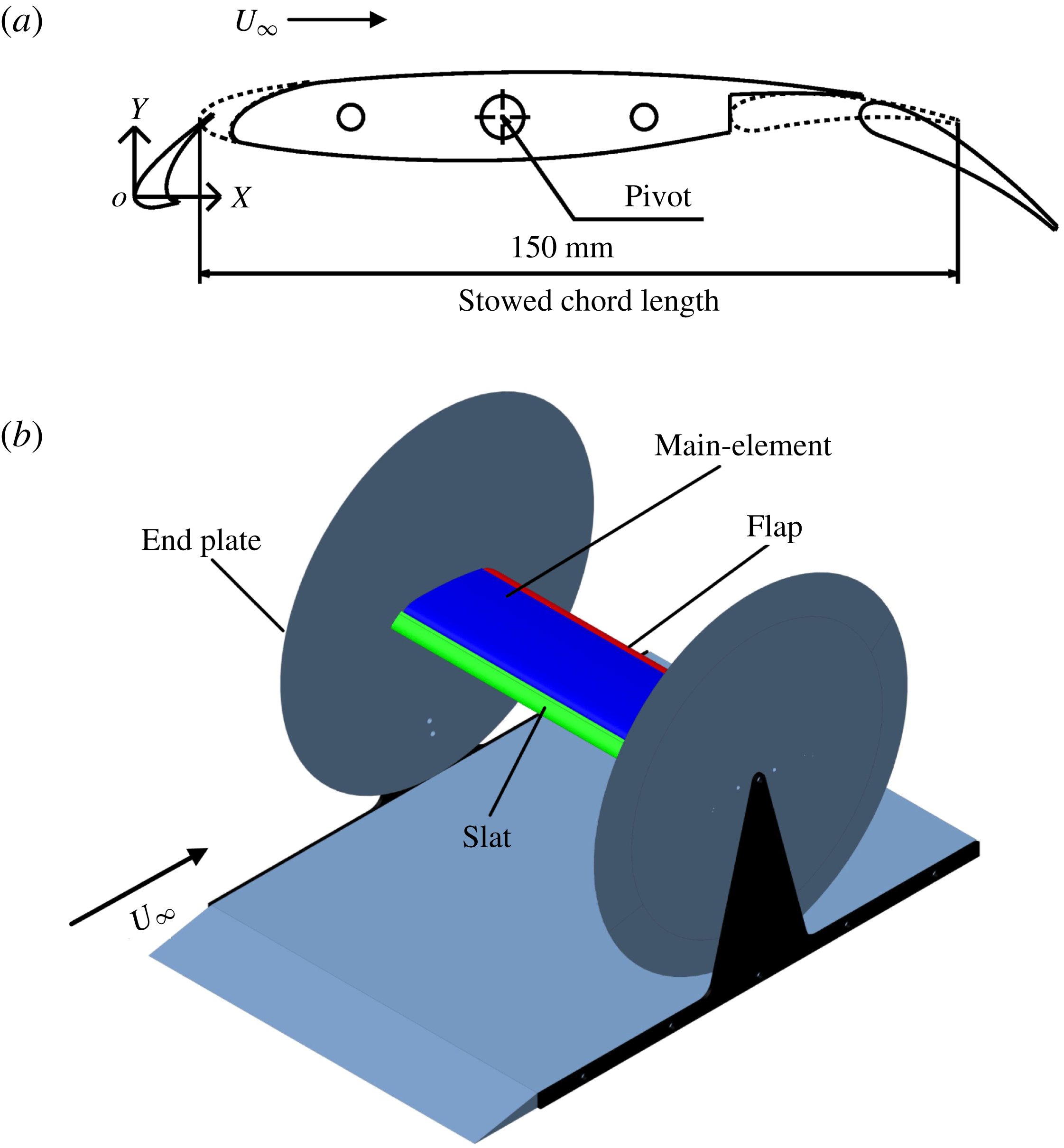
Reference Souza, Rodríguez, Simões and Medeiros2015). The 30P30N airfoil utilized in the current experiment is a scaled model from the AIAA BANC-II Workshop (Choudhari & Yamamoto Reference Choudhari and Yamamoto2012). As shown in figure 1(a), the stowed chord length
 $c$
is 150 mm. The aspect ratio is 3.33. According to Jenkins et al. (Reference Jenkins, Khorrami and Choudhari2004), this aspect ratio could ensure the quasi-two-dimensionality of the flow in the middle region of the airfoil. The angle of attack of the 30P30N airfoil (
 $\unicode[STIX]{x1D6FC}$
) is defined as the angle between the chord line of the main element and the horizontal line. Following this definition, the angle of attack in figure 1(a) is
 $\unicode[STIX]{x1D6FC}=0^{\circ }$
. Except for a few special definitions for local coordinate systems, the origin of the coordinate system (
 $O$
in figure 1
a) is located at the leading edge of the slat with
 $\unicode[STIX]{x1D6FC}=0^{\circ }$
.
 $X$
,
 $Y$
and
 $Z$
denote the streamwise, vertical and spanwise directions, respectively. As shown in figure 1(b), two circular acrylic endplates (radii equal to 250mm) with cut corners are applied at two sides of the airfoil. These two endplates could improve the mean spanwise uniformity of the airfoil flow (Boutilier & Yarusevych Reference Boutilier and Yarusevych2012a
).
 $\unicode[STIX]{x1D6FC}$
is adjusted by rotating the airfoil around the pivot.
(a) The 30P30N multi-element airfoil; (b) three-dimensional sketch for the installation of 30P30N airfoil.

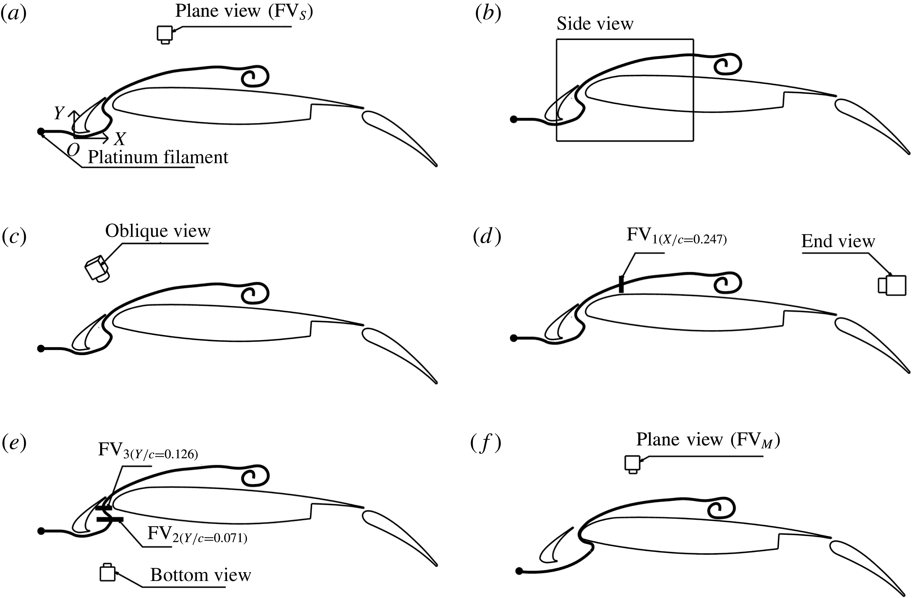
Sketch of hydrogen bubble flow visualization at
 $\unicode[STIX]{x1D6FC}=4^{\circ }$
: (a) plane view with volume illumination
 $(\text{FV}_{S})$
; (b) side view with a vertical laser sheet; (c) oblique view with volume illumination; (d) end view with a transverse laser sheet
 $(\text{FV}_{1})$
; (e) bottom view with two parallel horizontal laser sheets (
 $\text{FV}_{2}$
and
 $\text{FV}_{3}$
); (f) plane view with volume illumination
 $(\text{FV}_{M})$
.

2.2 Experimental set-up
The experiments are conducted in a water tunnel of the Institute of Fluid Mechanics at the Beijing University of Aeronautics and Astronautics. The test section is
 $600\times 600\times 3000~\text{mm}$
(height
 $\times$
width
 $\times$
length). The free-stream velocity is
 $U_{\infty }=60~\text{mm}~\text{s}^{-1}$
, with turbulence intensity less than 1 %. The Reynolds number based on the stowed chord length is
 $Re_{c}=8320$
. The flows over the multi-element airfoil with
 $\unicode[STIX]{x1D6FC}=0{-}16^{\circ }$
(the angle interval is
 $2^{\circ }$
) are investigated. To keep the description briefly, only the experimental set-up at
 $\unicode[STIX]{x1D6FC}=4^{\circ }$
is introduced in this section.
2.2.1 Hydrogen bubble flow visualization
Experimental set-up for hydrogen bubble flow visualization is illustrated in figure 2. A horizontal platinum filament is placed upstream of the slat to generate hydrogen bubble curtain. The hydrogen bubble curtain strikes the forward stagnation point of the slat and passes through the gap region between the slat and the main element. In figure 2(a), a digital video camera (DV) combined with volume illumination is applied to the plane view measurement (
 $\text{FV}_{S}$
). In figure 2(b), a CMOS camera combined with a vertical laser sheet is utilized for the side view measurement. Due to the complex geometry around the gap region, two semiconductor continuous lasers (8-W, 532 nm) are co-operated to illuminate the gap region. A slice of the hydrogen bubble curtain, illuminated by the laser sheet, is recorded as a streaky line. In order to emphasize the three-dimensional flow structures at
 $\unicode[STIX]{x1D6FC}=4^{\circ }$
, a DV in an oblique view is combined with the volume illumination to conduct the oblique view measurement (figure 2
c). A CMOS camera combined with a transverse laser sheet (
 $\text{FV}_{1}$
at
 $X/c=0.247$
) is applied to the end view measurement (figure 2
d). In figure 2(e), a DV combined with two parallel horizontal laser sheets (
 $\text{FV}_{2}$
at
 $Y/c=0.071$
and
 $\text{FV}_{3}$
at
 $Y/c=0.126$
) is utilized for the bottom view measurements. To visualize the flow structures around the main element, another plane view measurement (
 $\text{FV}_{M}$
) is conducted, as shown in figure 2(f). In this case, the horizontal platinum filament is downward shifted to make the hydrogen bubble curtain strike the forward stagnation point of the main element. The hydrogen bubble curtain passes through the gap region very close to the leading edge of the main element. The sampling frequencies of the DV and CMOS camera are 25 Hz and 50 Hz, respectively.
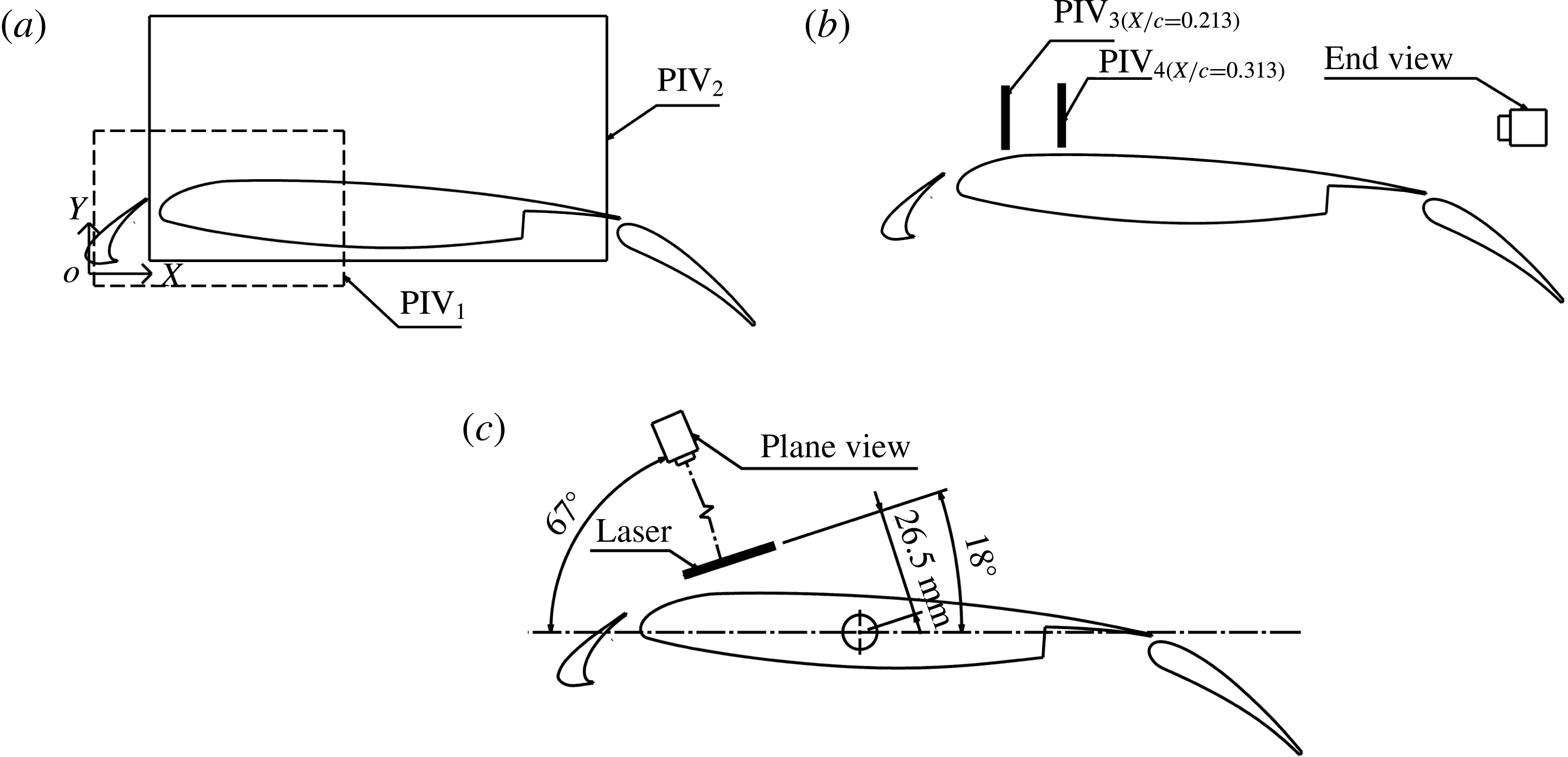
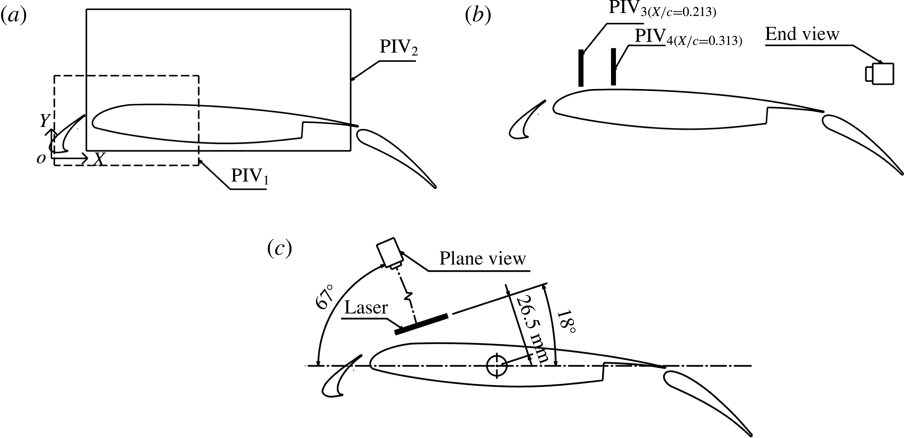
Experimental set-up for particle image velocimetry at
 $\unicode[STIX]{x1D6FC}=4^{\circ }$
: (a) side view with vertical laser sheets; (b) end view with transverse laser sheets; (c) plane view with an inclined laser sheet.
2.2.2 Particle image velocimetry
The two-dimensional time-resolved particle image velocimetry (TR-PIV) measurements are conducted to provide the quantitative information of the flow. Hollow glass beads with a typical diameter of
 $20~\unicode[STIX]{x03BC}\text{m}$
are utilized as tracer particles. To guarantee a high spatial resolution, two configurations, one focused on the gap flow and another focused on the flow around the main element, are utilized for the side view PIV measurements (
 $\text{PIV}_{1}$
and
 $\text{PIV}_{2}$
in figure 3
a). Two semiconductor continuous lasers (8-W, 532 nm) are co-operated to illuminate the gap region in configuration
 $\text{PIV}_{1}$
. Only one laser is applied for configuration
 $\text{PIV}_{2}$
. The experimental set-up for the end view PIV measurements (figure 3
b) is similar to the end view FV measurement (figure 2
d). Two transverse laser sheets (
 $\text{PIV}_{3}$
at
 $X/c=0.213$
and
 $\text{PIV}_{4}$
at
 $X/c=0.313$
) are respectively utilized to finish the measurements. According to the three-dimensional flow structures at
 $\unicode[STIX]{x1D6FC}=4^{\circ }$
, a plane view PIV measurement is conducted in the current work (figure 3
c). The FV results are utilized to determine the position of the laser sheet in figure 3(c). The image distortion is negligible in this configuration.
The sampling frequencies of the two side view PIV measurements are 120 Hz (
 $\text{PIV}_{2}$
with a magnification of
 $0.060~\text{mm}~\text{pix}^{-1}$
) and 180 Hz (
 $\text{PIV}_{1}$
with a magnification of
 $0.034~\text{mm}~\text{pix}^{-1}$
). Both the sampling frequencies of the two end view PIV measurements are at 50 Hz (
 $\text{PIV}_{3}$
with the magnification of
 $0.041~\text{mm}~\text{pix}^{-1}$
and
 $\text{PIV}_{4}$
with the magnification of
 $0.040~\text{mm}~\text{pix}^{-1}$
). The sampling frequency of the plane view PIV measurement is 200 Hz (with a magnification of
 $0.060~\text{mm}~\text{pix}^{-1}$
). The frequencies of the dominant flow structures in the current investigation are less than 3 Hz, one order of magnitude lower than all the sampling frequencies of the PIV measurements. Thus, these PIV measurements can be treated as time resolved. Most of the particles have diameters of around
 $3{-}4$
pixels in the images. Therefore, the peak-locking effect, an important contribution to the PIV uncertainty, is negligible (Christensen Reference Christensen2004). The velocity fields are calculated from the particle images by the Lucas–Kanade algorithm (Champagnat et al.
Reference Champagnat, Plyer, Le Besnerais, Leclaire, Davoust and Le Sant2011; Pan et al.
Reference Pan, Xue, Xu, Wang and Wei2015). This algorithm is based on the sum of square difference (SSD) optimization and is suitable for graphic processing units (GPU) acceleration (Champagnat et al.
Reference Champagnat, Plyer, Le Besnerais, Leclaire, Davoust and Le Sant2011; Pan et al.
Reference Pan, Xue, Xu, Wang and Wei2015). Multi-grid iteration with window deformation, as in the traditional cross-correlation algorithm (Scarano & Riethmuller Reference Scarano and Riethmuller2000), is also implicitly contained in the Lucas–Kanade algorithm (Pan et al.
Reference Pan, Xue, Xu, Wang and Wei2015) to improve the quality of the velocity field. According to different PIV configurations, the interrogation window sizes in the final pass are set to
 $32\times 32{-}40\times 40$
pixels with overlaps from 75 to 80 %. Under the utilization of both sub-pixel interpolation and multi-grid iteration with window deformation, the uncertainty of the particle displacement is less than 0.1 pixel. Both the maximum particle displacements in the two side view PIV measurements are approximately 15 pixels. Thus, the relative uncertainties of the particle displacements in these two measurements are estimated to be around 0.7 %
 $(0.1/15\approx 0.7\,\%)$
. Accordingly, the relative uncertainties of the particle displacements in the two end view PIV measurements are estimated to be around 0.9 %, and the plane view measurement is around 1.3 %. Finally, the relative uncertainties of the velocity in all the PIV measurements are estimated to be less than 2 %. At least 7000 snapshots are utilized for the statistics.
2.3 Post-processing tools
In order to facilitate a deep comprehension of the flow around the multi-element airfoil, a few post-processing tools are applied to the velocity fields. This section provides a brief introduction to these tools.
2.3.1 Proper orthogonal decomposition
Proper orthogonal decomposition (POD) (Berkooz, Holmes & Lumley Reference Berkooz, Holmes and Lumley1993; Chatterjee Reference Chatterjee2000) can be utilized to extract the dominant flow patterns from complex flow fields. In the current work, the fluctuation velocity field
 $\boldsymbol{U}^{\prime }(\boldsymbol{x},t)$
is utilized to conduct POD:
 $$\begin{eqnarray}\boldsymbol{U}^{\prime }(\boldsymbol{x},t)\approx \mathop{\sum }_{k=1}^{K}a_{k}(t)\unicode[STIX]{x1D731}_{k}(\boldsymbol{x}),\end{eqnarray}$$
where
 $a_{k}(t)$
is the energy-containing time coefficient of the
 $k$
th POD mode,
 $\unicode[STIX]{x1D731}_{k}(\boldsymbol{x})$
is the normalized
 $k$
th POD mode and
 $K$
is the truncation rank. The POD is calculated by solving the eigenvalue problem:
 $$\begin{eqnarray}\boldsymbol{C}a_{k}^{\ast }=\unicode[STIX]{x1D706}_{k}a_{k}^{\ast },\end{eqnarray}$$
where
 $\boldsymbol{C}=(\boldsymbol{U}^{\prime })^{\text{T}}\boldsymbol{U}^{\prime }$
,
 $\unicode[STIX]{x1D706}_{k}$
is the eigenvalue of
 $\boldsymbol{C}$
(represents the turbulent kinetic energy of the
 $k$
th POD mode) and
 $a_{k}^{\ast }$
is the
 $k$
th eigenvector of
 $\boldsymbol{C}$
(that represents the normalized time coefficient). The
 $k$
th POD mode
 $\unicode[STIX]{x1D731}_{k}(\boldsymbol{x})$
is obtained by projecting the fluctuation velocity field onto the normalized time coefficient (Mandal, Venkatakrishnan & Dey Reference Mandal, Venkatakrishnan and Dey2010):
 $$\begin{eqnarray}\unicode[STIX]{x1D731}_{k}(\boldsymbol{x})=\frac{\boldsymbol{U}^{\prime }a_{k}^{\ast }}{\Vert \boldsymbol{U}^{\prime }a_{k}^{\ast }\Vert },\end{eqnarray}$$
where
 $\Vert \bullet \Vert$
denotes the 2-norm. The energy-containing time coefficient of the
 $k$
th POD mode is obtained by providing the energy information to the normalized time coefficient:
 $$\begin{eqnarray}a_{k}(t)=\sqrt{\unicode[STIX]{x1D706}_{k}}a_{k}^{\ast }.\end{eqnarray}$$
Different POD modes can be selected to obtain the reconstructed fluctuation velocity field by (2.1). Mean velocity field can be superimposed to provide a reconstructed velocity field.
2.3.2 Oseen vortex fitting
Oseen vortex fitting has been successfully utilized to extract vortex dynamic information from turbulent flow (Carlier & Stanislas Reference Carlier and Stanislas2005). The potential vortices are fitted by the Oseen vortex template with a Gaussian-like vorticity distribution. The vortex core position, the circulation and the vortex radius can be extracted from the fitting results. Carlier & Stanislas (Reference Carlier and Stanislas2005) defined an isotropic parameter to remove the effect of a pure shear layer on the fitting results. In the current work, the criterion of swirl strength
 $\unicode[STIX]{x1D706}_{ci}$
(Zhou et al.
Reference Zhou, Adrian, Balachandar and Kendall1999; Ganapathisubramani, Longmire & Marusic Reference Ganapathisubramani, Longmire and Marusic2003) is utilized to remove the pure shear motions from the vorticity field rather than the isotropic parameter.
 $\unicode[STIX]{x1D706}_{ci}$
is defined as the magnitude of the imaginary part of the complex eigenvalues of the velocity gradient tensor. The Oseen vortex template fits the high-concentration region of
 $\unicode[STIX]{x1D706}_{ci}$
by a nonlinear least squares fitting algorithm (Levenberg–Marquardt method). The algorithm is detailed by Wang et al. (Reference Wang, Pan, Choi, Gao and Lian2013).
2.3.3 Finite-time Lyapunov exponents
Finite-time Lyapunov exponents (FTLE) method has been successfully utilized to track Lagrangian coherent structures (LCSs) (Haller & Yuan Reference Haller and Yuan2000; Haller Reference Haller2001; Shadden, Dabiri & Marsden Reference Shadden, Dabiri and Marsden2006; Green, Rowley & Haller Reference Green, Rowley and Haller2007; Shadden, Astorino & Gerbeau Reference Shadden, Astorino and Gerbeau2010). Using
 $\unicode[STIX]{x1D719}_{t_{0}}^{t_{0}+t_{1}}:\boldsymbol{y}(t_{0})\rightarrow \boldsymbol{y}(t_{0}+t_{1})$
denotes the flow map of fluid particles taken from the initial position
 $\boldsymbol{y}(t_{0})$
at
 $t_{0}$
to the location
 $\boldsymbol{y}(t_{0}+t_{1})$
at
 $t_{0}+t_{1}$
. In the current work, the locations
 $\boldsymbol{y}(t)$
are calculated from the discrete PIV velocity data (He et al.
Reference He, Pan, Feng, Gao and Wang2016). The FTLE at
 $t_{0}$
can be calculated as follows (Haller Reference Haller2001):
 $$\begin{eqnarray}\unicode[STIX]{x1D70E}(\boldsymbol{y},t_{0},t_{1})=\frac{1}{|2t_{1}|}\ln \left(\unicode[STIX]{x1D706}_{max}\left\{\left[\frac{\unicode[STIX]{x2202}\boldsymbol{y}(t_{0}+t_{1})}{\unicode[STIX]{x2202}\boldsymbol{y}(t_{0})}\right]^{\text{T}}\left[\frac{\unicode[STIX]{x2202}\boldsymbol{y}(t_{0}+t_{1})}{\unicode[STIX]{x2202}\boldsymbol{y}(t_{0})}\right]\right\}\right),\end{eqnarray}$$
where
 $\unicode[STIX]{x1D70E}(\boldsymbol{y},t_{0},t_{1})$
denotes the exponential growth rate of nearby trajectories over a finite time interval
 $t_{1}$
,
 $\unicode[STIX]{x1D706}_{max}$
represents the largest singular value of the deformation gradient matrix. LCSs are defined as the ridges of
 $\unicode[STIX]{x1D70E}(\boldsymbol{y},t_{0},t_{1})$
. Both
 $t_{1}>0$
and
 $t_{1}<0$
can be used to conduct forward and backward computations, respectively. However, only backward computations (
 $t_{1}<0$
) are utilized to obtain ridges with attracting properties in the current work.
Shadden, Lekien & Marsden (Reference Shadden, Lekien and Marsden2005) proved that the flux of particles through the ridge of FTLE was indeed negligible. Therefore, ridges within FTLE fields could be treated as virtual boundaries. This characteristic of the FTLE ridge is quite crucial in the current work.
2.3.4 Fourier mode decomposition
Fourier mode decomposition (FMD) can provide global frequency information of the whole flow field rather than the local frequency information of the single-point fast Fourier transformation (FFT) (Ma et al.
Reference Ma, Feng, Pan, Gao and Wang2015). For the chosen flow region, single-point discrete Fourier transformation (DFT) is applied to velocity data at every mesh point to obtain a Fourier transform matrix
 $\unicode[STIX]{x1D658}_{k}$
:
 $$\begin{eqnarray}\unicode[STIX]{x1D658}_{k}=\frac{1}{N}\mathop{\sum }_{n=0}^{N-1}\unicode[STIX]{x1D641}_{n}\text{e}^{-\text{i}(2\unicode[STIX]{x03C0}k/N)n},\end{eqnarray}$$
where
 $N$
is the total sampling number, and
 $\unicode[STIX]{x1D641}_{n}$
is the original velocity matrix. The global power spectrum density (
 $\text{PSD}_{k}$
) is defined as follows:
 $$\begin{eqnarray}\text{PSD}_{k}=\left\Vert \frac{2N|\unicode[STIX]{x1D658}_{k}|^{2}}{\unicode[STIX]{x03C0}\boldsymbol{f}_{\boldsymbol{s}}}\right\Vert ,\end{eqnarray}$$
where
 $\Vert \bullet \Vert$
is the Frobenius norm of all single-point power spectrum densities,
 $\boldsymbol{f}_{\boldsymbol{s}}$
is the sampling frequency.
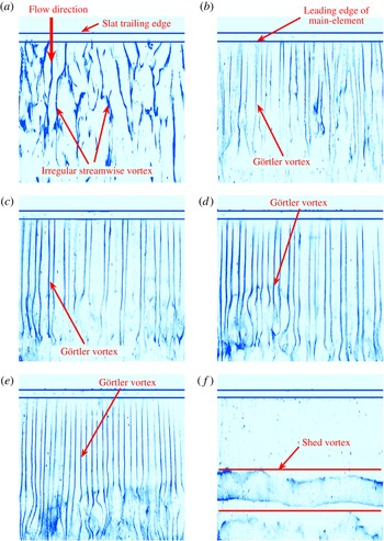
Plane view flow visualization with volume illumination (
 $\text{FV}_{S}$
): (a)
 $\unicode[STIX]{x1D6FC}=0^{\circ }$
; (b)
 $\unicode[STIX]{x1D6FC}=2^{\circ }$
; (c)
 $\unicode[STIX]{x1D6FC}=4^{\circ }$
; (d)
 $\unicode[STIX]{x1D6FC}=8^{\circ }$
; (e)
 $\unicode[STIX]{x1D6FC}=12^{\circ }$
; (f)
 $\unicode[STIX]{x1D6FC}=16^{\circ }$
. The horizontal platinum filament in figure 2(a) is shifted to the slat trailing edge to improve the quality of these images. The high-concentration regions of hydrogen bubbles (blue colour in these images) represent the vortices.

Vorticity contours of the side view PIV results at
 $\unicode[STIX]{x1D6FC}=0^{\circ }$
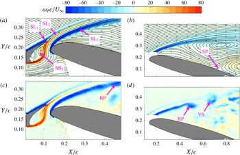
: (a) average vorticity contour of the gap flow; (b) average vorticity contour of the flow around the main element; (c) instantaneous vorticity contour of the gap flow; (d) instantaneous vorticity contour of the flow around the main element. The streamlines of the mean flow are superimposed in (a) and (b).

3 Results and discussion
3.1 Dominant flow structures
According to the evolution of dominant flow structures around the main element with angles of attack (
 $\unicode[STIX]{x1D6FC}=0^{\circ }{-}16^{\circ }$
with an interval
 $2^{\circ }$
), three regimes can be classified in the current work, as shown in figure 4: (i) irregular streamwise vortex at
 $\unicode[STIX]{x1D6FC}=0^{\circ }$
(figure 4
a); (ii) regular streamwise vortex, named the Görtler vortices, at
 $\unicode[STIX]{x1D6FC}=2{-}12^{\circ }$
(figure 4
b–e); (iii) two-dimensional spanwise shed vortex at
 $\unicode[STIX]{x1D6FC}=14^{\circ }{-}16^{\circ }$
(figure 4
f). It should be emphasized that the Görtler vortices are first observed in the flow around multi-element airfoil and are the focus of the current work. In this section,
 $\unicode[STIX]{x1D6FC}=0$
,
 $\unicode[STIX]{x1D6FC}=4^{\circ }$
and
 $\unicode[STIX]{x1D6FC}=16^{\circ }$
are respectively taken as the representative cases of the three regimes to be further explored. The quantities associated with length are normalized by the stowed chord length
 $c$
, and those associated with velocity are normalized by the free-stream velocity
 $U_{\infty }$
.
3.1.1
 $\unicode[STIX]{x1D6FC}=0^{\circ }$

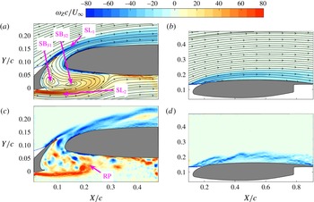
Figure 5 presents the vorticity contours of the side view PIV results at
 $\unicode[STIX]{x1D6FC}=0^{\circ }$
. Four time-averaged structures dominate the gap flow (
 $\text{SL}_{1}$
,
 $\text{SL}_{2}$
,
 $\text{SB}_{S1}$
, and
 $\text{SB}_{\text{S2}}$
in figure 5
a). The separated shear layer
 $\text{SL}_{2}$
originates from the lower surface of the slat. This separated shear layer extends to the front stagnation point of the main element and could be bended by the main flow toward the leading edge of the main element. However, this shear layer cannot pass through the gap region. As indicated by the curving streamlines, two separation bubbles exist around the slat cove (
 $\text{SB}_{\text{S1 }}$
and
 $\text{SB}_{\text{S2}}$
in figure 5
a). The shear layer (
 $\text{SL}_{\text{1 }}$
in figure 5
a) originating from the upper surface of the slat could interact with the upper boundary layer of the main element to form a confluent boundary layer on the main element (figure 5
b). The parallel streamlines in figure 5(b) reveal that there is no time-averaged flow separation existing above the main element. However, the instantaneous vorticity contours (figure 5
c,d) indicate that there are separated shear layers existing above the main element. The roll up (RP) in figure 5(c) indicates that
 $\text{SL}_{2}$
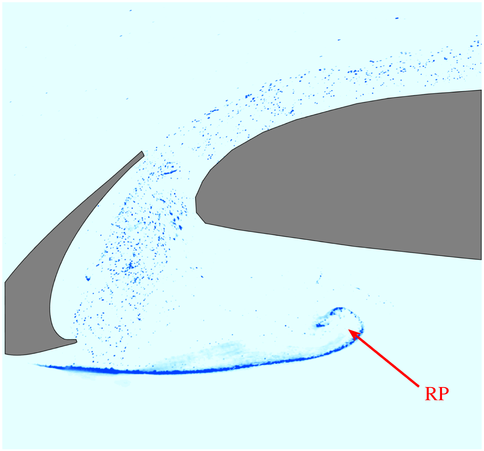
undergoes K–H instability. This roll up can also be captured by the FV result in figure 6. The roll up of
 $\text{SL}_{2}$
finally results in vortex shedding. The chaotic flow within the slat cove (figure 5
c) could be attributed to the breakdown of the shed vortex. This chaotic flow is consistent with the FV result (figure 6) that the hydrogen bubble curtain loses the concentrated property rapidly after the roll up of
 $\text{SL}_{2}$
. As indicated in previous numerical simulations (Deck & Laraufie Reference Deck and Laraufie2013; Meyer et al.
Reference Meyer, Hickel, Breitsamter and Adams2013; Choudhari & Lockard Reference Choudhari and Lockard2015; Lockard et al.
Reference Lockard, Choudhari and Buning2015; Terracol et al.
Reference Terracol, Manoha, Murayama, Yamamoto, Amemiya and Tanaka2015), the spanwise vortices within the chaotic flow of the slat cove could be deformed into streamwise vortices by the accelerated gap flow. This mechanism could contribute to the formation of the irregular streamwise vortex above the main element (figure 4
a).
Side view flow visualization at
 $\unicode[STIX]{x1D6FC}=0^{\circ }$
.

3.1.2
$\unicode[STIX]{x1D6FC}=4^{\circ }$

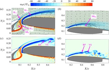
In figure 7(a), the shear layer (
 $\text{SL}_{1}$
) originating from the upper surface of the slat may merge with the shear layer (
 $\text{SL}_{3}$
) originating from the leading-edge separation of the main element. A meandering shear layer (
 $\text{SL}_{2}$
) originating from the lower surface of the slat exists in the gap region. As the backward-facing step (Barkley, Gomes & Henderson Reference Barkley, Gomes and Henderson2002; Beaudoin et al.
Reference Beaudoin, Cadot, Aider and Wesfreid2004) or cavity flow (Faure et al.
Reference Faure, Adrianos, Lusseyran and Pastur2007, Reference Faure, Pastur, Lusseyran, Fraigneau and Bisch2009; Faure Reference Faure2014; Douay, Pastur & Lusseyran Reference Douay, Pastur and Lusseyran2016a
), a separation bubble (
 $\text{SB}_{S}$
) exists in the slat cove. Both
 $\text{SB}_{S}$
and the leading edge of the main element contribute to the meandering main flow within the gap region. In figure 7(b), another separation bubble (
 $\text{SB}_{M}$
) on the main element is revealed by the streamlines. According to the instantaneous vorticity contours, both figures 7(c) and 7(d) capture the roll up of
 $\text{SL}_{3}$
(RP) and the following shed vortex (VS), which are the results of K–H instability. The shed vortex may facilitate the reattachment of
 $\text{SL}_{3}$
to form
 $\text{SB}_{M}$
in figure 7(b) (Hain et al.
Reference Hain, Kähler and Radespiel2009; Mcauliffe & Yaras Reference Mcauliffe and Yaras2009; Simoni et al.
Reference Simoni, Ubaldi, Zunino, Lengani and Bertini2012; Marxen et al.
Reference Marxen, Lang and Rist2013; Lengani et al.
Reference Lengani, Simoni, Ubaldi and Zunino2014; Kurelek et al.
Reference Kurelek, Lambert and Yarusevych2016). The chaotic structures after
 $X/c=0.667$
above the main element indicate that the flow around this region is not in a laminar state any more. No shed vortex emanating from the K–H instability of
 $\text{SL}_{2}$
exists within the gap flow (figure 7
c). Therefore, the formation of
 $\text{SB}_{S}$
is attributed to a laminar reattachment (Beaudoin et al.
Reference Beaudoin, Cadot, Aider and Wesfreid2004) rather than a turbulent reattachment. This is quite different from the PIV results of Jenkins et al. (Reference Jenkins, Khorrami and Choudhari2004) (
 $Re_{c}=3.64\times 10^{6}$
,
 $\unicode[STIX]{x1D6FC}=4^{\circ }$
). This disparity could be attributed to the low Reynolds number in the current investigation. There is also no vortex shedding at the trailing edge of the slat, which is different from both the vortex shedding emanating from the blunt slat trailing edge (Jenkins et al.
Reference Jenkins, Khorrami and Choudhari2004) and that emanating from the global instability of the laminar slat wake (Makiya et al.
Reference Makiya, Inasawa and Asai2010). Differences between Jenkins et al. (Reference Jenkins, Khorrami and Choudhari2004) and the current investigation could still be attributed to different Reynolds numbers. However, except for the difference of the Reynolds number, the disparity on the slat angle could also contribute to the different flow structures between Makiya et al. (Reference Makiya, Inasawa and Asai2010) and the current investigation.
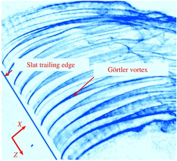
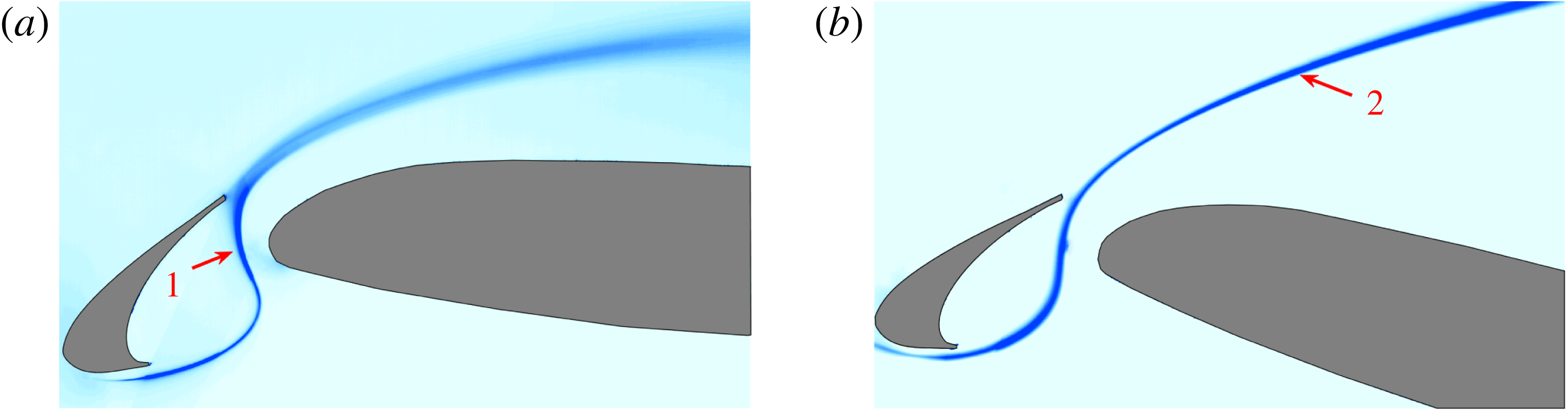
Figure 8 provides a three-dimensional view of Görtler vortices. It can be seen that these vortices originate from the gap region and are dominant structures before the occurrence of the shed vortex (VS in figure 7). Thus, these longitudinal vortices cannot be the longitudinal braid vortices, which exist after the occurrence of a shed vortex (Jones et al. Reference Jones, Sandberg and Sandham2008; Marxen et al. Reference Marxen, Lang and Rist2013; Kurelek et al. Reference Kurelek, Lambert and Yarusevych2016). As Görtler vortices generally occur in the concave boundary layer, the existence of this kind of flow structure above the convex suction surface of the main element is quite amazing. The characteristics and the origin of the Görtler vortices will be focused on below.
Vorticity contours of the side view PIV results at
 $\unicode[STIX]{x1D6FC}=4^{\circ }$
: (a) average vorticity contour of the gap flow; (b) average vorticity contour of the flow around the main element; (c) instantaneous vorticity contour of the gap flow; (d) instantaneous vorticity contour of the flow around the main element. The streamlines of the mean flow are superimposed in (a) and (b).

Oblique view flow visualization at
 $\unicode[STIX]{x1D6FC}=4^{\circ }$
. Both the streamwise direction and the spanwise direction are marked in this figure.

Vorticity contours of the side view PIV results at
 $\unicode[STIX]{x1D6FC}=16^{\circ }$
: (a) average vorticity contour of the gap flow; (b) average vorticity contour of the flow around the main element; (c) instantaneous vorticity contour of the gap flow; (d) instantaneous vorticity contour of the flow around the main element. The streamlines of the mean flow are superimposed in (a) and (b).

Side view flow visualization at
 $\unicode[STIX]{x1D6FC}=16^{\circ }$
.

3.1.3
$\unicode[STIX]{x1D6FC}=16^{\circ }$

Several time-averaged dominant flow structures (
 $\text{SL}_{1}$
,
 $\text{SL}_{2}$
,
 $\text{SL}_{3}$
and
 $\text{SB}_{S}$
) at
 $\unicode[STIX]{x1D6FC}=4^{\circ }$
can still be captured at
 $\unicode[STIX]{x1D6FC}=16^{\circ }$
(figure 9
a). The nomenclatures in figure 7(a) are still utilized in figure 9(a). Compared with that at
 $\unicode[STIX]{x1D6FC}=4^{\circ }$
, the size of
 $\text{SB}_{S}$
is smaller at
 $\unicode[STIX]{x1D6FC}=16^{\circ }$
. The smaller
 $\text{SB}_{S}$
results in a less meandering main flow within the gap region than that at
 $\unicode[STIX]{x1D6FC}=4^{\circ }$
. Shed vortex emanating from
 $\text{SL}_{3}$
(VS in figure 9
d) still exists at
 $\unicode[STIX]{x1D6FC}=16^{\circ }$
. However, the shed vortex cannot result in the reattachment of
 $\text{SL}_{3}$
(figure 9
b). Therefore, no separation bubble is formed above the main element. A stagnation point (SP in figure 9
b) exists on the upper surface of the main element. Except for VS, no other shed vortex can be captured from figure 9(c,d). It should be emphasized that there is no Görtler vortices existing at
 $\unicode[STIX]{x1D6FC}=16^{\circ }$
(figure 4
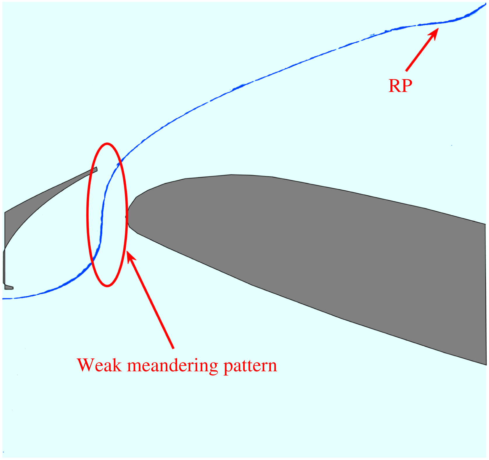
f). The hydrogen bubble curtain will pass through the gap region in a weak meandering way (figure 10). The meandering path is consistent with the results shown in figure 9. As indicated in figure 4(f), the hydrogen bubble curtain has good two-dimensionality and is rolled up (RP in figure 10) to form the two-dimensional spanwise vortex as shown in figure 4(f).
3.2 Travelling motion of the Görtler vortices
In this section, the characteristics of the Görtler vortices at
 $\unicode[STIX]{x1D6FC}=4^{\circ }$
are discussed in detail. Travelling motion of the Görtler vortices in the spanwise direction and secondary vortices underneath the Görtler vortices are presented. The spanwise wavelength of the Görtler vortices is also provided in this part.
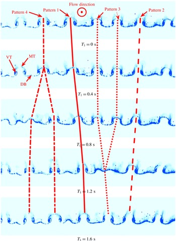
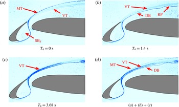
In figure 11, the classical mushroom-shaped patterns are captured, which are typical topological structures of Görtler vortices (Floryan Reference Floryan1991) or Dean vortices (Ligrani & Niver Reference Ligrani and Niver1988). These patterns are also indicators of the nonlinear evolution of Görtler vortices (Winoto & Shah Reference Winoto and Shah2008). The upwash and downwash motions induced by the counter-rotating vortices make the horizontal hydrogen bubble curtain warp (MT and DB in figure 11). Four time-evolved patterns of Görtler vortices are marked in figure 11. Pattern 1 and pattern 2 show that the Görtler vortices travel right and left along the spanwise direction respectively. It is revealed in pattern 3 that two pairs of counter-rotating vortices could be replaced by one pair of counter-rotating vortices. Meanwhile, one pair of counter-rotating vortices could be replaced by two pairs of counter-rotating vortices, as shown in pattern 4. Pattern 4 has been reported on the Dean vortices over a concave wall (Ligrani & Niver Reference Ligrani and Niver1988).
End view FV results (
 $\text{FV}_{1}$
,
 $X/c=0.247$
). The trace lines display different flow patterns. The bottom of each image is located on the surface of the main element. The top of the mushroom-shaped pattern is marked MT. The streaky line between two mushroom-shaped patterns is marked DB. The vortex tube of the counter-rotating vortices is marked VT. The main flow direction points outside of the measurement plane.

(a) Oseen vortex fitting of an instantaneous end view PIV snapshot at
 $X/c=0.313\,(\text{PIV}_{4})$
; (b) space–time diagram of
 $\unicode[STIX]{x1D706}_{ci}$
built from the sample position at (a); (c) space–time diagram of
 $\unicode[STIX]{x1D706}_{ci}$
built from the sample position at (a). The
 $\unicode[STIX]{x1D706}_{ci}$
contour with the sign of the vorticity is shown as the background in (a). The fitting vortex cores are marked by
 $\times$
in (a). The fitting vortices are denoted by black circles in (a). The origin of the local coordinate system is located at the bottom left corner of the field of view. The local vertical direction and the local spanwise direction are denoted
 $Y_{L2}$
and
 $Z_{L2}$
respectively. The line
 $Y_{L2}/c=0$
denotes the surface of the main element. Similarly, subscript
 $L1$
is utilized for the local coordinate system of the end view PIV measurement at
 $X/c=0.213$
(
 $\text{PIV}_{3}$
). The main flow direction points outside of the measurement plane.

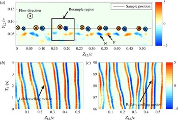
In figure 12(a), the instantaneous
 $\unicode[STIX]{x1D706}_{ci}$
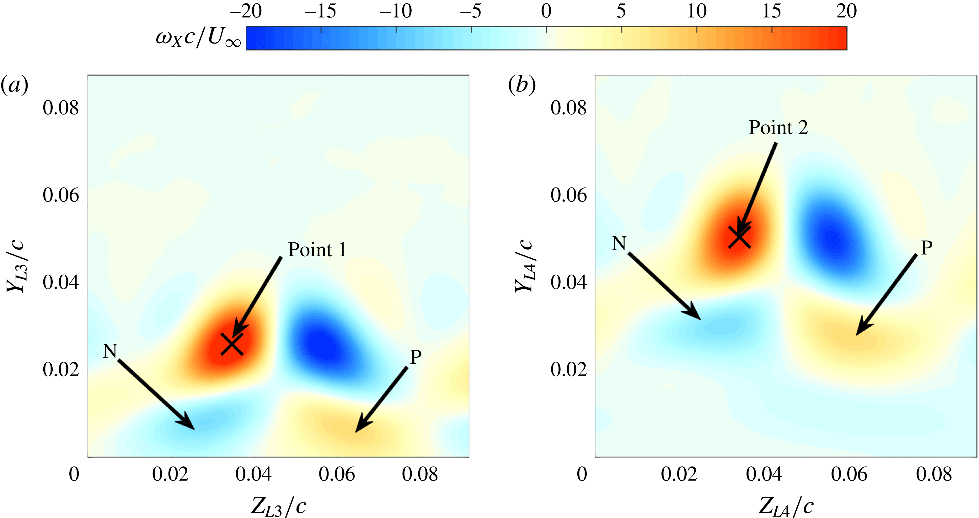
contour is shown with the results of Oseen vortex fitting. The counter-rotating vortices are clearly captured by this fitting method. The spanwise wavelength of the Görtler vortices is not identical. This non-uniform phenomenon is quite normal for naturally developed (no pre-set disturbance) Görtler vortices (Swearingen & Blackwelder Reference Swearingen and Blackwelder1987; Finnis & Brown Reference Finnis and Brown1997) and could be attributed to the non-uniform initial disturbances (Winoto, Mitsudharmadi & Shah Reference Winoto, Mitsudharmadi and Shah2005). Pattern 2 and pattern 1 can also be captured in figure 12(b,c). The unsteady travelling motion of the Görtler vortices is quite different from the classical stationary Görtler vortices (Floryan Reference Floryan1991; Saric Reference Saric1994). The interpretation of this unsteady phenomenon will be provided in § 3.5. It can be seen that the secondary counter-rotating vortices (N and P in figure 12
a) emerge beneath the main Görtler vortices. These secondary vortices have opposite rotation compared with the main Görtler vortices. In order to verify the relationship between the main Görtler vortices and the secondary vortices, the conditional average results are shown in figure 13. According to the position of the left vortex core (with positive vorticity), a resample region associated with one pair of counter-rotating vortices is defined in figure 12(a). The velocity data within all the resample regions are extracted to conduct the conditional average by aligning the positions of the vortex cores (point 2 in figure 13
b). Accordingly, the conditional average of the end view PIV result at
 $X/c=0.213$
is conducted in the similar way (figure 13
a). Ultimately, the secondary vortices with opposite rotation direction to the main Görtler vortices are clearly captured in the vorticity contours of the conditional average results (N and P in figure 13). The influences of these secondary vortices on
 $\text{SL}_{3}$
will be discussed in § 3.4. It should be emphasized that the term Görtler vortices is utilized to refer to the primary vortex.
Vorticity contours of the conditional average of the end view PIV results: (a) plane at
 $X/c=0.213$
; (b) plane at
 $X/c=0.313$
. In (b), the origin of the local coordinate system is located at the bottom left corner of the resampling region in figure 12(a). The local vertical direction and the local spanwise direction are denoted as
 $Y_{L4}$
and
 $Z_{L4}$
respectively. Similarly, subscript
 $L3$
is utilized for the local coordinate system of the plane at
 $X/c=0.213$
.

(a) Contour of two-point correlation
 $R$
at
 $X/c=0.313$
; (b) profile of the correlation coefficient at the sample position in (a). The local peaks in (a) and (b) are marked as black
 $\times$
.

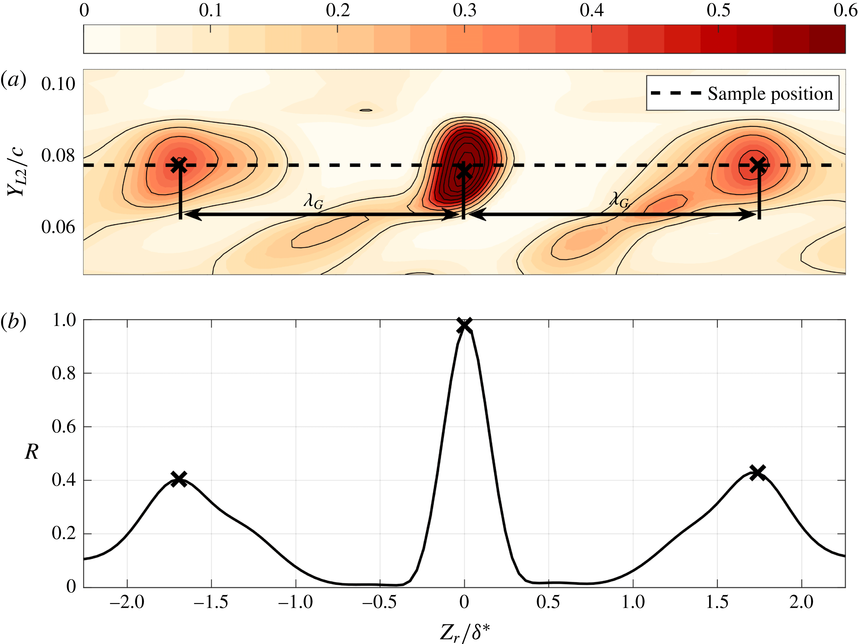
Two-point correlation is utilized to provide the spanwise wavelength information of the Görtler vortices at
 $X/c=0.313$
. This method has been utilized to conduct the correlation between velocity and
 $\unicode[STIX]{x1D706}_{ci}$
to capture the inclined hairpin packets in turbulent flow (Christensen & Adrian Reference Christensen and Adrian2001). However, this method is used to conduct correlation between
 $\unicode[STIX]{x1D706}_{ci}$
with positive sign (
 $\unicode[STIX]{x1D6EC}_{ci}$
) in the current work. The details are as follows:
 $$\begin{eqnarray}R(Z_{r},Y_{L2})=\frac{\langle \unicode[STIX]{x1D6EC}_{ci}(Z_{L2},y_{ref})\unicode[STIX]{x1D6EC}_{ci}(Z_{L2}+Z_{r},Y_{L2})\rangle }{\langle \unicode[STIX]{x1D6EC}_{ci}(Z_{L2},y_{ref})\unicode[STIX]{x1D6EC}_{ci}(Z_{L2},y_{ref})\rangle },\end{eqnarray}$$
where
 $Z_{L2}$
and
 $Y_{L2}$
follow the definition in figure 12,
 $y_{ref}$
denotes the reference position of the correlation (
 $Y_{L2}/c=0.0728$
) and
 $\langle \bullet \rangle$
denotes the inner product. Finally, the two-point correlation coefficient
 $R$
is shown in figure 14. To display the results clearly, only a portion of
 $R$
is provided in figure 14(a) with a zoomed-in view. The spanwise periodic property of the Görtler vortices is captured by these correlation coefficients distinctly. Since the spanwise wavelength of the Görtler vortices is non-uniform, the wavelength extracted from the distance between the local peaks of the correlation coefficients (
 $\unicode[STIX]{x1D706}_{G}$
in figure 14) could represent the most likely dominant wavelength. The local boundary layer displacement thickness
 $\unicode[STIX]{x1D6FF}^{\ast }$
at
 $X/c=0.313$
is applied to normalize the wavelength (Matsubara & Alfredsson Reference Matsubara and Alfredsson2001; Schlatter et al.
Reference Schlatter, Brandt, De Lange and Henningson2008):
 $$\begin{eqnarray}\unicode[STIX]{x1D6FF}^{\ast }=\int _{0}^{\unicode[STIX]{x1D6FF}}(1-U(Y_{L2})/U_{\unicode[STIX]{x1D6FF}})\,\text{d}Y_{L2},\end{eqnarray}$$
where
 $\unicode[STIX]{x1D6FF}$
denotes the position of the separatrix between the slat wake and the separation bubble above the main element,
 $U_{\unicode[STIX]{x1D6FF}}$
represents the streamwise velocity at
 $\unicode[STIX]{x1D6FF}$
. Ultimately, the non-dimensional wavelength of the Görtler vortices at
 $\unicode[STIX]{x1D6FC}=4^{\circ }$
is approximately 1.72. This value is smaller than the streak spacing in the transitional boundary layer (with adverse streamwise pressure gradient) induced by free-stream turbulence (FST), which is approximately located at the range of
 $6{-}8\unicode[STIX]{x1D6FF}^{\ast }$
(Brinkerhoff & Yaras Reference Brinkerhoff and Yaras2015; Lengani et al.
Reference Lengani, Simoni, Ubaldi, Zunino and Bertini2017). This difference in wavelength indicates that the generation mechanism of counter-rotating vortices in the current work is different from that of streaky structures in the FST-induced transitional boundary layer. The variation of the absolute value of the dominant wavelength is insensitive to the variation of angle of attack in the current measurement. The root-mean-square of the non-uniform wavelength is provided by Oseen vortex fitting. The distance between two left vortex cores (with positive vorticity) is defined as the wavelength between two pairs of Görtler vortices. The non-dimensional dominant wavelength calculated from Oseen vortex fitting is also around 1.72, which is nearly the same with the result of two-point correlation. The non-dimensional root-mean-square value of this dominant wavelength is approximately 0.31, which is 18 % of the dominant wavelength.
3.3 Footprints of the travelling Görtler vortices
In this section, the footprints of the travelling Görtler vortices are determined in the side view PIV measurements at
 $\unicode[STIX]{x1D6FC}=4^{\circ }$
. These footprints reveal that the Görtler vortices reside on the separated shear layer originating from the leading-edge separation of the main element (
 $\text{SL}_{3}$
in figure 7). The secondary counter-rotating vortices are found within the separated shear layer. Besides, the different statistical properties of several parameters between
 $\unicode[STIX]{x1D6FC}=4^{\circ }$
and
 $\unicode[STIX]{x1D6FC}=16^{\circ }$
, resulting from whether Görtler vortices exist in the flow or not, are also addressed in this part.
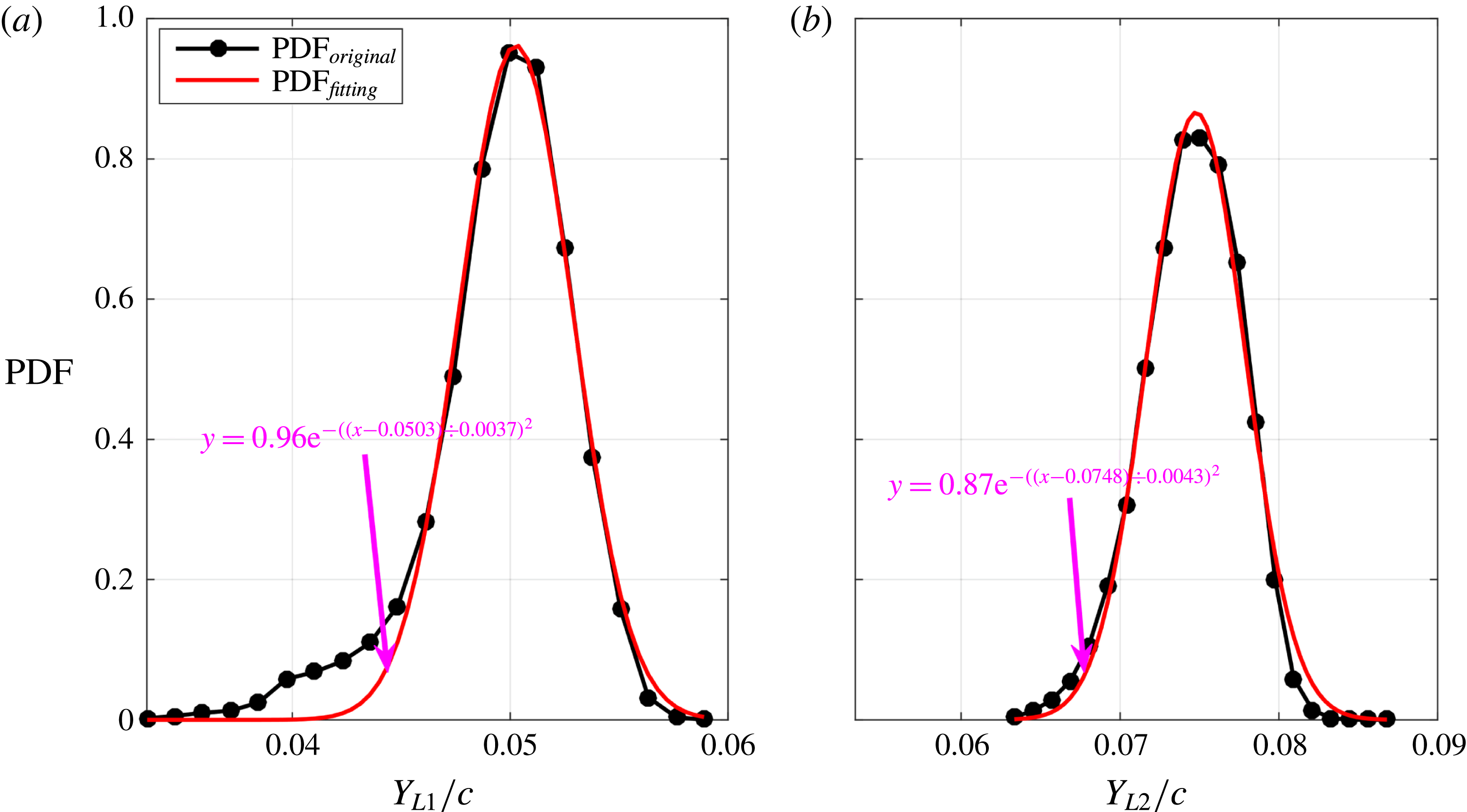
In figure 15, the probability density functions (PDF) of the vertical positions of the Görtler vortices cores are shown at two streamwise locations (
 $X/c=0.213$
and
 $X/c=0.313$
). The PDF calculated from the experimental data can be fitted well with a Gaussian function, except for the deviation at
 $Y_{L1}/c=0.04{-}0.043$
in figure 15(a). The peaks of Gaussian fittings are chosen as the dominant vertical positions at these two streamwise locations:
 $Y_{L1}/c=0.0503$
at
 $X/c=0.213$
and
 $Y_{L2}/c=0.0748$
at
 $X/c=0.313$
.
Probability density functions of the vertical positions of Görtler vortices cores: (a)
 $X/c=0.213$
; (b)
 $X/c=0.313$
. The original PDF is denoted by the black line with dark spots. The Gaussian fitting of the original PDF is denoted by the red line. The pink function provides the parameters of the Gaussian fitting.

(a) Mean velocity profiles at
 $X/c=0.213$
; (b) mean velocity profiles at
 $X/c=0.313$
; (c) root-mean-square of velocity fluctuations at
 $X/c=0.213$
; (d) root-mean-square of velocity fluctuations at
 $X/c=0.313$
. The black and red lines represent the profiles associated with streamwise and vertical velocities, respectively. The vertical positions of Görtler vortices cores are marked as blue pentagrams.

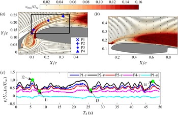
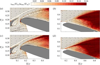
(a) Root-mean-square contour of the vertical fluctuation velocity from the PIV results focused on the gap flow; (b) root-mean-square contour of the vertical fluctuation velocity from the PIV results focused on the flow around the main element; (c) time sequences of velocity at different virtual probe positions in (a). The streamlines of the mean flow are superimposed in (a) and (b). All the virtual probes in (a) are located at the local peaks of
 $v_{rms}/U_{\infty }$
. The fluctuation velocity within the black box in (
 $a$
) is extracted for the POD in figure 20. Only the vertical components of the velocity are shown at P2, P3 and P4 in (c). Both the vertical and the streamwise components of the velocity are shown at P1 in (c). The instants I1, I2, I3 and I4 are chosen for the FTLE calculation in figure 19.

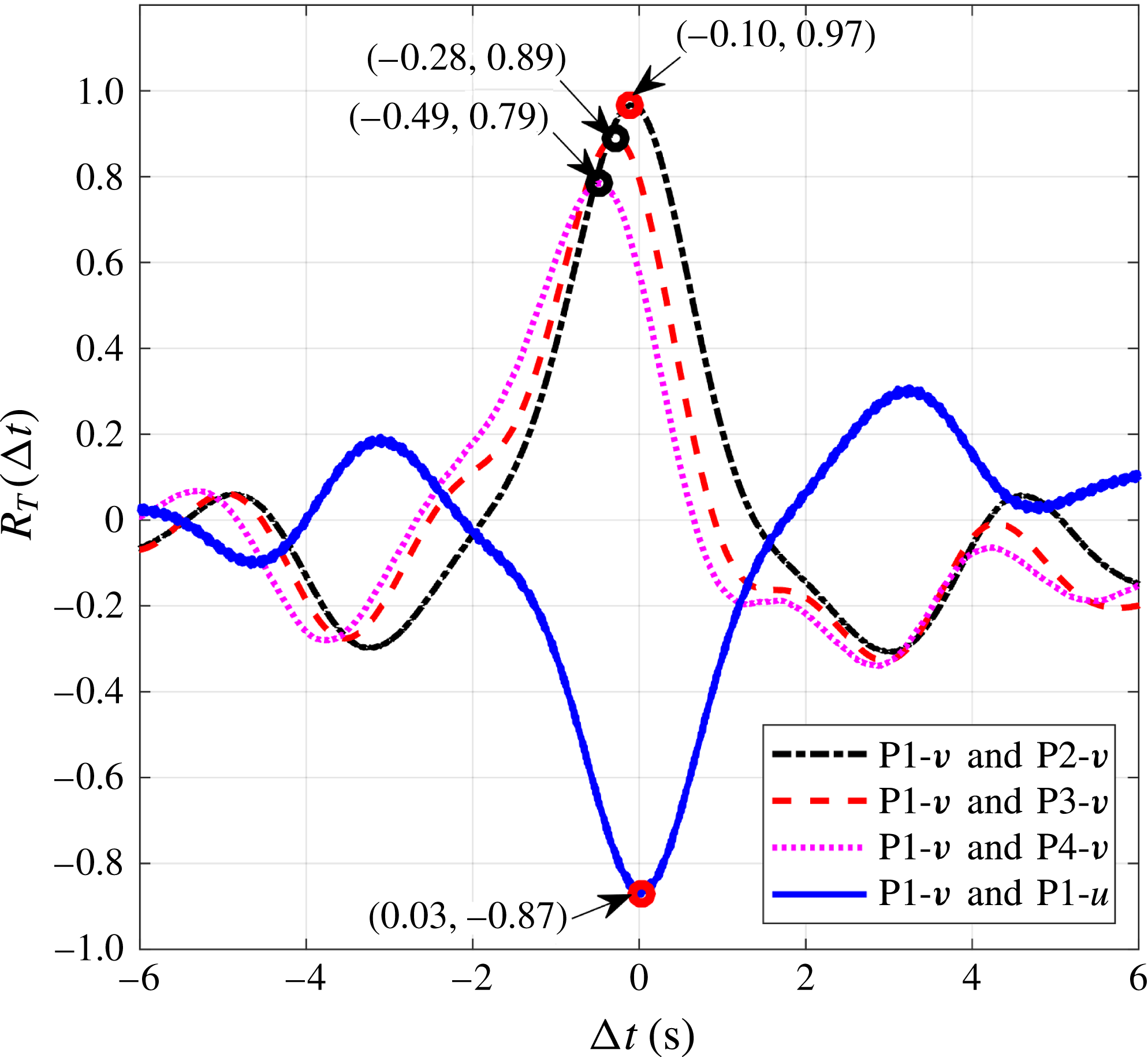
Time-shift correlation coefficients between different velocity sequences. Only the correlation coefficients with
 $-6<\unicode[STIX]{x0394}t<6$
are provided in this figure to ensure clarity. Both the time shifts and the correlation coefficients related to the maxima are denoted by arrows.


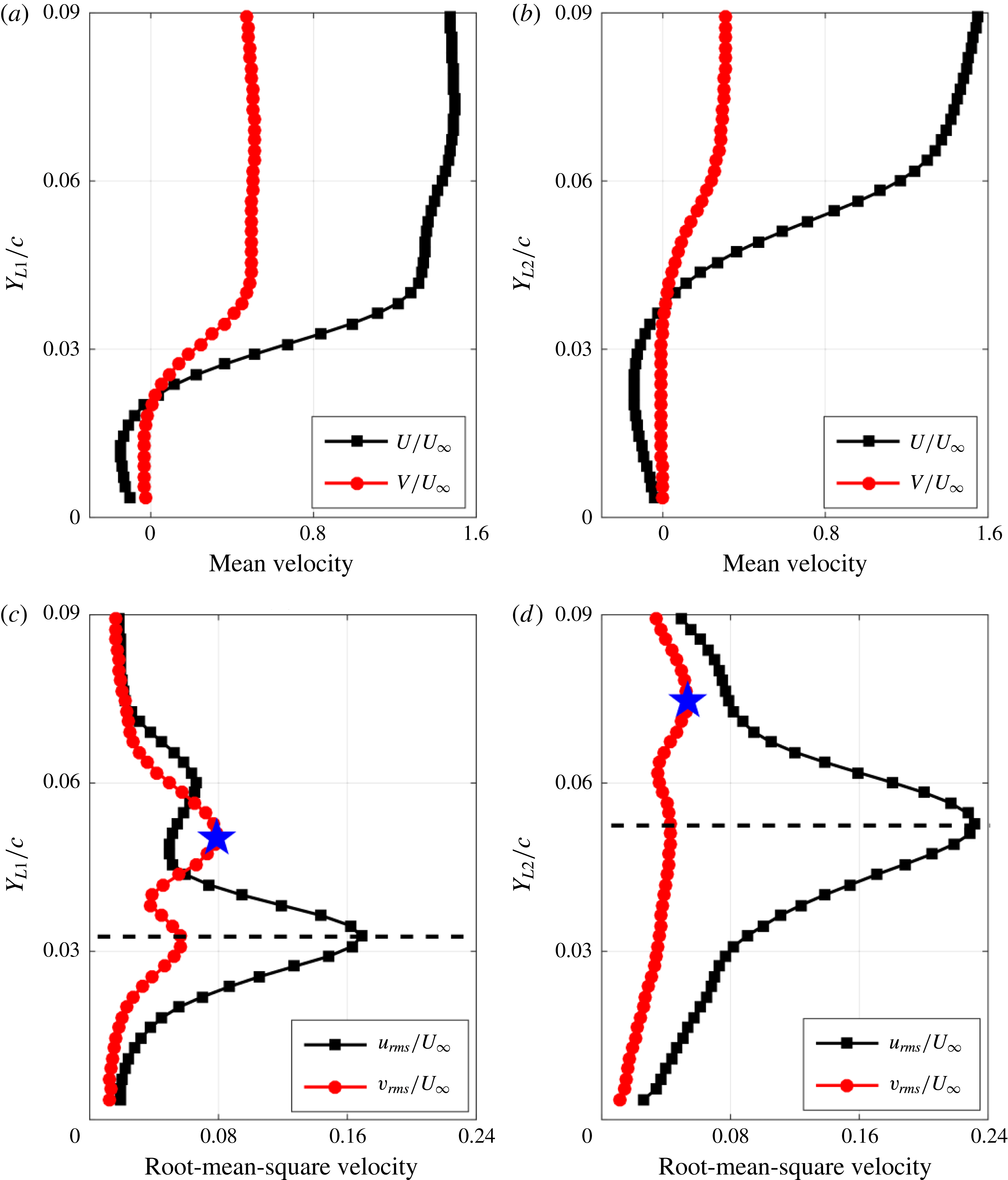
The mean velocity profiles and the root-mean-square of the velocity fluctuations extracted from the side view PIV results at
 $X/c=0.213$
and
 $X/c=0.313$
are displayed in figure 16. Mean streamwise velocity profiles (
 $U/U_{\infty }$
) in figure 16(a,b) demonstrate the classical velocity profiles of a separation bubble (Lang et al.
Reference Lang, Rist and Wagner2004; Simoni et al.
Reference Simoni, Ubaldi, Zunino, Lengani and Bertini2012; Boutilier & Yarusevych Reference Boutilier and Yarusevych2012b
). The dominant vortex core positions calculated from the Gaussian fittings are shown in figure 16(c,d) as blue pentagrams. These two vortex core positions are located at the first peaks of the two root-mean-square profiles of vertical fluctuation velocity (
 $v_{rms}/U_{\infty }$
), respectively. The coincidence between the first peak of
 $v_{rms}/U_{\infty }$
and the vortex core position indicates that the
 $v_{rms}/U_{\infty }$
band initiated from the cove in figure 17(a) is the footprint of the travelling Görtler vortices. This footprint can also be captured in figure 17(b). According to the local peaks of
 $v_{rms}/U_{\infty }$
, four virtual probes are set in the footprint (P1, P2, P3, P4 in figure 17
a) to extract the time sequences of velocity in figure 17(c). The high
 $v_{rms}/U_{\infty }$
at these virtual probe positions can be attributed to these undulatory velocity sequences. A time-shift correlation is utilized to these velocity sequences:
 $$\begin{eqnarray}R_{T}(\unicode[STIX]{x0394}t)=\frac{\overline{m_{a}(t)m_{b}(t+\unicode[STIX]{x0394}t)}}{\unicode[STIX]{x1D70E}_{m_{a}}\unicode[STIX]{x1D70E}_{m_{b}}},\end{eqnarray}$$
where
 $m_{a}$
and
 $m_{b}$
represent the velocity sequences at two different positions with the same velocity component or at the same position with different velocity components,
 $\unicode[STIX]{x1D70E}_{m_{a}}$
and
 $\unicode[STIX]{x1D70E}_{m_{b}}$
represent the standard deviation of
 $m_{a}$
and
 $m_{b}$
,
 $\overline{(\bullet )}$
denotes the average over time and
 $\unicode[STIX]{x0394}t$
denotes the time shift. The maxima of correlation coefficients (
 $R_{T}$
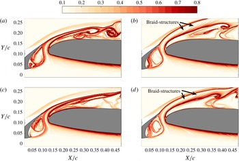
) and the time shifts are shown in figure 18. The high values of these maxima indicate that these undulatory velocity signals are highly related to the travelling motion of the Görtler vortices. The time shifts reveal that the travelling Görtler vortices pass through the measurement plane with the vortex tube slightly inclined to the plane. To further explore the physical significance of these undulatory sequences, the FTLE fields with backward integral at four characteristic instants (I1–I4 in figure 17
c) are provided in figure 19. At the trough region (I1 and I3 in figure 17
c), the ridge originating from the slat cusp converges to the ridge originating from the leading edge of the main element (figure 19
a,c). The ridge originating from the leading edge of the main element could be treated as the Lagrangian coherent structure (LCS) associated with
 $\text{SL}_{3}$
. However, at the crest region (I2 and I4 in figure 17
c), the ridge originating from the slat cusp will diverge from the ridge originating from the leading edge of the main element (figure 19
b,d). A few ridges (denoted braid structures in figure 19
b,d) emerge above the ridge originating from the leading edge of the main element. The discrepancies between figures 19(a,c) and 19(b,d) can be attributed to the travelling motion of Görtler vortices. Fixing the travelling Görtler vortices as the new reference frame (NRF), the laser sheet travels in the new reference frame. When the laser sheet cuts the DB region (shown in figure 11), the downwash motion around DB extrudes the ridge originating from the slat cusp to converge to the ridge originating from the leading edge of the main element. When the laser sheet cuts the MT region (shown in figure 11), the upwash motion between the counter-rotating vortices attracts the ridge originating from the slat cusp to diverge from the ridge originating from the leading edge of the main element. The braid structures in figure 19(b,d) are deemed to be the footprint of the upwash motion between the counter-rotating vortices. After integrating the results of figures 16–19, it could be clearly confirmed that the Görtler vortices really reside above
 $\text{SL}_{3}$
. The upwash and downwash motions associated with the travelling Görtler vortices are responsible for the undulatory velocity signals in figure 17(c). This undulatory property results in the existence of the
 $v_{rms}/U_{\infty }$
band initiated from the cove in figure 17(a).
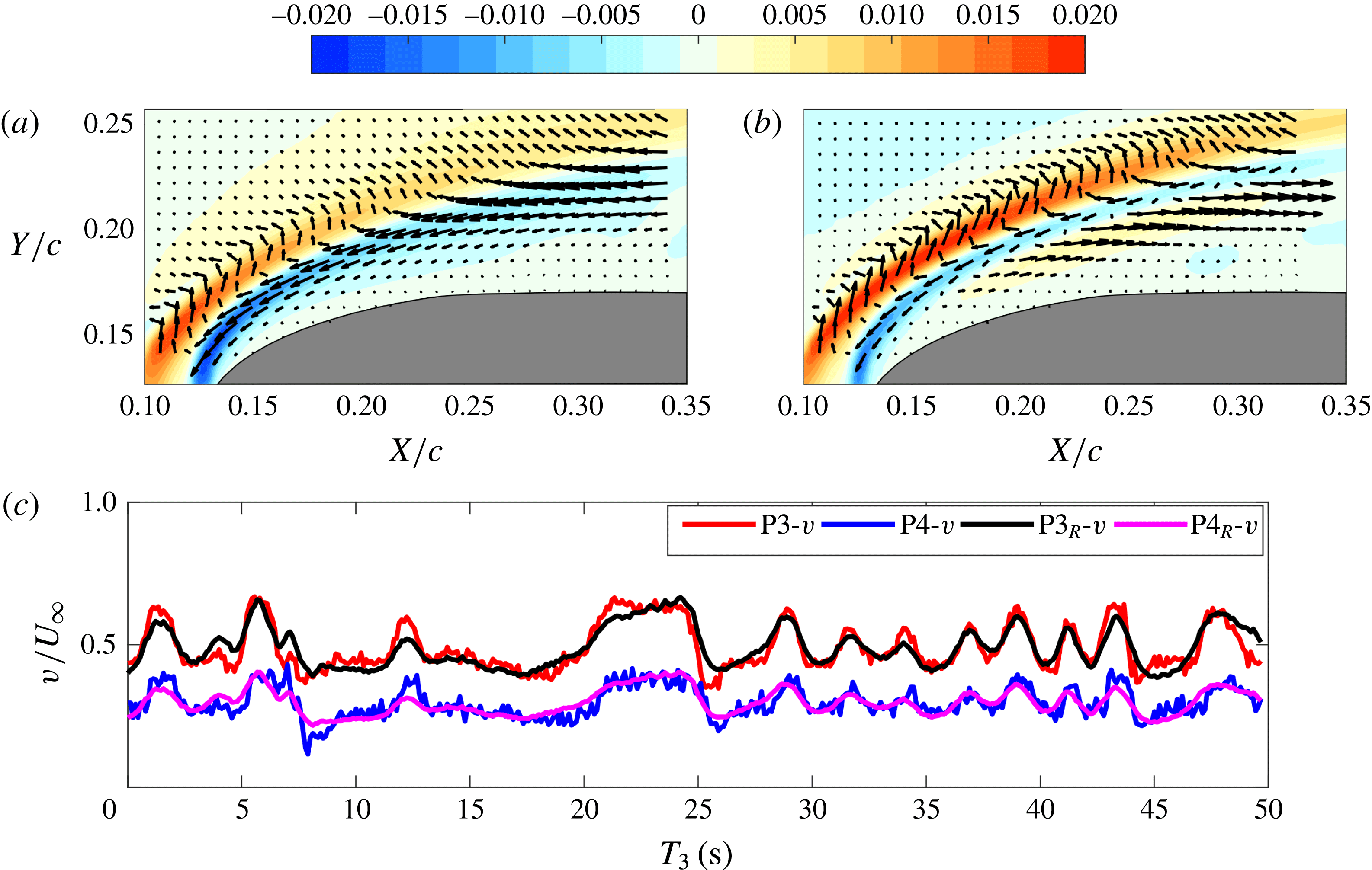
POD is applied to the fluctuation velocity field (both streamwise and vertical components) within the black box in figure 17(a). The vertical components of the first two POD modes are shown in figures 20(a) and 20(b), respectively. The velocity signals reconstructed from these two modes coincide with the original velocity signals well in figure 20(c). This accordance means that these two modes (capturing approximately 73 % of the total energy) are the most dominant modes of the flow within this region. The vertical fluctuations within the footprint of the Görtler vortices (red contour in figure 20
a,b) could represent both the upwash and the downwash motions induced by the Görtler vortices, which depend on the sign of the time coefficients of these two POD modes (Mandal & Dey Reference Mandal and Dey2011). The relative position between the Görtler vortices and the secondary counter-rotating vortices is calculated from figure 13. It is found that the second peaks of
 $v_{rms}/U_{\infty }$
in figure 16(c,d) (marked by the black dashed lines) are the footprints of the travelling secondary counter-rotating vortices. These secondary counter-rotating vortices are located within
 $\text{SL}_{3}$
. Due to the existence of the secondary counter-rotating vortices, both downwash and upwash motions exist within
 $\text{SL}_{3}$
(blue contour in figure 20
a,b). As indicated by Hain et al. (Reference Hain, Kähler and Radespiel2009), the high velocity gradient within
 $\text{SL}_{3}$
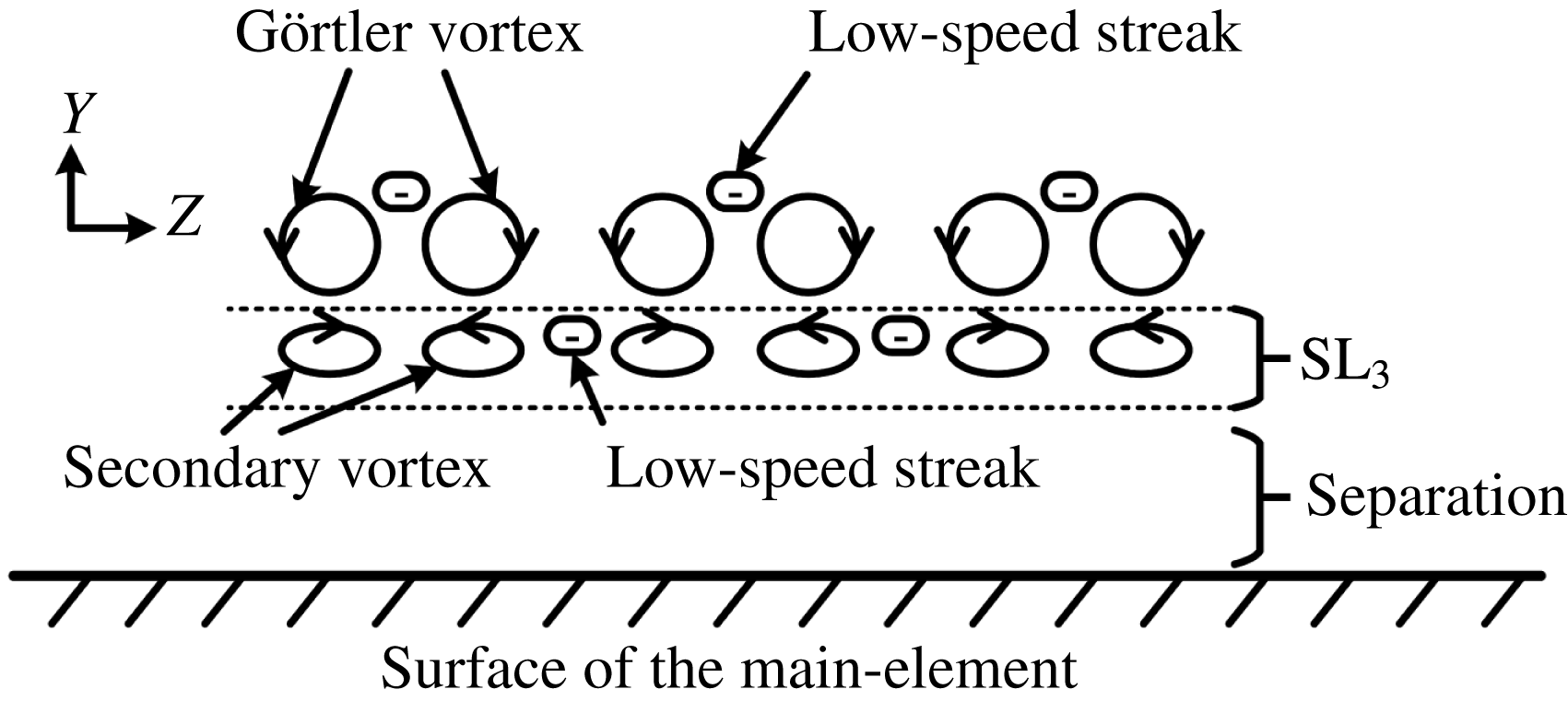
could transform the vertical fluctuations induced by the secondary counter-rotating vortices into large streamwise fluctuations. These large streamwise fluctuations could be shown as the streaky structures in figure 21. Although the velocity gradient within the slat wake could also visualize Görtler vortices as streaky structures, the streaky structures in figure 21 cannot be the representation of Görtler vortices according to the difference of the vertical positions between the Görtler vortices and the secondary counter-rotating vortices. Therefore, the travelling secondary vortices are located within
 $\text{SL}_{3}$
and generate streaky structures within
 $\text{SL}_{3}$
. This scenario is sketched in figure 22.
Both
 $v_{rms}/U_{\infty }$
and
 $u_{rms}/U_{\infty }$
contours at
 $\unicode[STIX]{x1D6FC}=16^{\circ }$
are displayed in figure 23 to show the statistical property under the absence of Görtler vortices. The
 $v_{rms}/U_{\infty }$
band initiated from the cove in figure 17(a), resulting from the travelling motion of Görtler vortices, vanishes in figure 23(a,b). The only high
 $v_{rms}/U_{\infty }$
concentrated region results from the transition of
 $\text{SL}_{3}$
. The
 $u_{rms}/U_{\infty }$
contours also demonstrate the classical transition scenario of a separated shear layer (Marxen & Henningson Reference Marxen and Henningson2011; Simoni et al.
Reference Simoni, Ubaldi, Zunino, Lengani and Bertini2012).
(a) Contour of the vertical components of the first POD mode; (b) contour of the vertical components of the second POD mode; (c) time sequences of velocity at virtual probes P3 and P4 in figure 17(a). Both the streamwise and the vertical components are shown in (a) and (b) as velocity vectors. Every fourth vector is shown for clarity. Both the original vertical velocity (red line for P3 and blue line for P4) and the vertical velocity reconstructed from the first two POD modes (black line for P3 and pink line for P4) are provided in (c).

Plane view flow visualization with volume illumination (
 $\text{FV}_{M}$
). This result captures the flow structures within
 $\text{SL}_{3}$
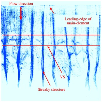
. The high-concentration regions of hydrogen bubbles (blue colour in the image) represent the low-speed streaky structures. The VS of figure 7 is marked in this figure.

Sketch of the relative positions of the Görtler vortices, the secondary counter-rotating vortex and the low-speed streak.

Root-mean-square contours of the fluctuation velocity from the PIV results at
 $\unicode[STIX]{x1D6FC}=16^{\circ }$
: (a)
 $v_{rms}/U_{\infty }$
from the PIV results focused on the gap flow; (b)
 $v_{rms}/U_{\infty }$
from the PIV results focused on the flow around the main element; (c)
 $u_{rms}/U_{\infty }$
from the PIV results focused on the gap flow; (d)
 $u_{rms}/U_{\infty }$
from the PIV results focused on the flow around the main element.

3.4 Effect of Görtler vortices on the leading-edge separated shear layer
As indicated in § 3.3, the travelling Görtler vortices could induce the travelling secondary vortices within
 $\text{SL}_{3}$
at
 $\unicode[STIX]{x1D6FC}=4^{\circ }$
. The vertical disturbances resulting from the upwash–downwash motions of these secondary vortices could generate large streamwise disturbances within
 $\text{SL}_{3}$
. These streamwise disturbances engender the scenario that the low-speed and high-speed streaks co-exist within
 $\text{SL}_{3}$
in the spanwise direction. This scenario is quite similar to the bypass transition of the separated shear layer under elevated free-stream turbulence (Mcauliffe & Yaras Reference Mcauliffe and Yaras2009). However, in the current investigation, the vortex shedding originating from
 $\text{SL}_{3}$
indicates that the modal growth associated with the K–H instability within
 $\text{SL}_{3}$
is not fully bypassed. Accordingly, the not-bypassed K–H instability is consistent with the transition of the separated shear layer under a steady three-dimensional disturbance (Lang et al.
Reference Lang, Rist and Wagner2004). In order to determine the effects of Görtler vortices on the transition process of
 $\text{SL}_{3}$
, FMD is utilized to track the growth of the disturbances within different frequency bands in this section.
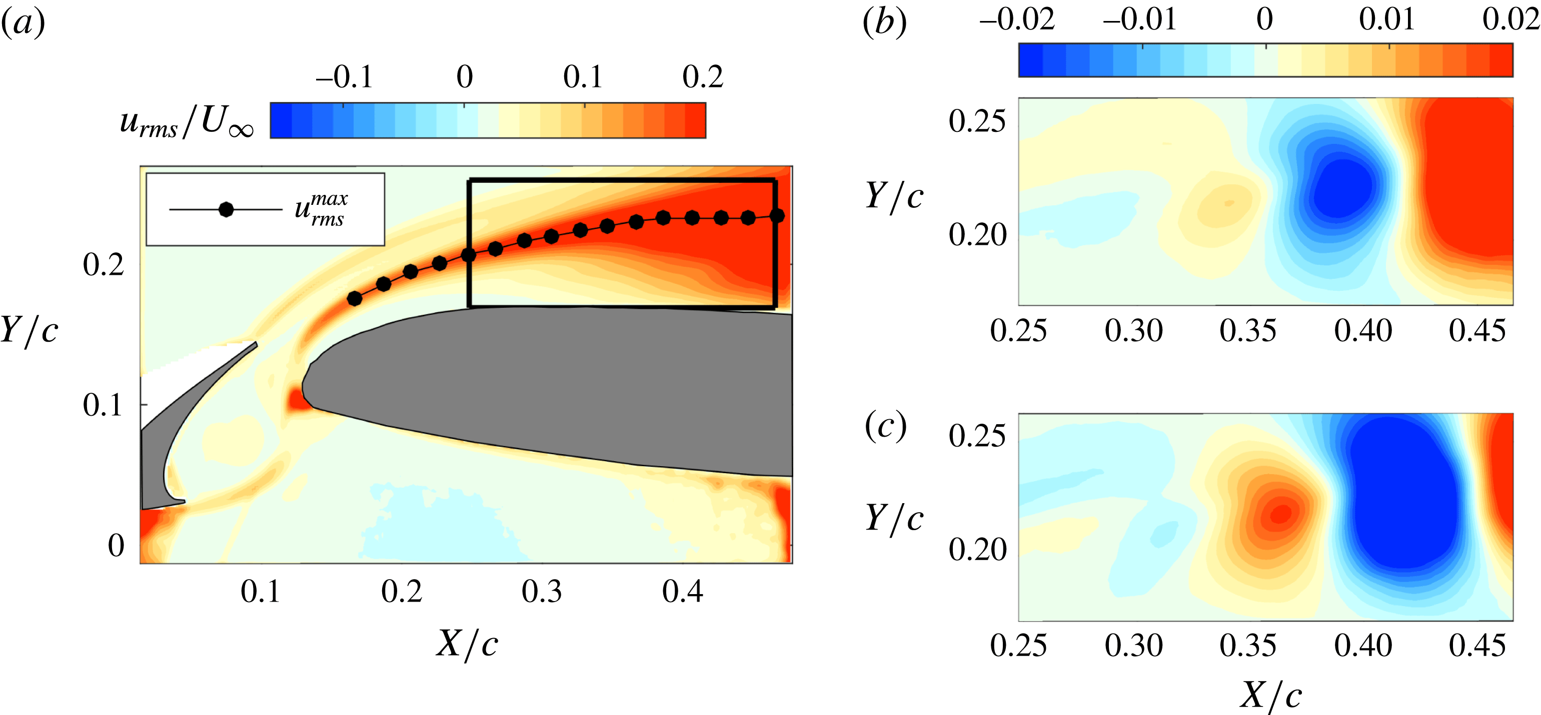
In figure 24(a), the
 $u_{rms}/U_{\infty }$
band with large amplitude is located within
 $\text{SL}_{3}$
. This is the classical scenario associated with the transition of the separated shear layer (Marxen & Henningson Reference Marxen and Henningson2011; Simoni et al.
Reference Simoni, Ubaldi, Zunino, Lengani and Bertini2012). Here, POD is utilized to the fluctuation velocity field within the black box in figure 24(a). As indicated by Lengani et al. (Reference Lengani, Simoni, Ubaldi and Zunino2014), only the vertical components are contained in POD to extract the vortex shedding phenomenon, which could eliminate the contamination from the streamwise components. The first two POD modes clearly capture the vortex shedding associated with
 $\text{SL}_{3}$
(Lengani et al.
Reference Lengani, Simoni, Ubaldi and Zunino2014).
In order to extract the frequency band associated with the vortex shedding at
 $\unicode[STIX]{x1D6FC}=4^{\circ }$
, all vertical velocity sequences in the black box (figure 24
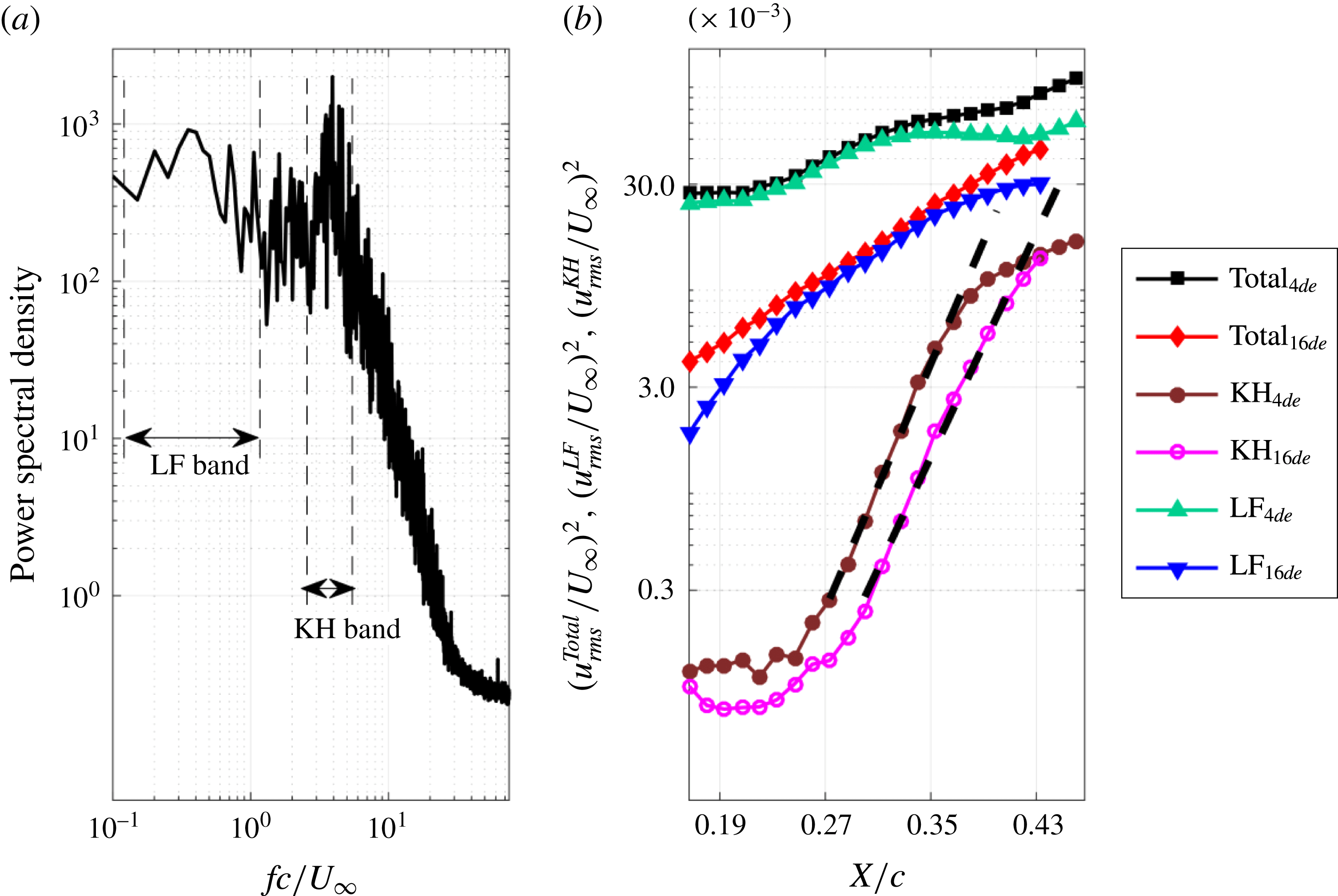
a) are contained to conduct FMD (6171 velocity sequences). The global power spectral density (PSD) within this region is shown in figure 25(a). To reconstruct the original velocity fluctuations, no window function is used for the PSD. The frequency bands associated with the low frequency fluctuations (
 $fc/U_{\infty }=0.0503{-}1.3068$
) and the K–H instability (
 $fc/U_{\infty }=2.7150{-}6.1325$
) are marked as LF band and KH band in figure 25(a), respectively. As indicated by Simoni et al. (Reference Simoni, Ubaldi, Zunino, Lengani and Bertini2012), the fluctuation energy within different frequency bands can be extracted from the power spectral density. In the current work, these two frequency bands (LF and KH) are applied to the local power spectral densities (
 $\text{PSD}_{local}$
) to track the evolution of the fluctuation energy associated with different flow structures. The
 $\text{PSD}_{local}$
of the streamwise velocity is calculated at the local peak of
 $u_{rms}/U_{\infty }$
(black line with dots in figure 24
a). The definitions of the total fluctuation energy, the KH fluctuation energy and the LF fluctuation energy are as follows:
 $$\begin{eqnarray}\displaystyle & \displaystyle (u_{rms}^{Total}/U_{\infty })^{2}=\left.\left(\unicode[STIX]{x03C0}\int _{Total}\text{PSD}_{local}(f)\,\text{d}f\right)\right/(U_{\infty })^{2}, & \displaystyle\end{eqnarray}$$
 $$\begin{eqnarray}\displaystyle & \displaystyle (u_{rms}^{KH}/U_{\infty })^{2}=\left.\left(\unicode[STIX]{x03C0}\int _{KH}\text{PSD}_{local}(f)\,\text{d}f\right)\right/(U_{\infty })^{2}, & \displaystyle\end{eqnarray}$$
 $$\begin{eqnarray}\displaystyle & \displaystyle (u_{rms}^{LF}/U_{\infty })^{2}=\left.\left(\unicode[STIX]{x03C0}\int _{LF}\text{PSD}_{local}(f)\,\text{d}f\right)\right/(U_{\infty })^{2}. & \displaystyle\end{eqnarray}$$
Finally, the spatial growth of the fluctuation energy associated with different frequency bands at
 $\unicode[STIX]{x1D6FC}=4^{\circ }$
is shown in figure 25(b). As with
 $\unicode[STIX]{x1D6FC}=4^{\circ }$
, the spatial growth of the fluctuation energy at
 $\unicode[STIX]{x1D6FC}=16^{\circ }$
is also displayed in figure 25(b). The total fluctuation energy at these two angles of attack increases along the streamwise direction. The total fluctuation energy at
 $\unicode[STIX]{x1D6FC}=16^{\circ }$
fits the exponential amplification better than that at
 $\unicode[STIX]{x1D6FC}=4^{\circ }$
. The initial value of the total fluctuation energy at
 $\unicode[STIX]{x1D6FC}=4^{\circ }$
is one order of magnitude higher than that at
 $\unicode[STIX]{x1D6FC}=16^{\circ }$
. This deviation of the initial value between these two angles of attack is mainly attributed to the deviation of LF fluctuation energy. Due to the existence of Görtler vortices at
 $\unicode[STIX]{x1D6FC}=4^{\circ }$
, the travelling secondary vortices are generated within
 $\text{SL}_{3}$
. The travelling low-speed and high-speed streaks associated with the secondary vortices could increase the low frequency disturbances within
 $\text{SL}_{3}$
in the measurement plane. As indicated by Mcauliffe & Yaras (Reference Mcauliffe and Yaras2009), these streaks could represent the potential transient growth within
 $\text{SL}_{3}$
and bypass the modal growth associated with the K–H instability. However, the similarity of the spatial growth of the KH fluctuation energy between
 $\unicode[STIX]{x1D6FC}=4^{\circ }$
and
 $\unicode[STIX]{x1D6FC}=16^{\circ }$
reveals that the K–H instability is not strongly affected by the existence of the Görtler vortices in the current investigation. Therefore, it can be concluded that the separated shear layer can be receptive to the disturbances outside the separated shear layer (generated by the Görtler vortices) to generate streaky structures. The streaky structures cannot fully bypass the modal growth associated with the K–H instability. The potential transient growth associated with the streaky structures and the modal growth associated with the K–H instability may co-exist within
 $\text{SL}_{3}$
.
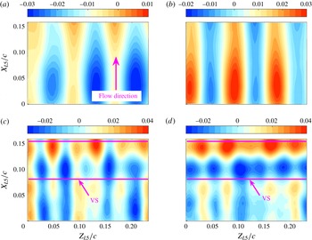
POD modes of plane view PIV measurements provide additional information on the effect of Görtler vortices on the shed vortices. Both the streamwise and the spanwise components of the fluctuation velocity are contained to obtain the POD modes. The longitudinal structures, resulting from the existence of Görtler vortices, dominate the first eight POD modes. The streamwise components of the first two POD modes are provided in figure 26(a,b) to show these longitudinal structures. As indicated by Lengani & Simoni (Reference Lengani and Simoni2015), the coherent patterns in the spanwise direction (marked VS in figure 26 c,d) represent the footprints of shed vortices associated with the K–H instability. The spanwise periodic property of these coherent patterns indicates that the shed vortices are modified by the Görtler vortices to become undulatory in the spanwise direction.
(a) Root-mean-square contour of the streamwise fluctuation velocity from the PIV results at
 $\unicode[STIX]{x1D6FC}=4^{\circ }$
; (b) first POD mode of the vertical fluctuation velocity within the black box in (a); (c) second POD mode of the vertical fluctuation velocity within the black box in (a). The local peaks of
 $u_{rms}/U_{\infty }$
are provided in (a) as black line with dots.

(a) Power spectrum density of the vertical velocity within the black box in figure 24(a); (b) spatial growth of the fluctuation energy associated with different frequency bands at
 $\unicode[STIX]{x1D6FC}=4^{\circ }$
and
 $\unicode[STIX]{x1D6FC}=16^{\circ }$
. The exponential fittings of KH fluctuation energy are marked as black dashed lines in (b).

Streamwise components of the POD modes extracted from the plane view PIV result at
 $\unicode[STIX]{x1D6FC}=4^{\circ }$
: (a) first POD mode; (b) second POD mode; (c) ninth POD mode; (d) tenth POD mode. The footprints of shed vortices are marked VS in (c) and (d). The origin of the local coordinate system is located at the bottom left corner of the field of view. The local streamwise direction and the local spanwise direction are denoted
 $X_{L5}$
and
 $Z_{L5}$
, respectively.

3.5 Origin of the Görtler vortices
In this section, the Rayleigh discriminant combined with the FV results is used to explore the origin of the Görtler vortices at
 $\unicode[STIX]{x1D6FC}=4^{\circ }$
. The position of the Görtler vortices, determined in § 3.3, also contributes to this exploration. A possible generation mechanism of Görtler vortices is proposed, which could provide evidence for the innovative generation mechanism of Inger (Reference Inger1987). Some further discussion is also given here to explain the travelling motion of Görtler vortices.
The Rayleigh discriminant applied in the current work is a modulated version (Beaudoin et al. Reference Beaudoin, Cadot, Aider and Wesfreid2004) according to the theoretical derivation (Sipp & Jacquin Reference Sipp and Jacquin2000). The formula is as follows:
 $$\begin{eqnarray}R_{D}=\frac{2\sqrt{U^{2}+V^{2}}\unicode[STIX]{x1D714}_{Z}}{K_{r}},\end{eqnarray}$$
where
 $U$
and
 $V$
represent the streamwise and the vertical components of the time-averaged velocity field, respectively. Both the spanwise vorticity
 $\unicode[STIX]{x1D714}_{Z}$
and the radius of curvature
 $K_{r}$
are calculated from the time-averaged velocity field. The formula is detailed in Beaudoin et al. (Reference Beaudoin, Cadot, Aider and Wesfreid2004). The flow in the region with positive Rayleigh discriminant is stable to the centrifugal force. Meanwhile, the region with negative Rayleigh discriminant is treated as the potential centrifugal instability region. When the stabilizing effect of viscosity cannot resist the inviscid centrifugal instability, the flow can ultimately undergo centrifugal instability.
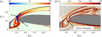
Three potential centrifugal instability regions are labelled in figure 27(a) according to the sign of the Rayleigh discriminant (
 $\text{R}_{1}$
,
 $\text{R}_{2}$
and
 $\text{R}_{3}$
in figure 27
a). For
 $\text{R}_{1}$
, the curved surface of the slat cove may lead to the occurrence of a centrifugal instability. However, if this is the case, the disturbance resulting from the centrifugal instability would modulate
 $\text{SL}_{2}$
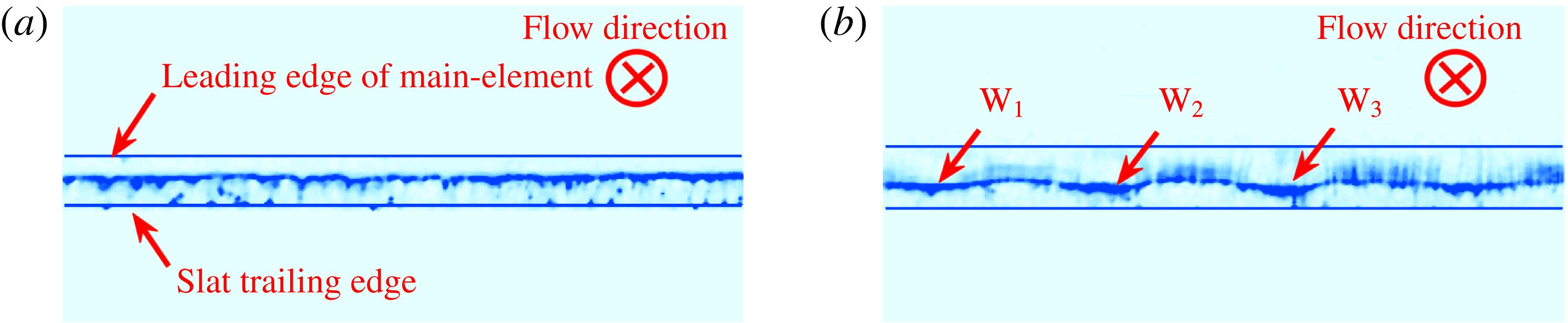
into a wavy shape in the spanwise direction. This deduction conflicts with the results of bottom view flow visualization. The hydrogen bubble curtain keeps the two-dimensional shape well at
 $Y/c=0.071$
(figure 28
a). Therefore, the flow within this potential region is finally stable to the centrifugal force. The potential centrifugal instability region
 $\text{R}_{2}$
may result from the curved streamline around the front stagnation point of the main element. As indicated by Inger (Reference Inger1987) and Marxen et al. (Reference Marxen, Lang, Rist, Levin and Henningson2009), the curved streamline above the separation point of the laminar separation bubble may play the same role as the curved wall to generate Görtler vortices. However, for the configuration with a concave wall followed with a convex wall, the convex wall could suppress the disturbance amplification resulting from the centrifugal instability around the concave wall (Benmalek & Saric Reference Benmalek and Saric1994). Therefore, with a tiny concave streamline followed with a consistent convex streamline,
 $\text{R}_{2}$
is still not deemed to be the origin region of the Görtler vortices at
 $\unicode[STIX]{x1D6FC}=4^{\circ }$
. For
 $\text{R}_{3}$
, the potential centrifugal instability region is located around the upper right boundary of
 $\text{SB}_{S}$
. The wavy pattern of the hydrogen bubble curtain at
 $Y/c=0.126$
(
 $\text{W}_{1}$
,
 $\text{W}_{2}$
and
 $\text{W}_{3}$
in figure 28
b) strongly indicates that
 $\text{R}_{3}$
is responsible for the generation of the centrifugal instability. Figure 19(b) is revisited in figure 27(b) superimposed by the instantaneous streamlines. Since the ridge within the FTLE field can be regarded as the virtual boundary (Shadden et al.
Reference Shadden, Lekien and Marsden2005), the ridge enclosed
 $\text{SB}_{S}$
can be treated as a virtual curved boundary. This virtual curved boundary could be approximated by a special streamline, which splits the slat cove bubble and the gap flow. This special streamline based on the averaged velocity is marked in figure 27(a) as a black line. Around the slat cove, the free-stream flow will suffer from a virtual convex boundary followed with a virtual concave boundary. The centrifugal instability could be generated in the concave region
 $\text{R}_{3}$
. Since the centrifugal instability is generated from the virtual curved wall, the counter-rotating vortices are named ‘Görtler vortices’. It should be emphasized that the Rayleigh discriminant is based on the two-dimensional basic flow. Therefore, only the Rayleigh discriminant concentrated at the flow regions with small spanwise disturbances can make sense. Fortunately, this limitation does not affect the determination of the origin of Görtler vortices in the current investigation.
(a) Contour of Rayleigh discriminant; (b) revisiting of figure 19(b). A special black streamline calculated from the averaged flow is superimposed on (a). The streamlines calculated from the instantaneous flow are superimposed on (b).

Bottom view FV results: (a)
 $Y/c=0.071$
; (b)
 $Y/c=0.126$
. The main flow direction points inside of the measurement plane.

Side view FV results at
 $\unicode[STIX]{x1D6FC}=4^{\circ }$
. The shadows of VT appear in (a) and (b) by image enhancement. The nomenclatures MT, VT and DB are same as those in figure 11. The nomenclatures
 $\text{SB}_{S}$
and RP are same as those in figure 7. The superposition among (a), (b) and (c) is shown in (d).

Side view flow visualization can provide additional evidence for the origin of Görtler vortices. Benefiting from the application of the horizontal hydrogen bubble curtain, the three-dimensional flow structures outside the laser sheet can still be illuminated by the scattered light of the hydrogen bubble inside the laser sheet. Following the definition of NRF, when the laser sheet cuts the MT or the DB region (shown in figure 11), a shadow of VT will be projected into the laser sheet plane (VT in figure 29
a,b). In figure 29(c), the laser sheet just passes the VT. The relative positions of MT, VT and DB in side view FV are clearly manifested in figure 29(d). These relative positions are consistent with the end view FV results. It deserves to be paid more attention to the fact that the vortex tube of the Görtler vortices emanates from the upper right boundary of
 $\text{SB}_{S}$
. This phenomenon is consistent with the result in figure 17(a) that the footprint of the travelling Görtler vortices initiates from the upper right boundary of
 $\text{SB}_{S}$
. In figure 30(a), the diverging averaged streaky line still initiates from
 $\text{R}_{3}$
(after arrow 1). The dissipation of the streaky line could represent the amplification of the disturbances associated with the centrifugal instability. In this view, the initial amplification of the disturbances emerges in
 $\text{R}_{3}$
at
 $\unicode[STIX]{x1D6FC}=4^{\circ }$
. After passing through the gap region, the disturbances are strongly amplified. On the contrary, for the case without Görtler vortices (
 $\unicode[STIX]{x1D6FC}=16^{\circ }$
), the diverging averaged streaky line emerges after arrow 2 in figure 30(b). This diverging pattern can be ascribed to the occurrence of RP.
Averaged side view FV results: (a)
 $\unicode[STIX]{x1D6FC}=4^{\circ }$
; (b)
 $\unicode[STIX]{x1D6FC}=16^{\circ }$
. A total of 4500 FV snapshots are utilized for the averaged process at these two angles of attack.

It should be emphasized that the wavy pattern in figure 28(b) also travels in the spanwise direction. The downstream travelling Görtler vortices stick to the travelling wavy pattern. Therefore, the travelling property of the Görtler vortices is just an inheritance of the travelling property of the wavy pattern in
 $\text{R}_{3}$
. As indicated in the open cavity flow (Faure et al.
Reference Faure, Adrianos, Lusseyran and Pastur2007, Reference Faure, Pastur, Lusseyran, Fraigneau and Bisch2009; Faure Reference Faure2014; Douay et al.
Reference Douay, Pastur and Lusseyran2016a
; Douay, Lusseyran & Pastur Reference Douay, Lusseyran and Pastur2016b
), the separation bubble within the slat cove could contain a spanwise travelling flow. This travelling flow could drive the wavy pattern to travel in the spanwise direction.
3.6 Discussion
Inger (Reference Inger1987) suggested that the concave streamline above the separation point of the separation bubble could replace the concave wall to generate Görtler vortices. However, it is not the case in these investigations with a laminar separation bubble (Watmuff Reference Watmuff1999; Hain et al. Reference Hain, Kähler and Radespiel2009; Simoni et al. Reference Simoni, Ubaldi, Zunino, Lengani and Bertini2012; Boutilier & Yarusevych Reference Boutilier and Yarusevych2012b ; Kurelek et al. Reference Kurelek, Lambert and Yarusevych2016). Therefore, in this section, modified criteria for the generation of Görtler vortices with a curved streamline are proposed according to the primary theoretical results of Inger (Reference Inger1987). The results in the current investigation combined with the results from the literature are deliberated to support these modified criteria:
-
(I) A stable instantaneous virtual concave boundary with the vorticity distribution meeting the negative Rayleigh discriminant.
-
(II) The curvature of the instantaneous virtual boundary must be high enough to generate strong centrifugal instability to survive from the stability effect of viscosity.
The investigation on the backward-facing step of Beaudoin et al. (Reference Beaudoin, Cadot, Aider and Wesfreid2004) is the only experimental evidence to support the existence of Görtler vortices after the laminar reattachment point of the backward-facing step. This phenomenon can be explained by the modified criteria. The laminar reattachment provides a stable instantaneous virtual concave boundary around the reattachment point. The Rayleigh discriminant reveals that the potential centrifugal instability region around the reattachment point is the origin of the Görtler vortices (Beaudoin et al.
Reference Beaudoin, Cadot, Aider and Wesfreid2004). However, the classical sketch of the flow over the backward-facing step reveals that Görtler vortices are not the dominant coherent structures (Simpson Reference Simpson1989). K–H instability dominates the initial transition process of the separated shear layer. The separation bubble is formed by the turbulent reattachment of the separated shear layer. This no Görtler vortices scenario can also be explained by the modified criteria. The shed vortices originating from the K–H instability and the following rapid breakdown make the instantaneous virtual boundary around the reattachment chaotic. Therefore, criterion I is violated in the turbulent reattachment case. For the results at
 $\unicode[STIX]{x1D6FC}=0^{\circ }$
in the current investigation, although the curved streamlines exist in the time-averaged gap flow (figure 5
a), the chaotic vortex structures within the gap flow still make the instantaneous virtual boundary unsteady and disorganized. These chaotic instantaneous virtual boundaries also violate criterion I and prevent the occurrence of regular Görtler vortices.
Inger (Reference Inger1987) indicated that Görtler instability should always occur around the separation point of the laminar separated shear layer. However, it is not the case in these investigations with the laminar separation bubble (Watmuff Reference Watmuff1999; Hain et al.
Reference Hain, Kähler and Radespiel2009; Simoni et al.
Reference Simoni, Ubaldi, Zunino, Lengani and Bertini2012; Boutilier & Yarusevych Reference Boutilier and Yarusevych2012b
; Kurelek et al.
Reference Kurelek, Lambert and Yarusevych2016). The unfitness for criterion II is treated as the reason for this no Görtler vortices scenario. Though the stable instantaneous virtual concave boundary exists around the separation point of the laminar separation bubble, the curvature of the virtual boundary is insufficient to generate strong centrifugal instability to survive from the stability effect of viscosity. This unfitness for criterion II also contributes to the no Görtler vortices scenario at
 $\unicode[STIX]{x1D6FC}=14^{\circ }{-}16^{\circ }$
in the current investigation. Though criterion I is met at
 $\unicode[STIX]{x1D6FC}=14^{\circ }{-}16^{\circ }$
, the curvature of the virtual boundary at
 $\unicode[STIX]{x1D6FC}=16^{\circ }$
is weaker than that at
 $\unicode[STIX]{x1D6FC}=4^{\circ }$
(comparing figure 9 with figure 7) qualitatively. Therefore, both the two criteria should be met to generate Görtler vortices by a virtual curved boundary.
It should be emphasized that these two criteria only make sense qualitatively. The leading edge of the main element also affects the flow within the gap region. This complex geometry makes it hard to provide quantitative criteria. Therefore, follow-up investigations with simplified experimental configurations should be conducted to verify that these two criteria are quantitative. Meanwhile, the no-slip condition is not met on the virtual curved boundary. Therefore, it is normal to find a few differences between the characteristics of the Görtler vortices generated from the virtual boundary and those generated from the real curved wall.
4 Conclusion
The low-Reynolds-number flow over a multi-element airfoil (30P30N) has been investigated with time-resolved particle image velocimetry (TR-PIV) and flow visualization (FV). According to the evolution of dominant flow structures around the main element with angle of attack, three regimes can be classified in the current work. The dominant coherent structures in these regimes are different from the classical coherent structures around the multi-element airfoil at high Reynolds numbers (
 $Re_{c}=10^{6}{-}10^{7}$
).
-
(i) At
$\unicode[STIX]{x1D6FC}=0^{\circ }$
, irregular streamwise vortices exist above the main element. The shear layer originating from the lower surface of the slat cannot pass through the gap region and results in abundant vortex structures around the gap region. The stretch effect within the gap flow may deform these vortex structures into the irregular streamwise vortices above the main element. -
(ii) At
$\unicode[STIX]{x1D6FC}=2^{\circ }{-}12^{\circ }$
, regular Görtler vortices with a travelling property exist above the main element. In this regime, the separated shear layer originating from the lower surface of the slat can pass through the gap region and reattaches on the slat cove surface to form the slat cove separation bubble. The position of the Görtler vortices and the Rayleigh discriminant are combined to reveal that the upper right boundary of the slat cove separation bubble (virtual curved boundary layer) could play the role as real curved wall to generate regular Görtler vortices. The spanwise travelling flow within the slat cove separation bubble could drive those Görtler vortices to travel in the spanwise direction by affecting the virtual curved boundary. Meanwhile, the relative position between the Görtler vortices and the separated shear layer originating from the leading-edge separation of the main element results in complex interactions between these two structures. The secondary counter-rotating vortices induced by Görtler vortices exist within the separated shear layer and could generate streaky structures. Finally, the potential transient growth associated with the streaky structures and the modal growth associated with the K–H instability could co-exist within the separated shear layer. -
(iii) At
$\unicode[STIX]{x1D6FC}=14^{\circ }{-}16^{\circ }$
, neither irregular streamwise vortices nor Görtler vortices exists above the main element. The separated shear layer originating from the lower surface of the slat can still pass through the gap region. The laminar reattachment of the separated shear layer still forms the slat cove separation bubble. However, the curvature of the upper right boundary of the slat cove separation bubble may not be strong enough to generate Görtler vortices.


After generalizing the results both in the current work and in the literature, modified criteria for generating Görtler vortices by virtual curved boundary are proposed. Both stable instantaneous virtual curved boundary and strong curvature are necessary for the generation of Görtler vortices. This qualitative criterion still needs to be verified by follow-up work with a simplified experimental configuration.
Acknowledgements
This work is supported by the National Natural Science Foundation of China (11327202, 11721202) and the Fundamental Research Funds for Central Universities (YWF-16-JCTD-A-05).