





1 Introduction
Latent variable models such as confirmatory factor analysis (CFA) and structural equation modeling (SEM) explain associations among observed variables, contained in the mean zero
$p$
 -dimensional vector
$x$
 , by positing the existence of unobserved latent variables, contained in the
$k$
 -dimensional vector
$f$
 with
$k \leq p$
 , that linearly affect the observed variables.
Consider the confirmatory factor model with free parameters contained in the vector
$\theta $
 , whose model-implied covariance matrix has the form

Here,
$\Lambda (\theta )$
 is a
$p \times k$
 loading matrix, and
$\Phi (\theta )$
 and
$\Psi (\theta )$
 are covariance matrices of dimensions
$k \times k$
 and
$p \times p$
 , respectively (see Bollen, Reference Bollen1989, for a textbook introduction). We will assume that the model is identified, which rules out exploratory factor analysis.
The main motivation for the covariance model in eq. (1) is that if

where
$f$
 and
$u$
 are uncorrelated, have zero mean, and respective covariance matrices
$\Phi $
 and
$\Psi $
 , then

The problem of factor indeterminacy is that there exist infinitely many
$(f,u)$
 -pairs that fulfill eq. (2) and have the required mean and covariances (e.g., Guttman, Reference Guttman1955; Krijnen et al., Reference Krijnen, Dijkstra and Gill1998; McDonald, Reference McDonald1974; Mulaik, Reference Mulaik1976). Factor indeterminacy has a long and complicated history (see Mulaik, Reference Mulaik2009, Section 13.4 and Steiger, Reference Steiger1979, for an overview).
The present article investigates the role of factor indeterminacy in simulation studies and in linear SEM. Based on our analysis, we give practical recommendations for designing simulation studies that take factor indeterminacy into account. We revisit factor indeterminacy in Section 2. Section 3 considers how taking indeterminacy into account affects the interpretation of simulation studies. Our main finding is that a single simulation study represents a larger class of equivalent studies. One consequence is that simulating manifest variables from a model-implied covariance matrix always supports a plethora of latent variables. Section 4 shows how the functional form of a covariance-based linear SEM is unidentified as a consequence of indeterminacy, leaving open the possibility of curvilinear factor relations that violate the linear trends typically assumed in the SEM specification. Section 5 examines factor indeterminacy under additional constraints, with technical details relegated to Appendix A. We there focus on independence between common and unique factors, the causal interpretation of linear SEM, and simulation studies comparing factor scores. Section 6 gives practical recommendations for conducting simulation studies and for studies examining the performance of factor scores. Section 7 provides numerical illustrations of our findings.
In addition to Appendix A, there is a Supplementary Material that contains the remaining proofs and additional derivations. R (R Core Team, 2020) code for the numerical illustrations is available on the Open Science Framework at this repository: https://osf.io/2jgvb/overview?view_only=b0dafeb5f31b438ab30f6ee38d7cfa67. We let
$|\cdot |$
 indicate the Euclidean norm, and let
$u'$
 denote the transpose of a vector
$u$
 .
We occasionally state that an assumption must be known through substantive means, meaning it relies on domain theory rather than purely statistical evidence. A related concept is that of a partly testable hypothesis, meaning a hypothesis that has some testable implications, but where even if all testable implications of the hypothesis hold, it need not be the case that the hypothesis holds (for a formal definition, see Section 1 of the Supplementary Material).
2 Revisiting factor indeterminacy
Guttman (Reference Guttman1955, p. 66) showed that there always exist
$f$
 and
$u$
 such that eq. (2) holds, but added that the existence problem had “too many affirmative answers.” While Guttman (Reference Guttman1955) made no probabilistic assumptions in his arguments, we assume that
$x$
 is a random vector, and so also
$(f,u)$
 is a random vector.
We assume that the covariance model in eq. (1) is correctly specified and identified, and that the factors and error terms do not have perfect linear dependence, which simplifies some of our upcoming arguments.
Assumption 1.
-
(1) (Identification and correct covariance model specification) There is a unique $\theta _0$
 such that
$\Sigma (\theta _0) = \Sigma ,$
where
$\Sigma = \operatorname {Cov} \, (x)$
and
$\Sigma (\theta )$
is defined in eq. (1).
-
(2) (Regularity) The matrices $\Phi := \Phi (\theta _0)$
and
$\Psi := \Psi (\theta _0)$
are positive definite, and
$\Lambda = \Lambda (\theta _0)$
has full column rank. -
(3) We have $ \operatorname {E} x = 0$
.


Under this assumption, we may consider
$\Lambda , \Phi , \Psi $
 as given.
Definition 1. Suppose that eq. (3) holds for the given matrices
$\Lambda , \Phi , \Psi $
 . Suppose further that
$f$
 and
$u$
 are uncorrelated and zero mean random vectors of dimensions
$k$
 and
$p$
 , respectively. We call the
$(f,u)$
 -pair admissible for x if
$x = \Lambda f + u$
 ,
$ \operatorname {Cov} \, (f) = \Phi $
 and
$ \operatorname {Cov} \, (u) = \Psi $
 .
The class of admissible
$(f,u)$
 -pairs is infinite (e.g., Guttman, Reference Guttman1955; McDonald, Reference McDonald1974), and its characterization is part of classical psychometric theory. We here present a simple and self-contained characterization using the classical Thurstone–Thomson regression predictor (Thomson, Reference Thomson1934; Thurstone, Reference Thurstone1935)

where
$\Sigma $
 is invertible under Assumption 1. In general (even when
$\Sigma $
 is singular), this predictor is the unique best affine predictor of
$f$
 (see Section 3 of Neudecker & Satorra, Reference Neudecker and Satorra2003). Therefore, its residual

will have zero mean and will be uncorrelated with
$x$
 (for a proof, see Lemma 1 in the Supplementary Material). Its covariance matrix is the mean square error (MSE) matrix of the regression predictor
$Tx$
 :

When
$\Sigma $
 is singular,
$\Sigma ^{-1}$
 may be replaced by a generalized inverse (Neudecker & Satorra, Reference Neudecker and Satorra2003, Section 3).
Now suppose we do not know whether there exist
$f$
 and
$u$
 that together generate
$x$
 according to eq. (2). We may attempt to construct such
$f$
 and
$u$
 by generating a
$k$
 -dimensional vector
$y$
 that fulfills the above properties of the residual.
Definition 2. A
$k$
 -dimensional random vector
$y$
 that has zero mean and is uncorrelated with
$x$
 is called a Thurstone residual if
$ \operatorname {Cov} \, (y) = \text {MSE}$
 .
Given a Thurstone residual, we may define
$f = T x + y$
 and
$u = x - \Lambda f = (I_p - \Lambda T)x - \Lambda y$
 , so that eq. (2) holds. The following proposition states that this produces an admissible
$(f,u)$
 -pair, and that all admissible pairs are formed in this manner.
Proposition 1. Suppose Assumption 1 holds.
-
(i) Assume $y$
is a Thurstone residual. Define (6) $$ \begin{align} f = Tx + y, \qquad u = \left(I_p - \Lambda T \right) x - \Lambda y. \end{align} $$
Then $(f,u)$
is admissible for
$x$
. -
(ii) Conversely, suppose $(f,u)$
is admissible for
$x$
. Then eq. (6) holds with
$y = f - Tx$
, and
$y$
is a Thurstone residual.


Proposition 1(i) has a Hilbert-space geometric interpretation known as the “factor cone” (see Mulaik, Reference Mulaik1976).
The following corollary gives a sharp distribution-free tail bound for the discrepancy between the factors
$f_1$
 and
$f_2$
 in two admissible pairs
$(f_1, u_1)$
 and
$(f_2, u_2)$
 for
$x$
 in terms of the trace of the MSE. It follows by Markov’s inequality and complements earlier characterizations of the latent factor space (e.g., Guttman, Reference Guttman1955, Theorem 3).
Corollary 1. Suppose Assumption 1 holds. Suppose we are given two admissible
$(f,u)$
 -pairs for
$x$
 , with factors
$f_1$
 and
$f_2$
 , on the same probability space. Then, for any
$\epsilon> 0$
 , we have the following sharp bound:

Moreover,
$\operatorname *{\mathrm {Tr}}( \mathrm {MSE}) = \sum _{i=1}^k \Phi _{i,i} (1 - \rho _i^2)$
 , where
$\rho _i = \operatorname {\mathrm {Cor}}((Tx)_i,(f)_i)$
 and
$(f)_i$
 is the
$i$
 th coordinate of any admissible factor
$f$
 .
The squared correlations
$\rho _i^2$
 between the Thurstone factor score and the factor are reasonable and well-known measures of factor score performance (Mulaik, Reference Mulaik2009, Chapter 13.3). Yet Corollary 1 is general and concerns the space of admissible factors. Therefore, Corollary 1 shows that the justification of
$\rho _i^2$
 as a measure for factor indeterminacy is not limited to linear factor scores, but is a foundational aspect of factor indeterminacy. In an empirical investigation,
$\operatorname *{\mathrm {Tr}}( \mathrm {MSE})$
 would need to be computed based on estimated parameters, as is standard in the above-mentioned measures of factor indeterminacy. An implication of the sharpness of the bound in Corollary 1 is that for all
$0 < \epsilon \leq 2 \sqrt {\operatorname *{\mathrm {Tr}}( \mathrm {MSE})}$
 , there exist factors
$f_1, f_2$
 whose distance is at least
$\epsilon $
 with probability
$1$
 .
The MSE matrix of eq. (5) has been widely studied (Guttman, Reference Guttman1955; Krijnen, Reference Krijnen2004, Reference Krijnen2006a, Reference Krijnen2006b; Schneeweiss & Mathes, Reference Schneeweiss and Mathes1995; Williams, Reference Williams1978). This body of research identifies conditions under which the MSE converges to zero when
$p$
 increases. The MSEs of other linear factor estimators are upper bounds for the MSE of the Thurstone factor score, as
$Tx$
 is the best affine predictor of
$f$
 (Neudecker & Satorra, Reference Neudecker and Satorra2003), and therefore conditions under which the MSE of, for example, Bartlett scores converges to zero (see, e.g., Grønneberg & Irmer, Reference Grønneberg and Irmer2024, Section 2.1) also imply that the MSE matrix of eq. (5) converges to zero. Under these additional conditions, Corollary 1 then shows that factor indeterminacy vanishes as
$p$
 increases.
3 Factor indeterminacy in simulation studies
Monte Carlo studies are prevalent in psychometric methodological research as a tool to investigate estimation and goodness-of-fit procedures in finite-sample settings across a range of distributional conditions. In the following, we distinguish between two approaches to simulating data and show how factor indeterminacy broadens the conventional interpretation of a simulation condition.
When simulating factor models, we may either simulate
$x$
 directly, which we call Approach 1, or first simulate
$(f,u)$
 and generate
$x$
 from eq. (2), which we call Approach 2. In the following, we interpret how factor indeterminacy influences these two simulation approaches.
3.1 Approach 1: Simulating the manifest variables
A common approach when conducting a simulation study for factor modeling is to fix the model parameters contained in
$\Lambda $
 ,
$\Phi ,$
 and
$\Psi $
 to values reminiscent of those found in empirical research. Then, the model-implied covariance matrix
$\Sigma $
 of
$x$
 is calculated by eq. (3). Random samples are then drawn from a distribution whose covariance matrix equals
$\Sigma $
 (e.g., methods such as Foldnes and Grønneberg, Reference Foldnes and Grønneberg2022b, Foldnes and Olsson, Reference Foldnes and Olsson2016, Grønneberg and Foldnes, Reference Grønneberg and Foldnes2017, Grønneberg et al., Reference Grønneberg, Foldnes and Marcoulides2022, Mair et al., Reference Mair, Satorra and Bentler2012, and Vale and Maurelli, Reference Vale and Maurelli1983).
Many simulation methods offer additional control of features of
$x$
 , the manifest vector, thus allowing the simulated data to match certain aspects of real-world data such as marginal skewness and kurtosis. Controlling features of
$x$
 comes at the cost of loss of control over the distributions of
$f$
 and
$u$
 . Consider, for instance, the well-known Vale and Maurelli (Reference Vale and Maurelli1983) simulation method, which is the default non-normal simulation method in the R (R Core Team, 2020) package lavaan (Rosseel, Reference Rosseel2012), and generates
$x$
 by coordinate-wise application of third-degree polynomials to a multivariate normal random vector. Initially, it is not even clear that an admissible
$(f,u)$
 -pair exists for an
$x$
 vector generated by Vale–Maurelli. That is, one might worry that no
$(f,u)$
 -pair exists that can generate the distribution of
$x$
 through eq. (2). Fortunately, Proposition 1 ensures that admissible
$f$
 and
$u$
 exist, so the simulated
$x$
 can always be embedded in the factor model (2).
Moreover, admissibility is not unique: the same
$x$
 admits a continuum of
$(f,u)$
 -pairs. Thus, what is typically treated as a single simulation condition in fact represents a set of latent conditions, spanning many possible joint distributions of
$f$
 and
$u$
 consistent with the simulated manifest data.
In theory, it could be that the class of
$(f,u)$
 -pairs only had members with highly unrealistic distributions. To make sure this does not happen, we may inspect some of the possible
$(f,u)$
 -pairs. We can do this by generating a random vector
$(x',y')'$
 with the covariance matrix given by Proposition 1, and then computing
$f$
 and
$u$
 using the formulas in Proposition 1. Methodologically, this simulation problem has the same structure as simulating
$x$
 : Instead of just simulating
$x$
 with a fixed covariance matrix, we simulate the augmented variable
$(x',y')'$
 that fulfills the covariance restrictions given by Proposition 1. For example, we may simulate
$(x', y')'$
 using the simulation method of Foldnes and Olsson (Reference Foldnes and Olsson2016), where
$x$
 and
$y$
 are constrained to be uncorrelated and to have the required covariance matrices. We illustrate this process in Section 7.1.
3.2 Approach 2: Simulating the latent variables
In this approach, one specifies a joint distribution for
$(f,u)$
 satisfying at least
$ \operatorname {E} [f]=0$
 ,
$ \operatorname {E} [u]=0$
 ,
$ \operatorname {E} [fu']=0$
 ,
$ \operatorname {Cov} \, (f)=\Phi $
 , and
$ \operatorname {Cov} \, (u)=\Psi $
 , and then generates manifest observations through
$x=\Lambda f+u$
 (e.g., Du & Bentler, Reference Du and Bentler2022; Jiang & Yuan, Reference Jiang and Yuan2017). It is natural to think about the
$(f,u)$
 -pair used in the simulation as the true latent variables of the resulting
$x$
 .
For any manifest
$x$
 , Proposition 1 shows that there is a large class of admissible decompositions
$(f,u)$
 that generate the same manifest vector according to (2). The specific pair used during simulation is one element of this admissible class, but it is not singled out by the manifest data. Both numerically and in terms of the distribution of the manifest variables, all admissible solutions are therefore on an equal footing, possibly excepting solutions that violate properties known by the users of the statistical methods tested under simulation, see the technical discussion in Appendix A.5.
In a statistical investigation, only the manifest variables are available, and therefore any statistical investigation emulated in a simulation study may be considered as a function of the distribution of the manifest variables alone. Simulating from the equations induces a distribution on
$x$
 which we could draw directly from, positioning Approach 2 as being an instance of Approach 1.
Yet, an important difference between the direct and the equation-based simulation approaches is that the class of possible
$(f,u)$
 -pairs which could have generated
$x$
 is in the latter approach known to include the original
$(f,u)$
 -pair. This pair can be constructed to fulfill desirable properties, such as linear trends among the coordinates of
$f$
 as required by linear SEM (see Section 4). In contrast, simulating
$x$
 directly does not control any properties of
$(f,u)$
 except those guaranteed by Proposition 1, and identifying whether any
$(f,u)$
 -pair that can generate
$x$
 has desirable properties may be difficult to establish.
4 Factor indeterminacy in linear SEM
SEM is based on factor analysis and is therefore affected by the factor indeterminacy problem. While SEM and factor indeterminacy have been discussed earlier, such as in Vittadini (Reference Vittadini1989) and in the textbook by James et al. (Reference James, Mulaik and Brett1982, pp. 164–167), we here focus on how factor indeterminacy influences trend specification in linear SEM, which, as far as we can tell, has not been adequately discussed in the literature.
We restrict attention to mean-centered linear SEM, whose parameters are identified via the covariance matrix of the observations (for a textbook treatment, see Bollen, Reference Bollen1989). Factor indeterminacy also influences trend identification in non-linear SEM, but we do not consider this case in the present article, since parameter identification in non-linear SEM depends not only on the mean and covariance structure of the observations (Wall & Amemiya, Reference Wall and Amemiya2001).
Suppose
$\Phi $
 follows the restrictions of an identified path model, so that the covariance matrix of
$x$
 is of the form assumed in linear SEM. Often, this is seen as sufficient for considering a linear SEM correctly specified. But the standard interpretation of the parameters of a linear SEM rests on a foundational, though often neglected, assumption that the associations between the exogenous
$\xi $
 factors and the endogenous
$\eta $
 variables are linear. In econometrics, this linearity is explicitly assumed by conditions, such as
$ \operatorname {E} [\zeta | \xi ] = 0,$
 where
$\zeta $
 is the error term of the system (see Greene, Reference Greene2012, Chapter 10.6.5 and Chipman, Reference Chipman2013, Chapter 8). In psychometrics, this assumption is often not made explicitly, and we will see that it is not guaranteed to hold.
Such linearity does not follow from covariance assumptions alone (a nice illustration of this is Mooijaart and Satorra, Reference Mooijaart and Satorra2009). Therefore, non-linear associations between
$\xi $
 and
$\eta $
 are allowed under Assumption 1. This is illustrated in an upcoming numerical example where we show that the space of possible
$(f,u)$
 -pairs that can generate
$x$
 contains highly non-linear associations, even when
$x$
 is exactly normal.
We now show how to connect our previous analysis with a linear SEM. Without loss of generality (possibly after a re-ordering), suppose the first
$d_\eta $
 coordinates of
$f$
 correspond to the endogenous part of this path model, and the remaining
$d_\xi $
 coordinates of
$f$
 correspond to the exogenous part of this path model, so that
$f = (\eta ', \xi ')'$
 . Therefore,
$\eta = \begin {pmatrix} I_{d_\eta } & 0_{d_\eta , d_\xi } \end {pmatrix} f$
 and
$\xi = \begin {pmatrix} 0_{d_\xi , d_\eta } & I_{d_\xi } \end {pmatrix} f$
 , where
$0_{m, n}$
 denotes the
$m \times n$
 matrix with only zero entries. Since
$f = T x + y$
 from Proposition 1, we get

Since the path model is identified, there are unique matrices
$B$
 and
$\Gamma $
 so that

fulfilling the conditions that
$ \operatorname {Cov} \, \left ((\eta ', \xi ')'\right ) = \Phi $
 and
$\xi , \zeta $
 are uncorrelated. That is,
$\Phi $
 can be written as the model-implied covariance matrix of the induced path model (see, e.g., Bollen, Reference Bollen1989, Equation (4.10), p. 86). Solving for
$\zeta $
 in eq. (9) gives
$\zeta = (I-B) \eta - \Gamma \xi $
 . Equation (8) therefore provides a direct formula for the structural error
$ \zeta = \{ (I-B) (I_{d_\eta }, 0_{d_\eta , d_\xi }) - \Gamma ( 0_{d_\xi , d_\eta }, I_{d_\xi }) \} (Tx + y) $
 .
The linearity of the associations between
$\eta $
 and
$\xi $
 hinges on two conditions. First, the observed data distribution must be compatible with the linearity assumption on the relations between
$\eta $
 and
$\xi $
 . This means that there exists a
$y$
 vector fulfilling the conditions in Proposition 1, so that
$\xi $
 and
$\eta $
 as defined in eq. (8) are linearly associated. As far as we can tell, no test for the testable implications of linearity exists, with the exception of Nestler (Reference Nestler2015) which tests some implications of non-linear latent relations. A preliminary step toward a general test could be to generate observations on
$y$
 based on the estimated model parameters and generate
$(\xi ,\eta )$
 -pairs for visual inspection of linearity.
Second, if it is established that the data distribution is compatible with linearity, substantive knowledge is needed to affirm that the true latent variables
$\xi , \eta $
 that generated the data are indeed linearly related. Such knowledge is substantive in the sense that it may not be tested statistically, but must originate from domain knowledge.
Asymptotically, as the number of indicators increases, the MSE converges to zero under weak conditions, for example, that factor loadings are non-vanishing and measurement error variances stay bounded (see, e.g., Assumption 6 in Grønneberg and Irmer, Reference Grønneberg and Irmer2024). By Corollary 1, this convergence causes factor indeterminacy to vanish, enabling researchers to empirically assess linearity by non-parametrically estimating latent trends (Grønneberg & Irmer, Reference Grønneberg and Irmer2024). Also, under stronger assumptions, the distribution of
$(f,u)$
 is identified for fixed
$p$
 , and linearity can in principle be tested empirically (Kelava et al., Reference Kelava, Kohler, Krzyżak and Schaffland2017; Kohler et al., Reference Kohler, Müller and Walk2015).
5 Factor indeterminacy under additional constraints
Under additional assumptions, listed in Appendix A, including that
$f$
 and
$u$
 are independent, the distribution of
$(f,u)$
 may be identified exactly from the distribution of
$x$
 , as established by Kelava et al. (Reference Kelava, Kohler, Krzyżak and Schaffland2017, Lemma 1), building upon a deep literature on identification in factor models going back to Kotlarski (Reference Kotlarski1967). Factor indeterminacy implies that even when the distribution of
$x$
 is compatible with the assumptions that lead to the identification of the distribution of
$(f,u)$
 , there is a large space of other distributions of
$(f,u)$
 which do not fulfill the postulated assumptions.
Additionally, identifying the distribution does not identify the specific realizations of the random vectors. For example, suppose
$x$
 is symmetric about zero and that the distribution of
$(f,u)$
 is identified from the distribution of
$x$
 . Then
$x$
 and
$-x$
 have the same distribution. Since, by assumption, the
$(f,u)$
 distribution is identified from the distribution of
$x$
 and is therefore a function of the distribution of
$x$
 , this means that
$x$
 and
$-x$
 here induce the same
$(f,u)$
 distribution. But
$x$
 and
$-x$
 do not have the same admissible factors, since if
$(f,u)$
 is admissible for
$x$
 , it is not the case that
$(f,u)$
 is also admissible for
$-x$
 , as
$\Lambda f + u = x \neq -x$
 unless
$x = 0$
 . Identification and factor indeterminacy are therefore distinct problems.
A preliminary analysis of factor indeterminacy under additional constraints is performed in Appendix A. We first consider the link between the identification of the distribution of
$(f,u)$
 from that of
$x$
 and factor indeterminacy in Appendix A.1. Appendix A.2 shows that under some restrictive assumptions made for mathematical convenience,
$x$
 and
$y$
 from Proposition 1 are independent if and only if
$(f,u)$
 is jointly multivariate normal, and derives a bound that improves Corollary 1 under the assumption that
$(f,u)$
 is normal. Appendix A.3 then analyzes the connection between conditional distributions and factor indeterminacy, and Appendix A.4 considers the relation between factor indeterminacy and linear SEM as a causal model. Finally, Appendix A.5 considers simulation studies under additional substantive assumptions, such as
$f,u$
 being independent.
6 Recommendations for conducting simulation studies and power calculations
Simulation studies and simulation-based power calculations should account for factor indeterminacy. As established in Section 3 (see also Section A.5), a simulated manifest distribution typically corresponds to an infinite class of admissible latent representations. The practical implications depend on whether the evaluated statistical quantities rely only on manifest variables or reference latent variables.
6.1 Simulations for CFA
If the statistical procedure under scrutiny takes only
$x$
 as input (e.g., estimation of
$\Lambda , \Phi , \Psi $
 , standard errors, global fit indices, or robust corrections), factor indeterminacy does not complicate interpretation. The simulation condition is fully characterized by the distribution of
$x$
 , and any admissible
$(f,u)$
 representation is observationally equivalent.
Recommendation: Use Approach 1 (simulating
$x$
 directly). This allows direct control over the features of
$x$
 (e.g., marginal skewness, kurtosis, and copula). Proposition 1 ensures that as long as the covariance structure is compatible with the factor model, admissible latent variables exist.
6.2 Simulations for SEM
If the target is to emulate a linear structural relation like
$\eta = B\xi + \zeta $
 , use Approach 2. Generate
$(\xi ,\zeta )$
 first, then compute
$x$
 via the measurement model. This guarantees that at least one admissible latent representation
$(\xi ,\zeta )$
 satisfies the intended structural shape.
Unless substantively justified, include non-normality in the exogenous latent variables and error terms, and heteroscedasticity of structural and measurement errors as part of the design, to increase external validity (Fairchild et al., Reference Fairchild, Yin, Baraldi, Astivia and Shi2024).
Recommendation: Use Approach 2. If Approach 1 is used for its added distributional control, clearly state that exact latent linearity is not guaranteed, and supplement it with simulations of admissible
$(f,u)$
 -pairs that show the degree of non-linearity one might expect (use the method suggested at the end of Section 3.1).
6.3 Simulations evaluating factor scores
When evaluating the performance of empirical factor scores, performance measures may vary across admissible solutions, that is, latent variables that follow the model assumptions, and that numerically generate the manifest variables.
Most often, the conditions for identifying the distribution of
$(f,u)$
 from Lemma 1 in Kelava et al. (Reference Kelava, Kohler, Krzyżak and Schaffland2017) and listed in Appendix A.1 are fulfilled in simulation studies using Approach 2. As shown in Appendix A.5, this identification, if known to the empirical researcher, means that standard performance metrics for factor score performance are not affected by factor indeterminacy.
Recommendation: Use Approach 2, and make clear what substantive knowledge must be available in an empirical investigation for the performance metric not to be affected by factor indeterminacy.
7 Numerical illustrations
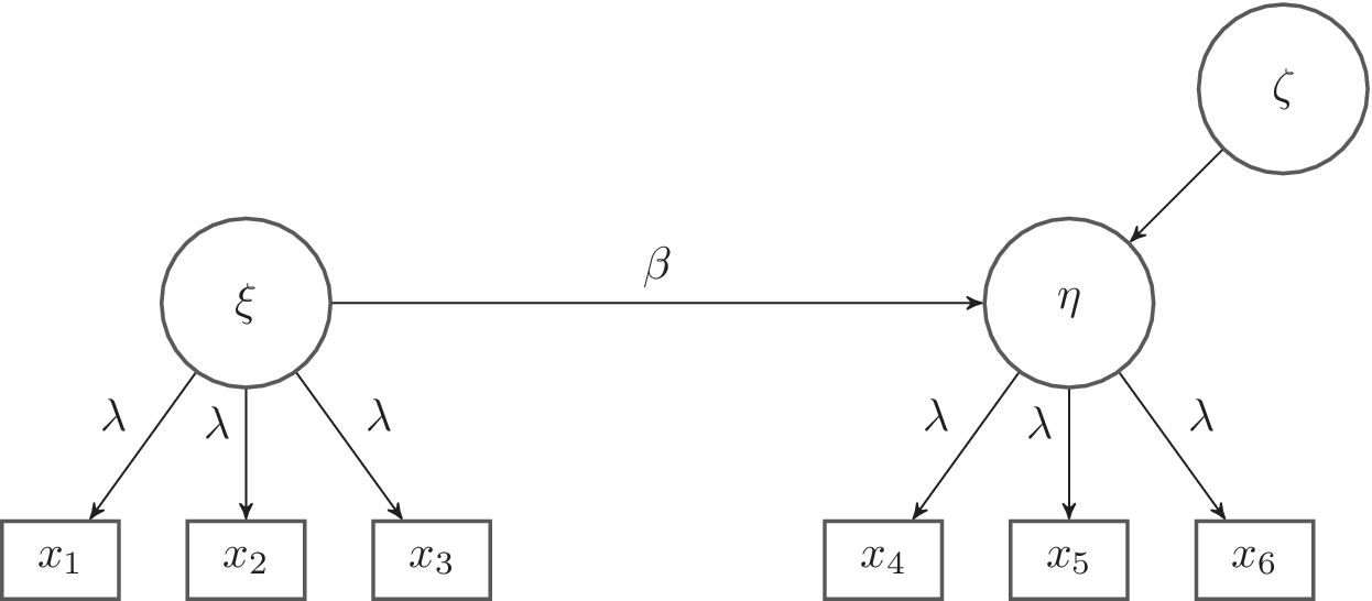
In this section, we consider a data-generating model where
$k=2$
 , with structural part given by
$ \eta = \beta \xi +\zeta $
 , where
$\xi $
 and
$\zeta $
 are univariate variables with unit variance that are uncorrelated. The measurement part of the model consists of
$p/2$
 manifest variables for each of
$\eta $
 and
$\xi $
 , so that the manifest vector
$x$
 is
$p$
 -dimensional (we only consider even
$p$
 in our illustration). The standardized factor loadings are set to a common value,
$\lambda $
 , which varies across conditions. Figure 1 depicts our model for the
$p=6$
 case.
A linear SEM. Measurement errors are not shown.

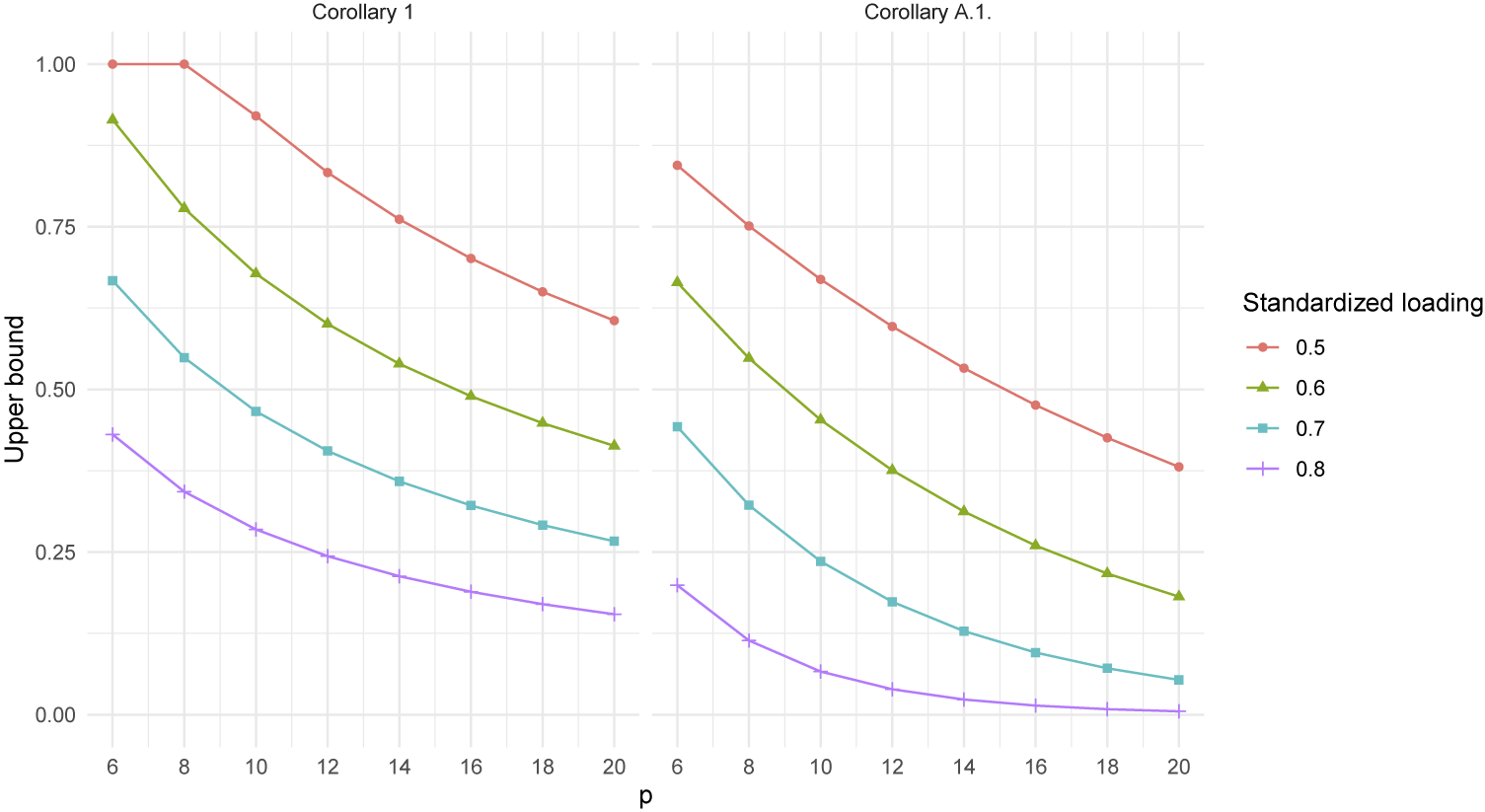
We first investigate how the bound from Corollary 1 varies with the size
$\lambda $
 of the standardized loadings and the number
$p$
 of indicators. We fixed the regression coefficient to
$\beta =1$
 . The variances of
$\eta $
 and
$\xi $
 are then 2 and 1, respectively. By setting
$\epsilon =2$
 , the bound for
$P ( |(\eta _1, \xi _1)' - (\eta _2, \xi _2)' | \geq 2 )$
 from Corollary 1 is reduced to
$\min (1,\operatorname *{\mathrm {Tr}}( \mathrm {MSE}))$
 . In Figure 2, we plot the bound across varying factor loadings and number of indicators. As expected, the bound becomes tighter when the number of indicators increases, and when the standardized loadings increase. Also, the effect of increasing factor loadings is more pronounced than increasing the number of indicators.
Upper bounds
$P ( |(\eta _1, \xi _1)' - (\eta _2, \xi _2)' | \geq 2 )$
 for varying standardized loadings and
$p$
 , the total number of indicators, with and without assuming that
$(f,u)$
 is normal.

Figure 2 Long description
A multi-panel line graph with two side-by-side panels labeled Corollary 1 on the left and Corollary 2 on the right. Both panels share a common y-axis labeled Upper bound ranging from 0.00 to 1.00 and a common x-axis labeled p ranging from 6 to 20.
In both panels, four data series represent standardized loadings of 0.5 (red circles), 0.6 (green triangles), 0.7 (blue squares), and 0.8 (purple crosses). All curves show a non-linear decrease as p increases.
Corollary 1 (Left Panel):
- The 0.5 loading starts at 1.00 for p equals 6 and 8, then curves down to approximately 0.60 at p equals 20.
- The 0.6 loading starts at 0.92 and curves down to 0.42.
- The 0.7 loading starts at 0.67 and curves down to 0.27.
- The 0.8 loading starts at 0.43 and curves down to 0.15.
Corollary 2 (Right Panel):
- All curves are shifted lower compared to Corollary 1.
- The 0.5 loading starts at 0.85 and curves down to 0.38.
- The 0.6 loading starts at 0.67 and curves down to 0.18.
- The 0.7 loading starts at 0.44 and curves down to 0.05.
- The 0.8 loading starts at 0.20 and curves down to nearly 0.00 at p equals 20.
Additionally, the right panel in Figure 2 gives the tighter bounds from Corollary A.1 in Appendix A.2, with the same configurations as above, where
$(f,u)$
 is assumed known to be normal. We see that factor indeterminacy is significantly reduced under the additional assumption of normality of
$(f,u)$
 , and the considered probability is small for a standardized loading of
$0.8$
 when
$p \geq 12$
 .
7.1 Non-normal data from independent generators
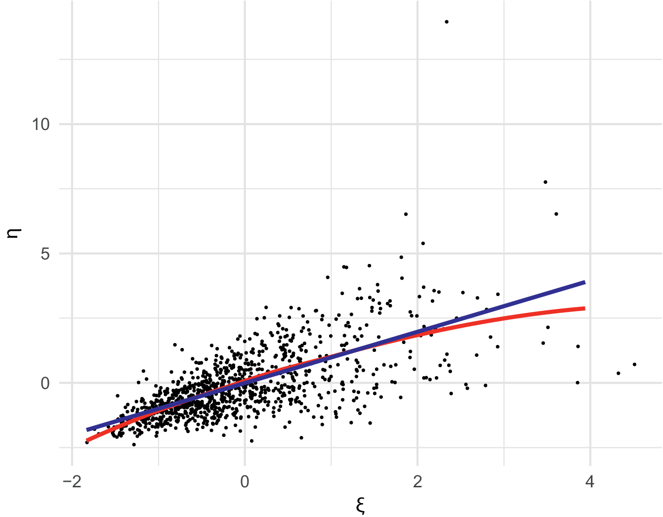
Next, we illustrate that when data are simulated via Approach 1 for a linear SEM, non-linear latent solutions are not precluded, but approximate linearity may still hold. While exact linearity is not to be expected, it is of interest to investigate whether Approach 1 creates solutions that deviate strongly from linearity. Consider the linear model in Figure 1 with
$p=6$
 ,
$\lambda =0.7$
 , and
$\beta =1$
 . The manifest variables are each specified to have skewness and kurtosis equal to 3 and 21, respectively. We generated an
$n=10^4$
 sample using the independent generator simulation method (Foldnes & Olsson, Reference Foldnes and Olsson2016) provided by the covsim (Grønneberg et al., Reference Grønneberg, Foldnes and Marcoulides2022) package, where data on the two-dimensional
$y$
 vector were simultaneously generated, also with univariate skewness and kurtosis equal to 3 and 21, respectively. The correlation between the
$x$
 and
$y$
 vectors was specified to be zero. We then generated
$\eta $
 and
$\xi $
 from
$(\eta , \xi )'=Tx+y$
 , and for an
$n=1,000$
 subsample, we plotted
$\eta $
 against
$\xi $
 in Figure 3. The figure also shows the linear regression line, as well as a loess smoothing curve calculated from the full sample with
$\xi < 4$
 . The smoothing curve follows a roughly linear trend, with only slight curvature, between
$\xi $
 and
$\eta $
 . This illustrates that using independent generator distributions for simulating manifest variables may admit factors whose association closely mimics a linear trend. Also notable is the heteroscedasticity of the
$\zeta $
 term, whose variance increases with increasing
$\xi $
 .
Scatter plot of
$\xi $
 and
$\eta $
 , generated from
$n = 1,\!000$
 observations of
$x$
 and
$y$
 drawn from the independent generator distribution. The linear regression (blue) and the loess curve (red) were calculated from an
$n=10^4$
 sample.

Figure 3 Long description
A scatter plot on a white grid background. The horizontal x-axis is labeled with the Greek letter xi and ranges from negative 2 to 4. The vertical y-axis is labeled with the Greek letter eta and ranges from 0 to 10.
* Data Distribution: A dense cluster of black data points is concentrated between xi values of negative 2 and 1, and eta values of negative 2 and 3. As xi increases beyond 1, the data points become more sparse and spread vertically, with one outlier reaching an eta value near 14 at xi approximately 2.3.
* Regression Lines: Two trend lines originate from the bottom-left. A blue linear regression line shows a constant positive slope, extending from approximately (negative 1.8, negative 1.8) to (4, 4). A red loess curve follows a similar path but exhibits a slight downward curvature as xi increases, ending at a lower eta value than the blue line at the right edge of the plot.
7.2 Normal data
Here, we show that even when
$x$
 is exactly normal, admissible factors may be highly non-linearly related. We consider the
$p=6$
 case with
$\lambda =0.3$
 and
$\beta =0.2$
 , where the manifest vector
$x$
 is specified to be multivariate normally distributed. Independently of
$x$
 ,
$y$
 was drawn from a two-dimensional discrete distribution whose covariance matrix is given by eq. (5). The
$y$
 vector has three values with nonzero probability. The resulting
$(f,u)$
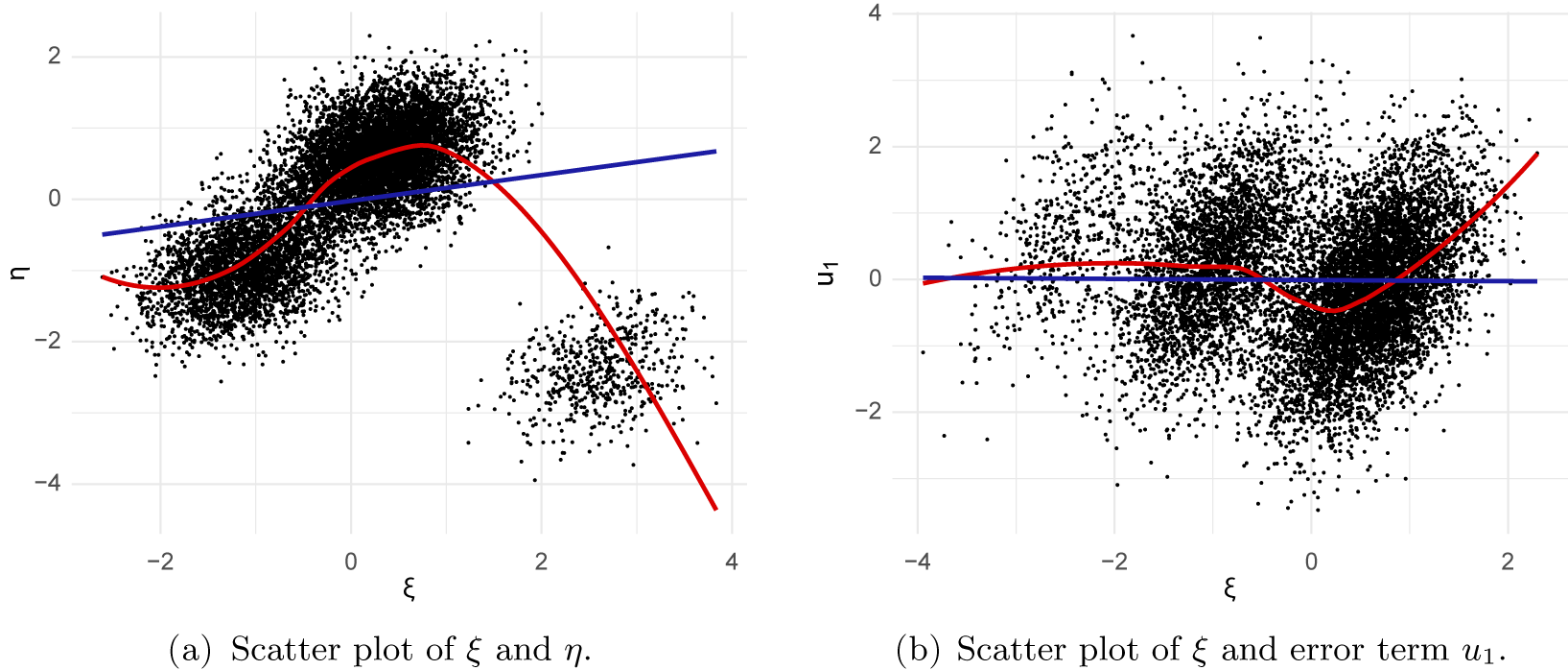
 -pair is continuous, and a scatter plot between
$\xi $
 and
$\eta $
 is presented in Figure 4a. The trend between
$\xi $
 and
$\eta $
 is far from linear, and we can discern three groups in the data. Hence, perfectly normal data may be generated from
$\xi $
 and
$\eta $
 variables that perfectly satisfy the linear SEM covariance restrictions, but whose associations are far from linear and even have group structure. This illustrates that a distinct, but hidden group structure may go undetected when fitting a linear SEM, even with multivariate normal data. In Figure 4b, we plotted
$\xi $
 realizations against realizations of the first residual error term
$u_1$
 . The pattern shows strong dependence between the two terms.
Scatter plots resulting from drawing
$n=10^4$
 observations from the multivariate normal distribution (
$\!\! x$
 ) and a discrete distribution (
$y$
 ). The linear regression (blue) and the loess curve (red) are also shown.

Figure 4 Long description
A two-panel figure with panels labeled a and b.
Panel a is a scatter plot of xi on the x-axis ranging from minus 2 to 4 and eta on the y-axis ranging from minus 4 to 2. The data points form three distinct clusters. One cluster is centered near xi equals minus 1 and eta equals minus 1. A second, larger cluster is centered near xi equals 0.5 and eta equals 0.5. A third, smaller cluster is located at xi equals 3 and eta equals minus 3. A blue linear regression line shows a slight positive slope across the entire range. A red loess curve follows the clusters, rising from left to right through the first two clusters and then dropping sharply toward the third cluster.
Panel b is a scatter plot of xi on the x-axis ranging from minus 4 to 2 and error term u sub 1 on the y-axis ranging from minus 2 to 4. The data is densely packed around the horizontal axis. A blue linear regression line is almost perfectly horizontal at u sub 1 equals 0. A red loess curve oscillates slightly around the zero line, showing a small peak near xi equals minus 1 and a small trough near xi equals 0.5 before rising at the right edge.
8 Conclusion
Factor indeterminacy is a classic issue in latent variable modeling that has received comparatively little attention in recent years. This article investigates its ramifications across three contexts where its implications are rarely explicitly addressed.
In a simulation context, factor indeterminacy guarantees that Approach 1, simulating the observed vector
$x$
 directly, is always valid in the sense that latent variables that generate
$x$
 through the model equations always exist. Intriguingly, the class of such latent variables is infinite. This means that when we simulate from a given distribution for
$x$
 , we simultaneously simulate from an infinite set of latent variable distributions, all generating the same manifest
$x$
 . For CFA simulation studies, we recommend simulating
$x$
 directly, allowing more control of features of
$x,$
 such as skewness and kurtosis compared to Approach 2, where we first simulate from latent variable distributions and generate datasets on
$x$
 through model equations. However, an important advantage of Approach 2 is that it guarantees the existence of latent variables that fulfill desired properties, such as linearity in the context of linear SEM. For simulation studies focused on SEM, we therefore recommend Approach 2 over Approach 1.
The second context is linear SEM, where we demonstrate that factor indeterminacy implies the existence of admissible latent factors with exogenous and endogenous components that are far from linearly associated. These factors exactly fulfill the modeling equations and covariance assumptions. Hence, the linearity assumption must rest on substantive domain knowledge rather than being detectable from data alone.
The third context is factor indeterminacy under additional constraints as investigated in Appendix A. We consider the case where
$f$
 and
$u$
 are known to be independent and show that unless we additionally know that
$(f,u)$
 is normal, we currently do not have a computationally feasible description of the space of admissible
$(f,u)$
 -pairs that fulfill the additional constraints. Under normality, we derive a bound for the exceedance probability of the distance between two factor solutions and see in Figure 2 that this bound is considerably smaller than what is possible under moment assumptions alone.
We next point out some directions for further research. Under assumptions securing parameter identifiability, Assumption 1 is empirically testable without substantive knowledge because it rests solely on the model structure and the parameters extracted from the covariance matrix. It leads to factor indeterminacy quantified by the bound in Corollary 1, which as illustrated in Figure 2 can lead to high probability bounds for practically relevant values of
$\epsilon $
 . Stronger assumptions reduce factor indeterminacy, and investigating what types of purely empirical (i.e., not requiring substantive knowledge) assumptions lead to a substantial reduction in factor indeterminacy is therefore important, as substantive knowledge may be faulty or missing.
We assumed throughout that the covariance model was correctly specified (Assumption 1). Factor indeterminacy under model misspecification is an interesting extension. A related issue is that Assumption 1 is mainly intended for continuous data. While continuous data methods are in some cases approximately valid for ordinal factor models (e.g., Foldnes & Grønneberg, Reference Foldnes and Grønneberg2022a), correlation is usually not a good dependency measure, and Assumption 1 together with standard additional assumptions such as
$f$
 and
$u$
 being independent is not fully compatible with ordinal data (e.g., Grønneberg and Irmer, Reference Grønneberg and Irmer2024, Appendix G, show that if
$f$
 is continuous and
$x$
 has ordinal coordinates, then
$f$
 and
$u$
 cannot be independent). Therefore, factor indeterminacy should also be considered for ordinal models, such as threshold models or IRT models.
Supplementary material
The supplementary material for this article can be found at https://doi.org/10.1017/psy.2026.10139.
Data availability statement
No empirical data were used in thisstudy. All datasets analyzed were generated through simulation andcan be reproduced using the code at https://osf.io/2jgvb/overview?view_only=b0dafeb5f31b438ab30f6ee38d7cfa67
Acknowledgements
The authors thank the Associate Editor for valuable suggestions that improved the readability of the manuscript.
Funding statement
This research received no specific grant from any funding agency, commercial, or not-for-profit sectors.
Competing interests
The authors report that there are no competing interests to declare.
Declaration of use of AI tools
In the preparation of this manuscript, the authors used ChatGPT (GPT-5.2, OpenAI) in the writing process and for generating preliminary code for the numerical illustrations. The code was edited and quality checked by the authors. We take full responsibility for the final integrity, accuracy, and content of the published work.
Appendix A. Factor indeterminacy under additional constraints
In this technical appendix, we investigate the factor indeterminacy problem under additional constraints. To our knowledge, the impact of such constraints has not been systematically studied in the existing literature.
A.1 Identification and factor indeterminacy
We start with a general discussion on the interrelation between factor indeterminacy and the assumption that
$f$
 and
$u$
 are independent.
Assumption A.1. Assume that
-
(1) $f$
and
$u$
are independent, and -
(2) (i) the factor model has no cross-loadings and each factor has at least three indicators with nonzero loadings, (ii) the coordinates of $u$
are independent, and (iii) the characteristic function of
$x$
does not vanish at any point.


Lemma 1 in Kelava et al. (Reference Kelava, Kohler, Krzyżak and Schaffland2017) shows that Assumptions 1 and A.1 lead to restrictions of the characteristic function of
$x$
 that can be inverted to uniquely find the distribution of
$(f,u)$
 . Since not all characteristic functions fulfill these restrictions, Assumption A.1 has testable implications.
Yet, in cases where the distribution of
$x$
 is compatible with Assumptions 1 and A.1(1), Proposition 1 still applies, as it assumes only Assumption 1. Therefore, there are infinitely many other admissible
$(f,u)$
 -pairs which are not compatible with Assumption A.1(1). While Assumption 1 can be tested via standard goodness-of-fit tests for covariance-based factor models, Assumption A.1(1) is only partly testable, so that even when
$x$
 has a distribution compatible with Assumption A.1(1), it need not hold. To our knowledge, this is a new observation, and it has consequences for factor analytical techniques which assume that
$f$
 and
$u$
 are independent. Assumption A.1(1) is assumed, for example, when investigating the asymptotic robustness of the normal theory maximum likelihood estimator (see, e.g., Satorra & Bentler, Reference Satorra and Bentler1990, Theorem 3.1), or when considering non-parametric trend estimation in non-linear SEM (Grønneberg & Irmer, Reference Grønneberg and Irmer2024, Assumption 2). Interestingly, the conclusions of the robustness results in, for example, Satorra and Bentler (Reference Satorra and Bentler1990) are unaffected by this distinction, because their results concern only statistical features based solely on manifest variables, and the conclusions in, for example, Satorra and Bentler (Reference Satorra and Bentler1990) therefore also hold when the manifest distribution is compatible with being generated by an independent
$(f,u)$
 -pair. In contrast, the results of both Kelava et al. (Reference Kelava, Kohler, Krzyżak and Schaffland2017) and Grønneberg and Irmer (Reference Grønneberg and Irmer2024) concern properties of
$(f,u)$
 derived under the assumption of their independence, and therefore concern only this particular pair—in addition to assuming that
$x$
 has a distribution supporting such a pair.
An example which shows that the independence between
$f$
 and
$u$
 cannot be established even when
$x$
 has a distribution that is compatible with this assumption is given in Section 7.2. There,
$x$
 is exactly normal, and there exists an exactly normal admissible
$(f,u)$
 -pair which fulfills Assumption A.1(1). The distribution of this pair is what is identified by Lemma 1 of Kelava et al. (Reference Kelava, Kohler, Krzyżak and Schaffland2017). Yet the distribution shown in Figure 4a also generates
$x$
 and produces
$x$
 observations that are numerically and distributionally indistinguishable from those produced by a normal admissible
$(f,u)$
 -pair. The strong dependence between
$f$
 and
$u$
 implied by the distribution in Figure 4a is visualized in Figure 4b.
Faced with data compatible with Assumptions 1 and A.1, and where Assumption A.1(1) is additionally known to hold through substantive means, we must reconsider the conclusions of Section 4, since the distribution of
$(f,u)$
 is identified from the distribution of
$x$
 . Therefore, for example, it is possible to test the linearity of an SEM exactly. Yet simulation work in Grønneberg and Irmer (Reference Grønneberg and Irmer2024) using the estimator suggested in Kelava et al. (Reference Kelava, Kohler, Krzyżak and Schaffland2017) indicates that unless the sample size of a dataset is extremely large, non-parametric approximations of the SEM trends may be imprecise, especially in higher dimensions.
A.2 Some results on factor indeterminacy under additional restrictions
Suppose that in addition to Assumption 1, the distribution of
$(f,u)$
 is assumed to belong to a class
$\mathcal {G}$
 . As considered above,
$\mathcal {G}$
 may be all distributions fulfilling Assumption 1 where
$f$
 and
$u$
 are independent. Let us say that a random vector
$(f,u)$
 is
$\mathcal {G}$
 -admissible for
$x$
 if
$(f,u)$
 is admissible for
$x$
 and has a distribution in
$\mathcal {G}$
 . Similarly, let us say that a Thurstone residual
$y$
 is a
$\mathcal {G}$
 -Thurstone residual if
$(f,u)$
 from eq. (6) is
$\mathcal {G}$
 -admissible for
$x$
 .
Constructing even a single
$\mathcal {G}$
 -Thurstone residual may be difficult, as we need to check whether the resulting
$(f,u)$
 -vector has a distribution contained in
$\mathcal {G}$
 . In contrast, a (standard) Thurstone residual
$y$
 is simple to produce, as it requires only that
$y$
 has zero mean and the required covariance matrix, and is uncorrelated with
$x$
 .
Let us now study the case where
$f$
 and
$u$
 are assumed to be independent. We will show that, under additional assumptions, we may generate
$y$
 independently from
$x$
 only in the fully normal case. In the non-normal case, we therefore expect that identifying
$\mathcal {G}$
 -Thurstone residuals will be difficult.
Consider
$\mathcal {G}_I$
 where
$f$
 and
$u$
 are independent, and
$u$
 has linear structure, where we recall (see Goel & DeGroot, Reference Goel and DeGroot1980, Definition 1, and the references therein) that a random vector
$z$
 has linear structure if
$z = d_0 + Dw$
 for some deterministic
$d_0,D$
 and a random vector
$w$
 with independent, nondegenerate components. Assuming that
$u$
 has linear structure is a strong assumption, which we make for mathematical feasibility, in order to apply Theorem 1 in Goel and DeGroot (Reference Goel and DeGroot1980), which refines results from Kagan et al. (Reference Kagan, Linnik and Rao1973).
Proposition A.1. Suppose Assumption 1 holds and that
$y$
 is a
$\mathcal {G}_I$
 -Thurstone residual. Define
$(f,u)$
 by (6). Assume additionally that
-
(a) $p>k$
, and each column of
$\Lambda $
has at least two nonzero entries; -
(b) if $k=1$
, then
$p\ge 3$
.


Then
$x$
 and
$y$
 are independent if and only if
$(f,u)$
 is jointly multivariate normal.
Inspired by Proposition A.1, let us therefore further study the case where
$x$
 is normal, and consider the class
$\mathcal {G}_N$
 , where
$(f,u)$
 is restricted to be normal. Since
$(x,y)$
 is an invertible linear transformation of
$(f,u)$
 , the assumption that
$(f,u)$
 is normal is equivalent to
$(x,y)$
 being normal, and since
$x$
 and
$y$
 are uncorrelated, generating all
$\mathcal {G}_N$
 -Thurstone residuals is a matter of simulating
$y \sim N(0, \mathrm {MSE})$
 independently of
$x$
 .
Under the assumption that
$(f,u)$
 is normal, we can improve the bound on factor indeterminacy given in Corollary 1.
Corollary A.1. Suppose Assumption 1 holds and that
$x$
 is normal. For any
$\epsilon>0$
 and any two
$\mathcal {G}_N$
 -Thurstone residuals
$y_1,y_2$
 inducing factor solutions
$f_1=Tx+y_1$
 and
$f_2=Tx+y_2$
 , we have

where

$Z_1,\dots ,Z_k$
 are independent
$N(0,1)$
 variables, and
$\alpha _1\ge \cdots \ge \alpha _k>0$
 are the eigenvalues of the
$\mathrm {MSE}$
 matrix.
The distribution
$F_\alpha $
 may be evaluated using algorithms from Imhof (Reference Imhof1961), and the supremum in eq. (A.1) can be computed via a numerical optimizer. The inequality (A.1) need not be sharp, but is generally an improvement over the bound in Corollary 1, as illustrated in Figure 2. It remains an open problem to identify a sharp and computationally feasible bound.
A.3 Conditional distributions and factor indeterminacy
There is a close relationship between factor indeterminacy and the conditional distribution of
$f$
 given
$x$
 . Without factor indeterminacy,
$f$
 would be solvable from
$x$
 , and
$f|x$
 would simply be a point-mass at
$f$
 as
$f$
 would be
$x$
 -measurable. Since
$f|x$
 provides a probabilistic description of what can be said about
$f$
 given knowledge of
$x$
 , it seems reasonable that this description will coincide with the descriptions considered in the present article. In this section, we show that this is so, though care must be taken, as the distribution of
$(f,x)$
 is not identified without restrictions on the distribution of
$(f,u)$
 .
The relationship between conditional distributions and factor indeterminacy seems understudied in the literature, with the exception of the normal case whose structure is very well-known, and which we take as a starting point. Suppose
$(f,u)$
 is normal. From eq. (2),
$(x,f)$
 is also normal, and under Assumption 1, the full distribution of
$(x,f)$
 is therefore fixed. Therefore, the conditional distribution of
$f|x$
 is identified from the distribution of
$x$
 .
Suppose that we independently draw at random from the resulting distribution of
$f|x$
 , resulting in, say,
$f^\circ $
 , which, through defining
$u^\circ = x - \Lambda f^\circ $
 produces a pair
$(f^\circ , u^\circ )$
 . As expected,
$(f^\circ , u^\circ )$
 is
$\mathcal {G}_N$
 -admissible for
$x$
 , see Section 3 of the Supplementary Material. Additionally, generating
$\mathcal G_N$
 -Thurstone residuals
$y$
 and forming
$f=Tx+y$
 is equivalent to sampling from the conditional law of
$\ f\mid x$
 as shown in Section 3 of the Supplementary Material. The two ways of generating admissible latent variables are therefore equivalent.
Let us now drop the normality assumption, only retaining Assumption 1. In contrast to the normal case, the joint law of
$(f,u)$
 is not fixed by the law of
$x$
 , since Assumption 1 imposes only moment restrictions. While the previous Gaussian identification argument for
$f\mid x$
 does not hold in general, a similar though more complex correspondence between conditional distributions and Thurstone residuals does hold, see Section 3 of the Supplementary Material. The operationalization of this correspondence rests on being able to produce a distribution of an admissible
$(f,u)$
 -pair, which might be computationally difficult. When
$(f,u)$
 has a distribution (non-parametrically) identified from that of
$x$
 , such as under Assumptions 1 and A.1 (using Lemma 1 in Kelava et al., Reference Kelava, Kohler, Krzyżak and Schaffland2017), the unique distribution of
$(f,u)$
 produces the starting point of the correspondence. While computing the required distribution of
$\ f|x$
 is computationally difficult, sampling independently from this distribution would be equivalent to sampling from the space of all admissible factors that are compatible with the identified distribution.
A.4 Factor indeterminacy and linear SEM as a causal model
Structural equation models are often given causal interpretations (e.g., Bollen, Reference Bollen1989, Chapters 3 and 4). In the literature on causal models, independence assumptions are foundational for providing parameters with a causal interpretation. We here consider these independence assumptions in light of the theory developed above.
For simplicity, suppose
$k=2$
 , that Assumption 1 holds, and that
$f = (\eta , \xi )'$
 is assumed to have standardized marginals. A linear structural model with a causal interpretation is then

Here, for
$\beta _1$
 to be seen as a causal parameter, the independence between
$\xi $
 and
$\zeta $
 is crucial (see, e.g., Pearl, Reference Pearl1995, Section 2.2, and the earlier works cited therein).
Suppose we fit the structural model in eq. (A.2) to a sample drawn from
$x$
 . Interpreting the resulting parameter estimate of
$\beta _1$
 in a causal manner requires that eq. (A.2) holds. In general, this requires two things. First, the distribution of
$f$
 must be compatible with being generated as in eq. (A.2). Second, we must argue that any alternative structural model that is compatible with the distribution of
$f$
 is incorrect. The existence of such alternative models is well-known in the causal literature (e.g., Pearl, Reference Pearl2009, Section 1.2) and in classical SEM (e.g., Bollen, Reference Bollen1989, Chapter 3, pp. 67–79).
The difficulty of these steps is exacerbated by not being able to observe
$f$
 realizations directly. A first complication comes from factor indeterminacy. To test whether the distribution of
$f$
 is compatible with eq. (A.2), the practitioner will need assumptions in addition to Assumption 1. Suppose the distribution of
$x$
 is such that, under these additional assumptions,
$f$
 is indeed compatible with eq. (A.2). Even then, the additional assumptions made to test eq. (A.2) are only partly testable, as Proposition 1 implies that there is a large space of admissible
$(f,u)$
 pairs where
$f$
 is incompatible with eq. (A.2). Therefore, the additional assumptions needed to defend eq. (A.2) must be substantive. A second complication comes from constructing a test for the testable implications of the independence statement in eq. (A.2) based on observations from
$x$
 . Currently, no such generally applicable test exists.
These methodological and substantive issues complicate a causal interpretation of linear SEM estimates. Our illustration in Section 7.2 considers the best-case scenario of multivariate normality for linear SEM. Here, Assumption 1 and Assumption A.1(2)(i) and (iii) hold, and
$x$
 is compatible with Assumption A.1(1) and Assumption A.1(2)(ii). Under Assumption A.1(1),
$(f,u)$
 is multivariate normal (e.g., Muirhead, Reference Muirhead1982, Theorem 1.2.13), and eq. (A.2) holds for the standard regression representation of
$\eta $
 and
$\xi $
 . Yet many other admissible pairs exist, and the illustration in Section 7.2 shows, first, that
$(f,u)$
 need not be normal and, second, that the induced pair
$(\eta ,\xi )'$
 need not fulfill eq. (A.2) even as a rough approximation.
A.5 Factor indeterminacy and simulation studies
We now revisit the simulation discussion from Section 3 in light of the preceding analysis of factor indeterminacy under restrictions. Our main finding was that factor indeterminacy ensures the validity of Approach 1, as a large class of admissible factors always exists. Furthermore, Approach 2 can be viewed as an instance of Approach 1, offering the advantage of guaranteeing the existence of an admissible
$(f,u)$
 -pair with controlled properties, such as linearity in linear SEM.
Factor indeterminacy does not further influence the interpretation of simulation results, as long as the statistical technique under scrutiny is evaluated using only manifest variables as input. However, in some studies, a statistic derived from manifest variables is compared to factors, such as when testing the performance of empirical factor scores as estimators of the factor
$f$
 that generated the data (e.g., Acito & Anderson, Reference Acito and Anderson1986; Bauer et al., Reference Bauer, Baldasaro and Gottfredson2012; Curran et al., Reference Curran, Cole, Bauer, Hussong and Gottfredson2016; Grice, Reference Grice2001; Grice & Harris, Reference Grice and Harris1998; Grønneberg & Irmer, Reference Grønneberg and Irmer2024; Kelava et al., Reference Kelava, Kohler, Krzyżak and Schaffland2017). In such studies, factor indeterminacy should be taken into account. In the following, we limit our discussion to simulation studies that compare factor scores to factors. To our knowledge, such factor-score simulation studies have all employed Approach 2, since it is not immediately clear how Approach 1 might be set up for such a simulation study. We therefore start by investigating factor-score simulations under Approach 1. We suppose that Assumption 1 holds.
From Proposition 1(i), we may simulate
$(x,y)$
 where
$y$
 is a Thurstone residual and compute
$(f,u)$
 via eq. (6). The resulting distribution of
$f$
 depends crucially on which Thurstone residual is chosen, and the resulting factor distribution may be sensitive to the distribution of
$y$
 . A simple illustration of this is given in Section 7.2, where
$x$
 is normal. When
$y$
 is independent of
$x$
 and normal, the resulting
$(f,u)$
 is the familiar normal factor solution. In contrast, the Thurstone residual we draw from in Section 7.2 produces a factor solution
$(f,u)$
 where the components of
$f$
 are highly non-linearly related, and numerically very different from the expected normal solution (see Figure 4a).
It is clear that factor-score performance statistics would be very different for the two induced factors, and that defending appropriate choices of Thurstone residual distributions may be difficult without further restrictions on the admissible factors, such as assuming that the distribution of
$(f,u)$
 is contained in an appropriate class
$\mathcal {G}$
 . As seen from Proposition A.1, constructing
$\mathcal {G}$
 -Thurstone residuals is in most cases difficult outside simple cases such as normality.
From this, Approach 1 may seem unsuitable for factor-score simulations. However, practically relevant data distributions are more easily approximated using Approach 1 than using Approach 2, and realistic manifest distributions may even be incompatible with the theoretical restrictions often made on the distribution of
$(f,u)$
 when employing Approach 2. Producing a class of Thurstone residuals
$y$
 with a fixed distribution and studying how a factor score compares to the induced
$f$
 is representative of a single member out of an infinite class. As long as this non-uniqueness is understood, the resulting study could in theory be more realistic than factor-score simulations using Approach 2, which usually consider highly stylized distributions where, for example,
$f$
 and
$u$
 are independent.
Consider now Approach 2, where we, for concreteness, assume that we generate normal
$(f,u)$
 following the moment restrictions of the model considered in Section 7.2, and then generate
$x$
 via eq. (2). While, to our knowledge, all simulation studies for factor-score simulation have compared factor scores to the
$(f,u)$
 -pair used in the simulation, any admissible
$(f,u)$
 -pair generates the numerically identical
$x$
 , and the highly non-normal factor solution
$f$
 considered in Section 7.2 is on the same footing as the normal solution. To justify comparing the actual
$(f,u)$
 -pair used for generating
$x$
 with the factor score, we must add context to the simulation study, arguing that we emulate a realistic condition based on a researcher’s substantive knowledge that allows us to single out the generated
$(f,u)$
 -pair or its distribution. For example, Assumption A.1 may be justified by substantive knowledge. In the case of a normal
$x$
 , this would imply that
$(f,u)$
 is normal, and the mixture distribution of Section 7.2 could be ruled out.
Even when the distribution of
$(f,u)$
 is identified from
$x$
 and
$(f,u)$
 is normal, the numerical values of the factors are indeterminate (see Section A.2). Statistics used in factor-score simulations depend only on the distribution of
$(x, \ f)$
 . Under the assumption that the distribution of
$(f,u)$
 is identified by the distribution of
$x$
 , also the distribution of
$(x, \ f)$
 is identified, because
$x = \Lambda f + u$
 . The distribution of
$(x,f)$
 can be drawn, for example, by using the latent variables produced during the equation-by-equation simulation step, thereby justifying current simulation practice using Approach 2, as long as the identification of the distribution of
$(f,u)$
 is assumed given.
Let us consider an illustration of this argument where
$(f,u)$
 is assumed to be normal. Suppose we generate
$R$
 datasets each of sample size
$n$
 . For each dataset
$r=1,2, \ldots , R$
 , we compute a factor-score estimator
$\hat f_{r,n}$
 and compare that with the realized factor
$f_r$
 we used in the simulation through a statistic of the form

using some distance function, for example, the Euclidean distance
$D(x,y) = |x-y|$
 . Letting
$o_P(1)$
 be a quantity converging to zero in probability as
$R \to \infty $
 , the law of large numbers implies that

Here, the limiting quantity
$ \operatorname {E} D(\hat f_{1,n}, f_1)$
 depends only on the joint distribution of
$(x, \ f)$
 , which is unique. That is, we supposed we used the factors
$f_r$
 to compute
$\Delta _{n,R}$
 . Each of these factors is just one representative of the space of
$\mathcal {G}_N$
 admissible factors. And while numerically different representatives would give different values for
$\Delta _{n,R}$
 for finite
$R$
 , any choice among the class of
$\mathcal {G}_N$
 -admissible solutions gives the same limiting quantity.






 Open access

