2.1 Equations of motion for the turbulence fields

We combine the Eulerian description of the turbulent velocity, temperature and vapour content fields with the Lagrangian description of the ensemble of cloud water droplets. Condensation rate, liquid water content and local supersaturation determine the diffusional growth of the individual cloud water droplets. Typical cloud droplet concentrations of the order of $10^{2}~\text{cm}^{-3}$ result in approximately 10–100 million individual droplets. They are treated as inertial point particles with Stokes drag and gravitational settling. We monitor their position, their velocity and the droplet radius.

Turbulence is simulated in a Cartesian slab volume with a maximum size of $2~\text{m}\times 1~\text{m}\times 1~\text{m}$ . The Kolmogorov scale of $\unicode[STIX]{x1D702}_{K}\approx 1~\text{mm}$ is chosen here in all runs, which is typical for cumulus clouds (Lehmann, Siebert & Shaw Reference Lehmann, Siebert and Shaw2009). Recall that the Kolmogorov scale defines the smallest vortices in the turbulent cloud, the end of the turbulent inertial cascade.

The turbulent velocity field $u_{i}(x_{j},t)$ , the temperature field $T(x_{j},t)$ and the pressure field $p(x_{j},t)$ are the fields necessary for the description of dry turbulent convection. In the following, $x_{i}$ ,  $x_{j}$ or $x_{k}=(x,y,z)$ . We use the Einstein sum convention for indices $i,j,k$ . In the case of phase changes during the mixing process, we have to add two mixing ratios, the vapour mixing ratio field $q_{v}(x_{j},t)=\unicode[STIX]{x1D70C}_{v}/\unicode[STIX]{x1D70C}_{d}$ and the liquid water mixing ratio field $q_{l}(x_{j},t)=\unicode[STIX]{x1D70C}_{l}/\unicode[STIX]{x1D70C}_{d}$ , since phase changes are present. Here, $\unicode[STIX]{x1D70C}_{d}$ , $\unicode[STIX]{x1D70C}_{v}$ and $\unicode[STIX]{x1D70C}_{l}$ are mass densities of dry air and water vapour, and liquid water content, respectively. The Eulerian equations in the Boussinesq approximation are then given by

The buoyancy field $B$ in (2.2) depends on three fields, the temperature $T$ , the vapour mixing ratio $q_{v}$ and the liquid water mixing ratio $q_{l}$ , respectively. It is given by

Here, $\unicode[STIX]{x1D708}$ is the kinematic viscosity of air and $g$ is the gravitational acceleration. The quantity $\unicode[STIX]{x1D70C}_{0}$ is the reference value for dry air mass and $\unicode[STIX]{x1D700}=0.608$ . The temperature fluctuations are given by

and the vapour mixing ratio fluctuations by

with $\langle \cdot \rangle$ being a volume average. The quantity $c_{p}$ is the specific heat at constant pressure, $L$ is the latent heat, $\unicode[STIX]{x1D705}$ is the diffusivity of the temperature, and $D$ is the diffusivity of the vapour mixing ratio. Here, $\unicode[STIX]{x1D705}\approx D$ .

2.2 Lagrangian model for cloud water droplets

In our numerical approach, the liquid water mixing ratio $q_{l}$ and the condensation rate $C_{d}$ are calculated in the Lagrangian frame of reference since particles are advected in the turbulent flow. Their properties have to be ‘translated’ into the Eulerian frame of reference for use in (2.3) and (2.4). In turn, flow field properties have to be determined at the droplet position in order to advance the Lagrangian equations as visible in (2.8)–(2.11) below.

Since the Stokes numbers and the mass loading are small, the feedback of the droplets on the flow is only considered as the drag of liquid mass on the flow, which is included by the term $-gq_{l}$ in the buoyancy in (2.5). Additional terms in the equation of motion that exist even for low Reynolds number include Faxen term, added mass, pressure gradient, and Basset history forces (see Crowe, Sommerfeld & Tsuji Reference Crowe, Sommerfeld and Tsuji1998, § 4.3). For our simulation conditions, the forces are estimated to have the following orders of magnitude relative to Stokes drag: Faxen $10^{-5}$ , added mass $10^{-6}$ , pressure gradient $10^{-3}$ , Basset history $10^{-2}$ . This is consistent with the conclusion from other works that Stokes drag is the dominant contribution for heavy particles in turbulent gas flows for a density ratio of ${\sim}10^{-3}$ (Shaw Reference Shaw2003; Bergougnoux et al. Reference Bergougnoux, Bouchet, Lopez and Guazzelli2014; Olivieri et al. Reference Olivieri, Picano, Sardina, Iudicone and Brandt2014).

Figure 1.

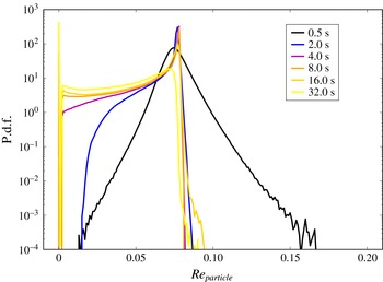
Probability density function of the particle Reynolds number for different times of the mixing process. Data are obtained from simulation run TNIa, which is displayed in table 1.

The Lagrangian evolution of each of the $N_{d}$ cloud droplets is described by the following set of equations:

Here, $X_{i}$ is the space coordinate vector at each particle position and $V_{i}$ its velocity, which differs from the velocity of the air, $u_{i}$ , at the droplet position. Gravitational acceleration is $g_{i}=-g\unicode[STIX]{x1D6FF}_{zi}$ and particle response time (or Stokes time) is $\unicode[STIX]{x1D70F}_{p}$ . The definition of $\unicode[STIX]{x1D70F}_{p}$ follows later in the text. The particle response time is adjusted to the droplet radius in the dynamical evolution. Here we use the linear Stokes drag model, since the particle Reynolds number

with droplet diameter $d$ and the absolute velocity difference $|u_{i}(X_{j},t)-V_{i}(X_{j},t)|$ , is always smaller than $0.1$ (see figure 1). According to investigations of Bergougnoux et al. (Reference Bergougnoux, Bouchet, Lopez and Guazzelli2014) nonlinear corrections can therefore be excluded for small Stokes numbers $St<0.1$ . The droplet radius growth by vapour diffusion is described by the following equation (see e.g. Kumar et al. Reference Kumar, Schumacher and Shaw2013 and references therein),

where $K$ is a constant. Equations (2.8)–(2.11) are coupled to equations (2.1)–(2.5) and are simultaneously integrated forward in time. The Lagrangian equations are still solved even for droplets that are fully evaporated. Particles with radius $r\leqslant 0.5~\unicode[STIX]{x03BC}\text{m}$ are considered to have very small inertia and are handled as passive Lagrangian tracers. Therefore the Lagrangian dynamics simplify to only (2.8) with $\text{d}X_{i}/\text{d}t=u_{i}(X_{j},t)$ excluding (2.9). Throughout the paper all Lagrangian statistics include particles with zero radius, unless otherwise noted in the text.

Table 1.

Parameters of the different direct simulation runs. We denote the run with the same turbulent kinetic energy (TKE) in- and outside the cloud as TTI for turbulent–turbulent interface, the runs with different levels as TNI for turbulent–non-turbulent interface. The second column displays the number of grid points covering the whole simulation domain, the third column the size of the rectangular box. The fourth column stands for the approximate ratio of the TKE in the clear air half ( $k_{2}$ ) and the cloudy half ( $k_{1}$ ). The Reynolds number is given by $Re=u_{rms}L_{x}/\unicode[STIX]{x1D708}$ . The Kolmogorov scale $\unicode[STIX]{x1D702}_{K}$ will match the uniform grid spacing $a$ in all cases. In the penultimate column $N_{d}$ is the total number of droplets. The total time span $t_{total}$ of the integration is given in the last column.

Table 2.

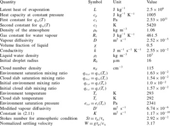
List of constants, reference values and initial simulation parameters. Particle time scale $\unicode[STIX]{x1D70F}_{p}$ and Kolmogorov time scale $\unicode[STIX]{x1D70F}_{\unicode[STIX]{x1D702}}$ are defined in table 3. The Kolmogorov velocity is defined as $v_{\unicode[STIX]{x1D702}}=(\langle \unicode[STIX]{x1D716}\rangle \unicode[STIX]{x1D708})^{1/4}$ .

Table 3.

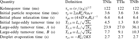
List of important time scales in the mixing process. Times $A$ and $B$ are indicated as the first two vertical dotted lines in figure 3(a,b). Quantities $k_{0}$ , $k_{A}$ , $k_{B}$ and $\langle \unicode[STIX]{x1D716}_{B}\rangle$ refer to the values of the quantities at $t=0$  s,  $t\approx 4$  s and $t\approx 15$  s for cases TNIa and TTIa. Quantities $k_{B}$ and $\langle \unicode[STIX]{x1D716}_{B}\rangle$ are taken at time $t\approx 24$  s for TNIb. In all cases $\langle \unicode[STIX]{x1D716}_{B}\rangle \approx 10~\text{cm}^{2}~\text{s}^{-3}$ , which is a typical atmospheric value. Time scale $T_{L,B}$ is chosen as a typical eddy turnover time.

The supersaturation field $S$ is determined from the vapour mixing ratio and is given by

The saturation vapour mixing ratio $q_{vs}(T)$ has to be determined from the temperature as a solution of the Clausius–Clapeyron equation. It is given by

with the specific gas constant for vapour $R_{v}$ . The saturation pressure $e_{s}$ is given by $e_{s}(T)=c_{1}\exp (-c_{2}/T)$ (see Rogers & Yau Reference Rogers and Yau1989 for more details). Here, $c_{1}$ and $c_{2}$ are constants, which are listed in table 2.

Practically, for the conditions of this study, the droplet collision rate is expected to be negligible over the time we have simulated. Initially the droplets are all of a single size, so the primary contributions to collision rate are shear and inertial effects (see e.g. Shaw Reference Shaw2003). As the distribution becomes broader, differential sedimentation becomes dominant. The time scale for a collision due to differential sedimentation scales as $\unicode[STIX]{x1D70F}_{1,2}\sim (n\unicode[STIX]{x03C0}(d_{1}+d_{2})^{2}|v_{t,1}-v_{t,2}|\unicode[STIX]{x1D716}_{1,2})^{-1}$ , where subscripts 1 and 2 represent droplets of two sizes, $n$ is droplet number density, $d$ is droplet diameter, $v_{t}$ is terminal speed, and $\unicode[STIX]{x1D716}$ is the collision efficiency (Rogers & Yau Reference Rogers and Yau1989). For typical droplet sizes and best estimates of $\unicode[STIX]{x1D716}$ , this time is of order 1–10 h, thus much greater than the large-eddy turnover time. Furthermore, turbulent enhancements of the collision rate are less than a factor of 2 for the simulated conditions (Grabowski & Wang Reference Grabowski and Wang2013).

2.3 Evaluation of condensation rate

The liquid water mixing ratio is calculated by summing up the liquid water mass of the droplets in each grid cell. To close the coupled system of Eulerian and Lagrangian equations (2.1)–(2.12), we determine the condensation rate field $C_{d}(x_{i},t)$ by

Here, $m_{a}$ is the mass of air per grid cell, $m_{l}$ is the mass of liquid per grid cell and the sum from $\unicode[STIX]{x1D6FD}=1$ to $\unicode[STIX]{x1D6E5}$ collects the droplets inside each grid cell of size $a^{3}$ surrounding the spatial point $x_{i}$ (see also Vaillancourt et al. Reference Vaillancourt, Yau and Grabowski2001). The mass of liquid $m_{l}$ is the sum over all droplets, which are spheres. Together with (2.11) for the change of the droplet radius, this results in the final expression for the condensation rate to the right. The transmission of the Eulerian field values at grid positions to the enclosed droplet position is done by trilinear interpolation. The inverse procedure is necessary for the calculation of the condensation rate, which is evaluated first at the droplet position and then redistributed to the nearest eight grid vertices.

2.4 Numerical method

The DNS applies a high-resolution pseudospectral method based on a Fourier series expansion of all Eulerian turbulence fields (Schumacher, Sreenivasan & Yakhot Reference Schumacher, Sreenivasan and Yakhot2007). Spectral methods converge exponentially fast and provide an accurate approximation of the strongly fluctuating gradients of the turbulent fields at the smallest scales. The simulation domain consists of an equally spaced mesh grid with up to $2048\times 1024\times 1024$ grid points for a box size $L_{x}\times L_{y}\times L_{z}$ of up to $2~\text{m}\times 1~\text{m}\times 1~\text{m}$ . We apply periodic boundary conditions in all three directions. A second-order time stepping with a predictor–corrector scheme is used. Our spectral resolution always satisfies $k_{max}\unicode[STIX]{x1D702}_{K}\gtrsim 3$ , such that the trilinear interpolation in the Lagrangian model is expected to be sufficient.

The simulation program is parallelized in two dimensions using the Message Passing Interface and a two-dimensional domain decomposition of the whole volume into slabs. Table 1 shows all simulation runs and lists some important parameters. Throughout the whole paper, we will name the case with equal turbulence level the turbulent–turbulent interface case (TTI), the case with a lower turbulence level in the clear air region outside the cloud the turbulent–non-turbulent case (TNI). The latter corresponds to the shearless mixing layer. Cases TTIa and TNIa will be directly compared. Run TNIb represents the shearless mixing case with a larger simulation domain, which allows us to explore the importance of the range of scales.

The production runs were conducted on up to 4096 processor cores. The most computationally expensive job TNIb took 18 days for 85 000 time steps to be completed. Jobs TNIa and TTIa were run on 512 cores and took approximately 6 days for 120 000 time steps. The particle tracking is also fully parallelized. Particle data are exchanged between processors when the droplet leaves the subdomain which is associated with a processor. For the biggest simulations, particle tracking takes approximately 15 % of the total time of an integration time step. We continue to track droplets even when they are fully evaporated, although these droplets no longer affect the dynamics.

2.5 Initial shearless mixing layer configuration

The velocity field is initialized in wavenumber space by random Fourier amplitudes with a predefined energy spectrum (Rogallo Reference Rogallo1981). This results in integral length scales of the initial configuration that are smaller than $L_{y}~(=L_{z})$ . For example, $L(t=0)\approx 11~\text{cm}$ for run TNIa. For the cases of a shearless mixing layer (TNI), the velocity field $u_{i}(x_{j})$ is transformed to physical space and rescaled by a mixing function $g(x)$ as used by Tordella & Iovieno (Reference Tordella and Iovieno2011):

with

Indices 1 and 2 correspond to $V_{1}$ and $V_{2}$ , respectively. The ratio of turbulence levels as displayed in table 1 follows from

The blending factor $c$ in the scaling function $g(x)$ determines the width of the mixing layer. We take the same value of $c=50$ such that the initial interface layer occupies $L_{x}/50$ . Incompressibility is re-established in Fourier space by projection

which satisfies $\ell _{j}\widehat{u}_{j}(\ell _{x},\ell _{y},\ell _{z})=0$ with $\ell _{x}$ , $\ell _{y}$ and $\ell _{z}$ being the wavenumbers.

The vapour mixing ratio and temperature fields, $q_{v}(x_{i},t=0)$ and $T(x_{i},t=0)$ , are rescaled with the same function as the velocity. Amplitudes are matched to values obtained in the CARRIBA experiments. Details are given in table 2. The profiles are chosen such that the contributions of temperature and vapour content compensate each other in the buoyancy $B$ in (2.5). Once all Eulerian fields are set up, we relax the velocity components in a few integration time steps. The final negative buoyancy is due to the additional liquid water content in the form of the initially monodisperse droplets which are seeded randomly in  $V_{1}$ .

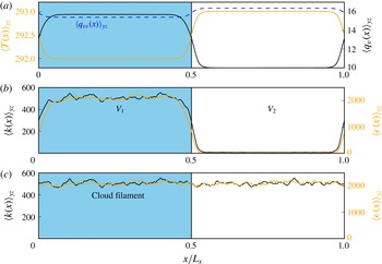
Figure 2 displays the initial configuration for cases TNI and TTI. The saturation vapour mixing ratio is marked as a dashed line in figure 2(a) corresponding to (2.13). The vapour and temperature profiles are matched to the CARRIBA measurement data with a humidity of approximately $60\,\%$ in the clear air region. The temperature jumps by 1 K across the interface. Note that we take a lower temperature in the cloud compared to the environment. As already stated in the introduction, the shearless mixing layer configuration in our study represents a typical situation at the side of a warm dissolving cumulus cloud.

Figure 2.

Initial configurations of the DNS. The slab is divided into a cloudy half-box $V_{1}$ and a clear air half-box $V_{2}$ . We display initial profiles of the two configurations discussed in the work. A case with a very low level of flow turbulence outside the cloud filament (TNI) is shown in (b) and a case with the same turbulence level (TTI) in- and outside the cloud is shown in (c). (a) Profiles of water vapour mixing ratio $q_{v}(x,t=0)$ (black/dark solid line), the temperature $T(x,t=0)$ (orange/light solid line) and saturation vapour mixing ratio $q_{vs}(x,t=0)$ (blue/dark dashed line). These profiles are the same for TNI and TTI. (b) Turbulent kinetic energy (TKE) (black/dark solid line) and kinetic energy dissipation rate (orange/light solid line) averaged in $y$ – $z$ planes at $t=0$ for TNI. (c) Same quantities as in panel (b) for the case TTI. Temperature $T$ is measured in K, vapour mixing ratio $q_{v}$ in $\text{g}~\text{kg}^{-1}$ , TKE $k$ in $\text{cm}^{2}~\text{s}^{-2}$ and kinetic energy dissipation rate $\unicode[STIX]{x1D716}$ in $\text{cm}^{2}~\text{s}^{-3}$ .

Figure 3.

Evolution of different volume averages in the course of the decaying turbulence runs: (a) mean TKE $k$ ; (b) mean kinetic energy dissipation rate $\langle \unicode[STIX]{x1D716}\rangle$ : (c) mean vapour mixing ratio $\langle q_{v}\rangle$ ; and (d) mean temperature $\langle T\rangle$ . Temperature $T_{\infty }$ is indicated as a horizontal dashed line. 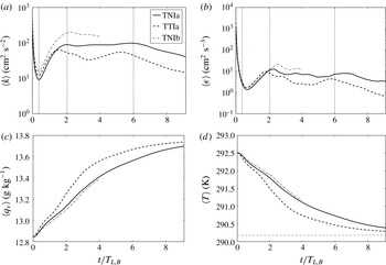Time is given in units of a large-scale eddy turnover time $T_{L,B}$ , which is listed in table 3. The approximate extension of the four evolution stages is indicated by vertical dotted lines in the upper panels.

We take the initial set-up in such a way that liquid water is completely transformed into vapour, i.e. all droplets evaporate eventually. To estimate the necessary amplitudes, we start with a set of equations that describe the mixing of two parcels as suggested by Gerber, Frick & Jensen (Reference Gerber, Frick and Jensen2008). The equations are derived from the conservation of liquid potential temperature $\unicode[STIX]{x1D703}_{l}=T-(L/c_{p})q_{l}$ and total water mass $q_{total}=q_{v}+q_{l}$ and are given by

They are based on the idea that parcels of air with liquid potential temperature and total water mixing ratio mix linearly. Therefore, the left-hand side represents the state after the mixing of the two parcels and the right-hand side represents the individual parcels, which differ by the mixing fraction $\unicode[STIX]{x1D712}$ and $1-\unicode[STIX]{x1D712}$ . Here, the initial liquid water mixing ratio inside the cloud $q_{lc}$ and the final temperature at the end of the mixing process are the unknowns. We assume that the final liquid water mixing ratio $q_{l}=0$ . The other variables are the cloud volume fraction $\unicode[STIX]{x1D712}$ , the vapour mixing ratio $q_{ve}$ and temperature $T_{e}$ in the environment $V_{2}$ . The vapour mixing ratio $q_{vc}$ and temperature $T_{c}$ are the values in the cloudy subvolume $V_{1}$ . Solving the equations with $N_{d}$ from table 1 and $R_{0}$ from table 2 results in a temperature of $T_{\infty }=290.2~\text{K}$ at the end of the mixing process.

3.1 Global volume-averaged quantities

Our simulation runs decay freely without additional body forces that enforce a statistically stationary regime. The feedback by the buoyancy is the only term that can amplify the fluid motion transiently. Therefore, the mixing as a whole is a transient process that cannot be characterized by a single set of characteristic time scales as statistically stationary turbulence. We are interested in the time evolution of the turbulent kinetic energy (TKE), $k$ , and the mean squares of the temperature, $k_{T}$ , and the vapour fluctuations, $k_{q}$ , respectively, given by

The TKE profile is depicted in figure 3. We also display the mean of the kinetic energy dissipation rate field,

as well as the means $\langle q_{v}(t)\rangle$ and $\langle T(t)\rangle$ . The brackets $\langle \cdot \rangle$ denote again spatial averaging over the whole simulation domain $V=V_{1}\cup V_{2}$ (see figure 2).

In order to obtain the balance equations for quantities (3.1a–c ), we multiply the three momentum balance equations with the corresponding $u_{i}$ , which implies automatically the Einstein’s summation rule, the temperature fluctuation equation with $T^{\prime }$ and the one for the water vapour mixing ratio fluctuations with $q_{v}^{\prime }$ , respectively. After taking the volume average, applying Gauss’s theorem and using the fact that flux terms across the boundary disappear in the case of periodic sidewalls, we arrive at the evolution equations, which are given by

Quantities $\langle \unicode[STIX]{x1D716}_{q}(t)\rangle =D\langle |\unicode[STIX]{x1D6FB}q_{v}^{\prime }|^{2}\rangle$ and $\langle \unicode[STIX]{x1D716}_{T}(t)\rangle =\unicode[STIX]{x1D705}\langle |\unicode[STIX]{x1D6FB}T^{\prime }|^{2}\rangle$ are the dissipation rate of vapour variance and the thermal dissipation rate, respectively. We will focus on describing the TKE balance (3.3) in the following because the other two quantities, $k_{q}$ and $k_{T}$ , decay steadily for most of the time during the mixing process.

The buoyancy feeds back to the flow in three different ways – namely via temperature, vapour and liquid water contents – and thus contributes to the TKE production via the buoyancy flux term in (3.3). Droplets that enter the subsaturated region will shrink and thus cause a local evaporative cooling. This will lower the magnitude of the adjacent temperature field and, together with the additional drag due to gravitational settling of the droplets, results in a negative local buoyancy contribution ( $B<0$ ). A downdraught eventually forms due to gravitational acceleration ( $u_{z}<0$ ) such that the product of the two quantities turns into a local gain term ( $u_{z}B>0$ ) for the TKE. A local loss will be caused by an updraught $u_{z}>0$ and $B<0$ . The kinetic energy dissipation rate is a positive definite quantity and thus always a sink of TKE.

Following from figure 3 for the TKE, the mixing process can be divided into four different stages:

1. (i) The first stage lasts the first half eddy turnover time and is characterized by a very rapid decay of turbulence. The small eddies are dissipated quickly until the first droplets start to evaporate and consume heat in their vicinity. The end of this period is marked by a dotted line in figure 3(a,b).

2. (ii) The second stage displays a recovery of TKE due to the combined action of velocity downdraught and negative buoyancy. Consequently, kinetic energy dissipation also increases. Both $k$ and $\langle \unicode[STIX]{x1D716}\rangle$ reach a local maximum after up to two eddy turnover times indicated by a second dotted line in figure 3(a,b). The large-scale eddy turnover time at the end of this period $T_{L,B}$ (see table 3) is chosen as the reference time for further comparison.

3. (iii) The third stage starts when production and dissipation of kinetic energy are of nearly the same size. The mixing process now passes through a phase that is close to statistical stationarity, at least in terms of the TKE. This period lasts approximately four eddy turnover times in configurations TNIa and TTIa. It is expected to take longer in the larger domain of run TNIb, but computational resources limited the time that could be followed for that case. Significant buoyancy production is achieved on the one hand when a large portion of cloudy air with droplets entrains the clear air region, which is the case during this stage of evolution. The time this takes is given by the large-eddy turnover time $T_{L}$ . In order to cause colder downdraughts, on the other hand, droplets have to evaporate. This time interval is quantified by the phase relaxation time $\unicode[STIX]{x1D70F}_{ph}$ and the single droplet evaporation time $\unicode[STIX]{x1D70F}_{ev}$ , depending on their relative magnitudes (Lehmann et al. Reference Lehmann, Siebert and Shaw2009). Definitions and typical values for these time scales are given in table 3. For this stage $\langle \unicode[STIX]{x1D716}\rangle \approx 10~\text{cm}^{2}~\text{s}^{-3}$ in all cases, which results in $\unicode[STIX]{x1D702}_{K}\approx 1.35~\text{mm}$ and $R_{\unicode[STIX]{x1D706}}=187$ , 133 and 419 for TNIa, TTIa and TNIb, respectively.

4. (iv) The fourth and final stage starts after approximately six eddy turnover times and marks the eventual decay of all quantities and the finalization of the mixing process in our system. The mean temperature approaches the estimate that we obtained from (2.19) and (2.20). This value of $T_{\infty }=290.2$  K is indicated by a dashed line in figure 3(d). The total temperature variation remains small in the course of the evolution. As seen in figure 3(d), there is a total drop by $\unicode[STIX]{x0394}T=2.5$  K. For these variations, we can keep all material parameters as constants (see also Zonta & Soldati (Reference Zonta and Soldati2014) for a study of temperature-dependent effects).

To all panels of figure 3, we add the data from the run in the largest domain, TNIb. A larger TKE for TNIb is in line with a larger domain and larger Reynolds number. Note also that the eddy turnover time, $T_{L}$ , becomes larger compared to TNIa (see table 3).

Figure 4.

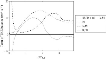
Time evolution of the three terms of the TKE balance (3.3). Data for case TNIa are displayed. The solid line stands for the difference of the left-hand side (l.h.s.) and right-hand side (r.h.s.) of the equation. The absolute error, $|\text{l.h.s.}-\text{r.h.s.}|$ , remains below $10^{-3}$ for most of the integration time. Recall that accuracy is lost when point droplets are extrapolated to the nearest grid points in order to calculate $q_{l}$ and $C_{d}$ .

In figure 4, we plot the different terms of the TKE balance separately for times up to four eddy turnover times for run TNIa. The rapid initial temporal variation of the TKE is mostly due to dissipation. The latter decreases rapidly while the buoyancy production term gains magnitude. Clearly visible is also how both terms on the right-hand side of (3.3) reach approximately the same magnitude and compensate each other. This causes the nearly statistically stationary regime for times $t\gtrsim 2T_{L,B}$ . Although not shown, we found that $k_{q}$ decays monotonically throughout the mixing process, while $k_{T}$ increases together with the initial recovery of $k$ but decays afterwards. Evaporative cooling produces local cold patches that enhance the temperature fluctuations. In general, fluctuations for both scalars decay rapidly. For both fields the decay proceeds more slowly for the shearless mixing case TNI in comparison to case TTI because the transport across the interface proceeds more slowly. We will come back to this point in § 3.2.

Figure 5.

Large-scale Damköhler number $Da_{L}(t)$ as defined in (3.6) for the three runs. The four stages of the evolution are indicated again by vertical dotted lines (see also table 3).

Figure 6.

Snapshots of the velocity field at $t\approx 4~\text{s}$ or $0.4\,T_{L,B}$ (a) and the vapour mixing ratio field $q_{v}$ together with the droplet distribution (b,c). All data are taken in the midplane $y=L_{y}/2$ . Panel (b) is also taken at $t\approx 4~\text{s}$ and panel (c) at $t\approx 16~\text{s}$ or $1.6\,T_{L,B}$ . Data are for TNIb. The colour legend is given for $q_{v}$ . Individual cloud droplets are coloured with respect to their radius. Deep blue stands for $r=R_{0}=16~\unicode[STIX]{x03BC}\text{m}$ and red for $r=12~\unicode[STIX]{x03BC}\text{m}$ . The downdraughts are mostly correlated with the largest velocity magnitudes in panel (a).

3.2 Damköhler number versus time

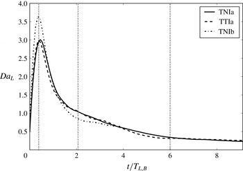
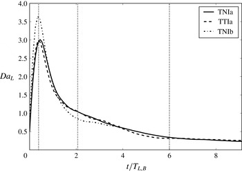
As we have stated at the beginning of § 3.1, the mixing process is transient over the whole period, which implies that the turbulence time scales keep changing. Therefore, in table 3 we have listed times that are either based on initial conditions or taken at time instants indicated in figure 3. In order to get a better idea about the transient character of the mixing process, we show in figure 5 the Damköhler number as a function of time for the three different runs. The Damköhler number relates a fluid time scale to a reaction (or evaporation) time scale. Based on the large-eddy turnover time, it is given by

Equation (3.6) is based on the cloudy half of the slab, $V_{1}$ . We observe in figure 5 that the values of $Da_{L}(t)$ exceed unity by almost a factor of 4 in magnitude in the initial stage of the evolution. The bigger the simulation domain, the larger the local maximum in $Da_{L}(t)$ . This means that the dynamical process leads to a transient inhomogeneous mixing regime (Lehmann et al. Reference Lehmann, Siebert and Shaw2009). Our results suggest that this regime becomes increasingly important as the size of the computational domain grows. Figure 6 shows a vertical cut in TNIb for two instants. The inhomogeneous mixing becomes visible. Domains inside the cloud that are still unaffected by the entrainment coexist with domains that are already strongly mixed.

3.3 Time evolution of plane-averaged profiles across the mixing layer

In order to understand the temporal behaviour of the TKE and the other quantities better, we refine our analysis by averaging over the two statistically homogeneous space directions and studying the profiles along the inhomogeneous $x$ direction. Therefore we average with respect to the vertical $y$ – $z$ planes, i.e. planes that are parallel to the interface. The profiles are denoted by $\langle \cdot (x)\rangle _{yz}$ . Figure 7 shows profiles of buoyancy $B$ (a,b), liquid water mixing ratio $q_{l}$ (c,d) and convective buoyancy flux (e,f) at different times as indicated in the legend.

Figure 7.

Evolution of plane-averaged profiles of (a,b) buoyancy $\langle B(x)\rangle _{yz}$ , (c,d) liquid water content $\langle q_{l}(x)\rangle _{yz}$ and (e,f) production of TKE $\langle u_{z}B(x)\rangle _{yz}$ due to buoyancy. (a,c,e) For case TNIa, and (b,d,f) for case TTIa as summarized in table 1. The dashed lines in the plots are added as a guide to the eye.

Our simulation resembles the situation of a dissolving cloud with negative buoyancy in the cloud core, which is established here solely by the initially added droplets. The cases TNIa (a,c,e) and TTIa (b,d,f) are compared. At the initial stage the cloud slab contains all the droplets and those that are near the interface start to evaporate slowly. Therefore, negative buoyancy is enhanced at the cloud–clear air interface, visible as new local minima in the buoyancy profile. These minima are more pronounced for TNIa. Here, cloud droplets enter an environment with a significantly lower TKE and are decelerated compared to TTIa. For the latter they are advected further due to the same amplitude of velocity fluctuations in- and outside the cloud. The TKE contrast in case TNIa accelerates the decoupling of droplets due to gravitational settling and thus results in larger contributions to $B=-gq_{l}$ (see (2.5)). This causes the slightly larger magnitudes of $\langle B(x)\rangle _{yz}$ when TNIa is compared to TTIa in figure 7(a,b).

The profiles confirm also that the TTI set-up enhances entrainment for times larger than $T_{L,B}$ (see also table 3). This can be clearly seen in the liquid water profiles $\langle q_{l}(x)\rangle _{yz}$ , e.g. by a comparison at $t=32$ s or $4\,T_{L,B}$ . In the TTIa case, the liquid water content is significantly reduced compared with TNIa at the same time $t$ . The stronger buoyancy minimum at the interface and the reduced lateral transport are responsible for a stronger TKE production due to the convective buoyancy flux $\langle u_{z}B(x)\rangle _{yz}$ , as seen in figure 7(e,f). The role of evaporative cooling for the generation of TKE has been stressed by Malinowski et al. (Reference Malinowski, Andrejczuk, Grabowski, Korczyk, Kowalewski and Smolarkiewicz2008) and Mellado (Reference Mellado2010), and we see that this indeed is a dominant factor in the evolution, especially for the shearless mixing layer TNIa.

3.4 Growth of the mixing layer

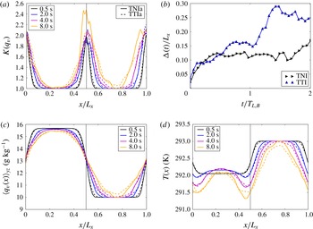
Since the cloud–clear air interface is not resolved in most large-eddy simulations of turbulent clouds, the growth of the mixing layer has to be modelled. In this subsection, we determine this growth of the mixing layer from our simulation data. This provides a measure for the entrainment velocity. We will use here the kurtosis of the vapour mixing ratio field to quantify the growth. This positive definite quantity is exactly one in the unmixed regions inside and outside the cloud and larger than one in regions where the mixing and entrainment proceeds. Other measures based on vorticity are possible as discussed for example in the review by da Silva et al. (Reference da Silva, Hunt, Eames and Westerweel2014). Specifically, we calculate

and show the resulting profiles in figure 8(a,c). Again, cases TNIa and TTIa are compared. The width of the mixing layer is taken as the width of the profile at half the maximum. It is denoted by $\unicode[STIX]{x1D6E5}(t)$ and shown in figure 8(b). The width remains comparable during the first stage of the mixing process. With the beginning of the second phase for times $t\gtrsim 0.5T_{L,B}$ , we observe that the width of the layer grows faster for TTI, which is consistent with the more rapid increase of the mean vapour content in § 3.1. One may conclude, therefore, that the early progression of the mixing process is dominated by the eddy structure in the cloudy region, with relatively small differences between TNIa and TTIa, but at larger times the evolution diverges due primarily to the differing TKE levels.

Figure 8.

Growth of the mixing layer with respect to time. (a) Evolution of the kurtosis $K(q_{v})$ as a function of time. (b) Growth of the width of the mixing layer, $\unicode[STIX]{x1D6E5}(t)$ , with respect to time. Again the two cases TNIa and TTIa are compared. The time axis is rescaled by the corresponding large-eddy turnover time $T_{L,B}$ , which is 7.7 s in case TNIa and 9.1 s for TTIa. For comparison we show the profiles of plane-averaged vapour mixing ratio (c) and temperature (d).

3.5 Enstrophy and shear production in the mixing layer

As we showed in § 3.3, the negative buoyancy due to evaporative cooling generates kinetic energy. A shear layer is formed in the interface region, which generates a dominantly upward motion outside the cloud and downward motion inside the cloud. These shear layers are a main source for enhanced turbulent fluctuations and thus for kinetic energy dissipation. In order to study this aspect in more detail, we display in figure 9 isosurfaces of the local enstrophy and the kinetic energy dissipation fields. The vorticity is given by

with $\unicode[STIX]{x1D716}_{ijk}$ being the Levi-Civita symbol. The local enstrophy is the squared magnitude of the vorticity, $\unicode[STIX]{x1D714}^{2}=\unicode[STIX]{x1D714}_{i}\unicode[STIX]{x1D714}_{i}$ . The kinetic energy dissipation rate field is defined in (3.2). We recall that the two ensemble averages are connected in homogeneous isotropic turbulence by

Figure 9.

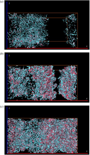
Isosurfaces of the local enstrophy (blue) and kinetic energy dissipation (red) for different times. Times are $t\approx 4~\text{s}$ (a), $t\approx 16~\text{s}$ (b) and $t\approx 32~\text{s}$ (c). The view is on the front face of the domain. Initially, the cloudy fraction occupies the left half of the box. Data are for run TNIb. The isolevels for the three panels are $\unicode[STIX]{x1D716}=32~\text{cm}^{2}~\text{s}^{-3}$ and $\unicode[STIX]{x1D714}^{2}=213~\text{s}^{-2}$ such that $\unicode[STIX]{x1D716}=\unicode[STIX]{x1D708}\unicode[STIX]{x1D714}^{2}$ . Times correspond to 0.4, 1.6 and 3.1 eddy turnover times  $T_{L,B}$ .

Isolevels of both fields are shown at a fixed value for all three time instants. The snapshots are taken at times $t\approx 4~\text{s}$ , $t\approx 16~\text{s}$ and $t\approx 32~\text{s}$ (or approximately 0.4, 1.6 and $3.1\,T_{L,B}$ ) for the biggest shearless mixing layer run, TNIb. Initially, fine-scale structures of both quantities are visible primarily in the left part of the box in which the TKE has a larger amplitude. As the turbulence decays, smaller eddies are dissipated, leading to coarser structures. Owing to evaporative cooling, up- and downdraughts are generated, producing the largest shear and vorticity events at the interface, as is visible in figure 9(b). In figure 9(c) it is clearly visible that, in the later stage of the evolution, the high-amplitude events are now located in- and outside the original cloud location. At time $t=32~\text{s}$ the droplets have spread into the clear air region, and have evaporated and generated smaller flow structures due to evaporative cooling and gravitational settling. This now generates most of the dissipation and local enstrophy. Figure 9 shows that the isocontours of energy dissipation and local enstrophy are always found together, a result which is known from other flows such as homogeneous isotropic turbulence (Schumacher, Eckhardt & Doering Reference Schumacher, Eckhardt and Doering2010). The levels of both isocontours have been chosen such that $\unicode[STIX]{x1D716}=\unicode[STIX]{x1D708}\unicode[STIX]{x1D714}^{2}$ . The exact relation (3.9) for the mean values of both fields is also locally quite well established.

The production of shear and vorticity can be discussed by means of the balance equations for shear magnitude and local enstrophy. The vorticity equation follows from (2.2) as

with an additional term due to buoyancy on the right-hand side. It results in a balance for the local enstrophy of

The evolution of the $ij$ component of the rate-of-strain tensor is given by

A similar balance as for the local enstrophy follows for the magnitude square of the strain $S^{2}=\unicode[STIX]{x1D61A}_{ij}\unicode[STIX]{x1D61A}_{ji}$ , given by

where the pressure Hessian $P_{ij}$ is defined as

Equation (3.11) contains the enstrophy production term $P_{\unicode[STIX]{x1D714}S}=2\unicode[STIX]{x1D714}_{i}\unicode[STIX]{x1D61A}_{ij}\unicode[STIX]{x1D714}_{j}$ due to vortex stretching. This term enters also the strain production balance in (3.13), which is given by $P_{S}=-2\unicode[STIX]{x1D61A}_{ij}\unicode[STIX]{x1D61A}_{jk}\unicode[STIX]{x1D61A}_{ki}-\unicode[STIX]{x1D714}_{i}\unicode[STIX]{x1D61A}_{ij}\unicode[STIX]{x1D714}_{j}/2$ . Both equations contain production terms due to the buoyancy feedback, $P_{\unicode[STIX]{x1D714}B}=2\unicode[STIX]{x1D716}_{zik}\unicode[STIX]{x1D714}_{i}\unicode[STIX]{x2202}_{k}B$ in (3.11) and $P_{SB}=2\unicode[STIX]{x1D61A}_{zi}\unicode[STIX]{x2202}_{i}B$ in (3.13). The non-local pressure–strain coupling is not investigated more closely here as well as the dissipative terms in both balance equations.

Figure 10.

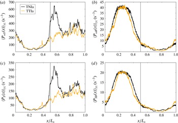
Production of enstrophy and strain in the mixing layer. Similar to figure 7, we display profiles that are obtained by averages over $y$ – $z$ planes at time $t=16~\text{s}$ . (a) Enstrophy production due to vortex stretching, $P_{\unicode[STIX]{x1D714}S}$ . (b) Enstrophy production due to buoyancy, $P_{\unicode[STIX]{x1D714}B}$ . (c) Strain production due to strain–strain coupling. (d) Strain production due to buoyancy, $P_{SB}$ .

Figure 11.

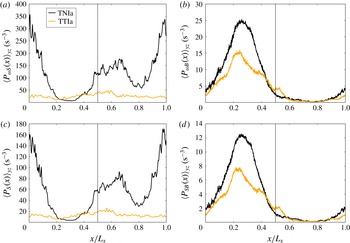
Same data as in figure 10 for $t=32~\text{s}$ .

In figures 10 and 11 we analyse the different production terms that appear in (3.11) and (3.13). Averages over $y$ – $z$ planes versus the $x$ coordinate perpendicular to the initial cloud–clear air interface are shown again. Figure 10 is taken at $t=16~\text{s}$ and figure 11 at $t=32~\text{s}$ . Panels (a,c) in figures 10 and 11 display the production terms, $P_{\unicode[STIX]{x1D714}S}$ and $P_{S}$ , and panels (b,d) show enstrophy and strain production due to the coupling between buoyancy and the vertical velocity component, $P_{\unicode[STIX]{x1D714}B}$ and $P_{SB}$ . In Schumacher, Götzfried & Scheel (Reference Schumacher, Götzfried and Scheel2015) it was shown that $P_{\unicode[STIX]{x1D714}B}\ll P_{\unicode[STIX]{x1D714}S}$ for standard Rayleigh–Bénard convection. This result can be confirmed here and even extended to the strain balance. Furthermore, it can be seen that there are significant differences between cases TNIa and TTIa. They become larger as the time proceeds and are strongest for $P_{\unicode[STIX]{x1D714}S}$ and $P_{S}$ , respectively. For $t=16~\text{s}$ , the strong peak of $P_{\unicode[STIX]{x1D714}S}$ and $P_{S}$ at the interface is absent in the case of TTIa, in which no gradient of turbulence intensity exists. A $t=32~\text{s}$ , case TTIa obeys an almost homogeneous production profile for $P_{\unicode[STIX]{x1D714}S}$ and $P_{S}$ . Furthermore, both buoyancy production terms are significantly smaller in amplitude.

The profiles of $P_{\unicode[STIX]{x1D714}S}$ and $P_{S}$ are almost identical and differ in magnitude only. The same holds for $P_{\unicode[STIX]{x1D714}B}$ when compared with $P_{SB}$ . Both reflect the tight interplay between strain and enstrophy generation. Furthermore, figures 10 and 11 show that the small-scale turbulence is strongly altered when the turbulence levels inside and outside the cloud differ, a result that was much less clearly visible from macroscopic quantities that we have compared in the preceding sections. Our studies show that the local strain and enstrophy production are mostly caused by the nonlinear coupling of the fluid turbulence, which however has its origin in the buoyancy feedback.

4.1 Droplet trajectories at the interface

In figure 6 we saw that a subset of the droplets remains for a long time inside the cloud core while other subsets at the cloud edge have already been completely evaporated. This is the central idea of an inhomogeneous mixing scenario.

Figure 12.

Droplet trajectories and plots of the corresponding temperature $T$ , supersaturation $S$ and vertical velocity $V_{z}$ along the droplet paths for the cases where droplets evaporate fast (a,d,g,j), return back to the initial cloud domain (b,e,h,k) or stay inside the cloud (c,f,i,l). The plane in the trajectory plots marks the initial interface between cloudy and clear air subdomains. Data are obtained from TNIa. Thin solid lines in trajectory plots indicate droplets that are practically evaporated.

In the following we extract such subsets of particles and examine the thermodynamic properties along their trajectories. Therefore, we divide the droplets into three categories: droplets that evaporate very quickly by entering the subsaturated cloud environment immediately; droplets that enter the subsaturated area and return back into the cloud filament; and droplets that remain inside the cloud core for a long time. In order to track any given particle location and its thermodynamic properties, we saved the quantities with a time resolution of $\unicode[STIX]{x0394}t=0.05~\text{s}$ . Typical particle trajectories and thermodynamic properties such as temperature $T$ , supersaturation $S$ and vertical droplet velocity component $V_{z}$ are displayed in figure 12 for TNIa. The trajectories are plotted until a time $t=5~\text{s}$ , which corresponds to $0.65\,T_{L,B}$ .

The most interesting case is shown in figure 12(b,e,h,k), where particles enter the subsaturated region and then return back into the cloudy region. On their way they experience temperatures below the initial cloud temperature of $T_{c}=292.0~\text{K}$ . Being initially in a strongly subsaturated state, they return back to a more humid environment that is still subsaturated. This is sufficient for the droplets to fully evaporate although they again enter the cloud interface. Droplets inside the cloud core as shown by figure 12(c,f,i,l) are moving downwards with negative vertical velocity due to the overall drag included in the buoyancy, as given by (2.5). Initially they are in a supersaturated state and can grow in radius by condensation. This is visible by a slight temperature increase since latent heat is released. The supersaturation decays slowly exponentially to values close to zero. This subset represents the majority of cloud droplets, where the initial profile of the rescaling function was constant. Some droplets at the cloud edge enter the subsaturated area immediately as shown in figure 12(a,d,g,j). Initially, a jump in all thermodynamic values is visible where droplets change from positive vertical velocity suddenly to negative values. This sudden changes occur as particles pass the interface. Once they are evaporated and far away from the interface, they experience a positive updraught.

4.2 Distribution of droplet size and supersaturation

Cloud droplet radius evolves in time as mixing progresses and, until complete evaporation occurs, the supersaturation and the temperature at the droplet positions will also vary in time. Prior Lagrangian simulations of mixing at the edge of a cloud by Kumar et al. (Reference Kumar, Janetzko, Schumacher and Shaw2012, Reference Kumar, Schumacher and Shaw2014) and Perrin & Jonker (Reference Perrin and Jonker2015) showed that entrainment of subsaturated air leads to a broadening of the particle size distribution with extended exponential tails to smaller radii. The growth of the droplet radii and thus the broadening of the tail on the right side of the droplet size distribution can proceed only for an initial period deep inside the cloud where supersaturation is positive. It remains a small effect in our study. In order to focus on the microphysical response to mixing, we do not include a supersaturation forcing term (Lanotte et al. Reference Lanotte, Seminara and Toschi2009) and collisions and coalescence (Perrin & Jonker Reference Perrin and Jonker2015).

Figure 13.

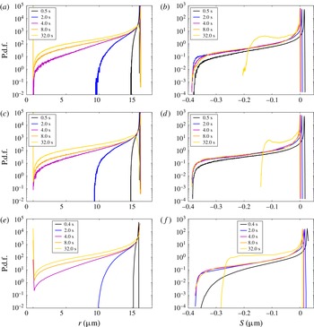
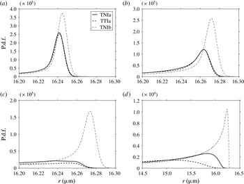
(a,c,e) Probability density functions (p.d.f.s) of cloud water droplet radius at different times are plotted for TNIa (a), TTIa (c) and TNIb (e). (b,d,f) The p.d.f.s of supersaturation at the same time instants, again for TNIa (b), TTIa (d) and TNIb (f).

Figure 14.

Zoomed view of the maximum of the droplet size distribution for the three runs at different times: (a) $t=4~\text{s}$ ; (b) $t=8~\text{s}$ ; (c) $t=16~\text{s}$ ; (d) $t=32~\text{s}$ . The line styles for the different curves are indicated in the legend.

Figure 13(a,c,e) shows the probability density function (p.d.f.) of the droplet radius for simulations TNIa (a), TTIa (c) and TNIb (e). Data are taken for the whole simulation domain. The comparison between TNIa and TTIa shows that slight differences occur in the evolution of the small droplet tail, with faster development occurring in the fully turbulent domain (TTIa). The comparison with TNIb shows that an increased size of the simulation domain and therefore of the Reynolds number leads to a somewhat slower growth of the left tail of the droplet size distribution. This is a result of the large-eddy turnover time for TNIb being greater than that for TNIa. The differences in the size distributions are more evident in the zoomed plots shown in figure 14, in which we resolve, for different times, the peak of the distributions and the right tail where the largest droplets are observed. Here we clearly see that the differences between TNIa and TTIa are indeed small except for the last time. Presumably this is a result of the differing turbulence intensities in the two cases for times large compared to their corresponding eddy turnover time. The change in microphysical response as the computational domain size is increased (TNIa versus TNIb) is especially evident in this zoomed plot. The droplet size distribution remains much narrower in the larger domain, which is closer to the limit of extreme inhomogeneous mixing, i.e. the radius of most of the droplets remains unchanged for a longer time period during the mixing process. Figure 13(b,d,f) shows the p.d.f.s of supersaturation at the droplet locations (2.12) for the same simulation runs and the same times. They confirm that the majority of droplets remain close to the nearly saturated state ( $S=0$ ), with an exponential tail of subsaturated conditions. As with the droplet radius, slight differences in the left tails can be seen for TNIa and TTIa, especially at long times when the turbulence intensities are different. The same can be seen when TNIb is compared with TNIa. Here the reason is the larger domain, which leaves larger fractions of the cloud cores unmixed in the early stage, and in which mixing progresses more slowly due to the increase in large-eddy turnover time (see also figure 6).

Figure 15.

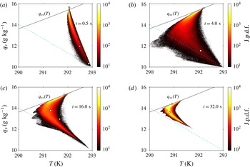
Time evolution of joint p.d.f. distribution for temperature $T$ and water vapour mixing ratio $q_{v}$ at the droplet positions, shown only for case TNIa. The solid line displays the dependence of the saturation vapour mixing ratio on temperature. The dashed line connects the initial state of the warmer cloud environment ( $q_{ve}(t=0),T_{e}(t=0)$ in the lower right with the point $(q_{vs}(T_{\infty }),T_{\infty })$ . The triangles, squares and circles in the plots represent the thermodynamic state of three representative droplets, which evaporate very quickly outside the cloud, re-enter the cloudy domain and remain in the cloud core, respectively. Times correspond to approximately 0.07, 0.5, 2 and 4 eddy turnover times $T_{L,B}$ .

4.3 Droplet ensemble in temperature–vapour parameter plane

The Lagrangian evolution of the droplet ensemble will now be displayed in a parameter plane that is spanned by vapour content and temperature. In this way, we provide a complementary view of the evolution of mixing that has been discussed in § 3.3 on the basis of plane-averaged profiles. We will also provide a connection to the three individual trajectories that have been examined in detail in § 4.1.

Figure 15 shows the joint probability density function (j.p.d.f.) of vapour mixing ratio $q_{v}$ and temperature $T$ taken at the particle positions for the TNIa case only; we saw that the TTIa case showed quite similar results. As already stated, the existence of a large latent heat leads to a decrease in the temperature $T$ locally during droplet evaporation. The temperature decrease and the increase of water vapour content that occur during mixing and droplet evaporation are important to consider in detail because they both feed back to the flow via buoyancy, leading to vertical acceleration of the fluid. The solid line drawn in all the panels of figure 15 represents the saturation vapour mixing ratio, $q_{vs}(T)$ , which is given by (2.13). Except for the early stage (see figure 15 a for $t=0.5$  s), the saturation threshold is not exceeded by the majority of the droplets. As the time proceeds, the distribution as a whole converges to the $q_{vs}(T)$ line while spreading to lower temperatures. This line therefore marks the upper bound approached by all droplets as the mixing progresses. The dashed line in all the panels of figure 15 connects the initial state of the warmer clear air environment with $q_{ve}(t=0)=0.01$ and $T_{e}(t=0)=293~\text{K}$ in the lower right, with the end point of the mixing process, $(q_{vs}(T_{\infty }),T_{\infty })$ in the upper left (where the two lines cross). Again, we observe how the j.p.d.f. converges to this line as well, forming all together a shape that is similar to a swept wing. With progressing time, the j.p.d.f. contracts towards $(q_{vs}(T_{\infty }),T_{\infty })$ .

We note that the temperature of the droplets growing by diffusion in the cloud core is slightly increased within the first large-eddy turnover times, up to times of approximately $t=16~\text{s}$ or $t\approx 2\,T_{L,B}$ . This result of latent heat release competes with the overall mixing to result in the peak of the j.p.d.f. being stretched along the $q_{vs}(T)$ line during the first few eddy turnover times. Interestingly, the small subset of droplets that experiences sudden evaporative cooling at the cloud–clear air interface reach temperatures even lower than those at the dashed line. Their temperature decreases to values as small as $T=290~\text{K}$ . This is most visible in figure 15(b,c). Although not shown here, this is a result of a strong evaporative cooling of droplets that fall into regions of dry air due to gravitational settling. In figure 15(d) at time $t=32~\text{s}$ , the tail towards the clear air condition has become well aligned with the dashed line. We also note that the maximum temperature of $T_{e}=293~\text{K}$ is consistently not exceeded. This is the initial clear air temperature with lower vapour concentration. All droplets that enter the environment can only shrink and consume heat.

Although not shown here, the same qualitative behaviour follows for TNIb except more slowly in time. Here, again, owing to finite computational resources, we could not run the simulation long enough to approach the final mixing state. Owing to the larger domain size, this state will be reached in TNIb later than in TNIa. Again, the growth process of the droplets and thus the increase of the most probable temperature in the core proceeds for somewhat longer since the supersaturated domain is bigger.

4.4 Joint Lagrangian statistics of local dissipation rate and local enstrophy

In order to obtain further quantitative insight on the joint statistics of local enstrophy and kinetic energy dissipation rate fields, we display the j.p.d.f. for TNIa at two different instants in figure 16. In detail, we plot

which normalizes the j.p.d.f. of $\unicode[STIX]{x1D716}$ and $\unicode[STIX]{x1D714}^{2}$ by the corresponding single-quantity p.d.f.s in order to highlight the correlation of far tail events better. As the two panels of figure 16 show, particularly very-low- and very-high-amplitude dissipation and local enstrophy events are found in close vicinity to each other. This holds for the whole dynamical evolution of the mixing process and for all runs considered. The bimodal and skewed shape of $\unicode[STIX]{x1D6F1}$ agrees with those of numerical simulations of box turbulence by Schumacher et al. (Reference Schumacher, Eckhardt and Doering2010) and grid turbulence experiments by Zeff et al. (Reference Zeff, Lanterman, McAllister, Roy, Kostelich and Lathrop2003). In fluid turbulence, the highest-enstrophy events are generated by vortex stretching. This stretching of a vortex tube always induces strain and thus energy dissipation around the stretched tube as a nonlinear feedback that reduces the original background strain that is responsible for the stretching. This mechanism was studied in detail, for example, in Hamlington, Schumacher & Dahm (Reference Hamlington, Schumacher and Dahm2008) and explains why local maxima of dissipation and enstrophy are found in close vicinity.

Figure 16.

Joint p.d.f.s of kinetic energy dissipation rate and local enstrophy for the whole box in the Lagrangian frame of reference: (a)  $t=0.5~\text{s}$ ; (b)  $t=16~\text{s}$ . Data are for the TNIa case. Both joint distributions are normalized by the corresponding single-particle p.d.f.s.