1. Introduction
Among wall-bounded turbulent flows, a plane turbulent wall jet captivates researchers due to its intricate and intriguing flow characteristics, as well as its wide spectrum of engineering applications. It plays a key role in industrial and aerospace systems, including automobile windscreen defrosters, separation control on aircraft wings, film cooling mechanisms in combustion chambers and leading-stage blades of gas turbines (Launder & Rodi Reference Launder and Rodi1983). Since the seminal work of Förthmann (Reference Förthmann1934), plane turbulent wall jets have been extensively studied theoretically (Glauert Reference Glauert1956; Narasimha, Narayan & Parthasarathy Reference Narasimha, Narayan and Parthasarathy1973; Hammond Reference Hammond1982; George et al. Reference George, Abrahamsson, Eriksson, Karlsson, Löfdahl and Wosnik2000; Afzal Reference Afzal2005; Barenblatt, Chorin & Prostokishin Reference Barenblatt, Chorin and Prostokishin2005; Afzal & Seena Reference Afzal and Seena2011,Reference Afzal and Seena2013; Gersten Reference Gersten2015; Djenidi & Agrawal Reference Djenidi and Agrawal2024), experimentally (Sigalla Reference Sigalla1958; Schwarz & Cosart Reference Schwarz and Cosart1961; Bradshaw & Gee Reference Bradshaw and Gee1962; Myers, Schauer & Eustis Reference Myers, Schauer and Eustis1963; Tailland & Mathieu Reference Tailland and Mathieu1967; Irwin Reference Irwin1973; Wygnanski, Katz & Horev Reference Wygnanski, Katz and Horev1992; Karlsson et al. Reference Karlsson, Eriksson and Persson1993a , Reference Karlsson, Eriksson and Perssonb ; Schneider & Goldstein Reference Schneider and Goldstein1994; Eriksson, Karlsson & Persson Reference Eriksson, Karlsson and Persson1998; Tachie Balachandar & Bergström Reference Tachie, Balachandar and Bergstrom2002, Reference Tachie, Balachandar and Bergstrom2004; Smith Reference Smith2008; Rostamy et al. Reference Rostamy, Bergstrom, Sumner and Bugg2011a , Reference Rostamy, Bergstrom, Sumner and Buggb ; Tang et al. Reference Tang, Rostamy, Bergstrom, Bugg and Sumner2015,Reference Tang, Bergstrom and Bugg2017; Gnanamanickam et al. Reference Gnanamanickam, Bhatt, Artham and Zhang2019; Kleinfelter et al. Reference Kleinfelter, Repasky, Hari, Letica, Vishwanathan, Organski, Schwaner, Alexander and Devenport2019; Mcintyre et al. Reference Mcintyre, Savory, Wu and Ting2019; Gupta et al. Reference Gupta, Choudhary, Singh, Prabhakaran and Dixit2020; Wei, Wang & Yang Reference Wei, Wang and Yang2021; Choudhary et al. Reference Choudhary, Gupta, Bhatt, Prabhakaran, Singh, Karipot and Dixit2024; Sood et al. Reference Sood, Bhatt, Choudhary, Gupta, Raghuvanshi, Sapkal, Prabhakaran and Dixit2025) and numerically (Dejoan & Leschziner Reference Dejoan and Leschziner2005; Levin et al. Reference Levin, Chernoray, Löfdahl and Henningson2005,Reference Levin, Herbst and Henningson2006; Ahlman, Brethouwer & Johansson Reference Ahlman, Brethouwer and Johansson2007; Banyassady & Piomelli Reference Banyassady and Piomelli2014,Reference Banyassady and Piomelli2015; Naqavi, Tyacke & Tucker Reference Naqavi, Tyacke and Tucker2018). Comprehensive studies on the topic were compiled by Rajaratnam (Reference Rajaratnam1976) and Launder & Rodi (Reference Launder and Rodi1979,Reference Launder and Rodi1983).
Figure 1(a) presents a sketch of a plane turbulent wall jet originating from a source. Experimental studies have shown that a turbulent wall jet becomes fully developed when x/b exceeds 30 (Narasimha et al. Reference Narasimha, Narayan and Parthasarathy1973; Eriksson et al. Reference Eriksson, Karlsson and Persson1998). Here, x is the streamwise distance and b is the source thickness. The streamwise velocity profile
 $\overline{u}(z)$
in the fully developed region exhibits a non-monotonic velocity profile (figure 1
a), distinguishing plane turbulent wall jets from other wall-bounded turbulent flows. The local velocity attains a maximum, called the jet velocity U
m
, at a wall-normal location z = z
m
, and decreases on either side of z = z
m
. Another important length parameter is the jet half-width z
1/2, defined as the wall-normal location where the local velocity above z = z
m
drops to U
m
/2. In the fully developed region, key jet parameters, such as the jet velocity U
m
, jet half-width z
1/2 and wall shear stress
 $ \tau_{0}$
, vary with the streamwise distance. Moreover, following the study of George et al. (Reference George, Abrahamsson, Eriksson, Karlsson, Löfdahl and Wosnik2000), figure 1(b) illustrates a conceptual sketch of various flow layers across the jet using the dimensionless wall-normal coordinates z/z
1/2 and z
+ = zu
*/
 $v$
, where u
* is the friction velocity and
 $v$
is the coefficient of kinematic viscosity of fluid. The flow layers include the viscous sublayer (z
+ < 3), buffer layer (3 < z
+ < 30), mesolayer (30 < z
+ < 300), inertial sublayer (300 < z
+< 0.1
 $z_{1/2}^{+}$
) and outer layer (z/z
1/2 > 0.1). The mesolayer and the inertial sublayer form the overlap region (30 < z
+ < 0.1
 $z_{1/2}^{+}$
).
(a) Schematic illustration of the plane turbulent wall jet evolving in the streamwise direction x. The jet originates from a source of thickness b with an exit velocity U
0 at x = 0. The streamwise velocity profile
 $\overline{u}(z)$
is depicted in the fully developed region. Here, U
m
is the jet velocity at z = z
m
and z
1/2 is the jet half-width, where the velocity above z = z
m
reduces to U
m
/2. The red dashed line indicates the wall-normal location z = z
m
, which corresponds to the jet velocity U
m
. (b) Conceptual sketch of various flow layers (George et al. Reference George, Abrahamsson, Eriksson, Karlsson, Löfdahl and Wosnik2000).

In a fully developed plane turbulent wall jet, the relevant scaling parameters for U
m
, z
1/2 and
 $ \tau_{0}$
are the kinematic momentum flux M and the coefficient of kinematic viscosity of fluid
 $v$
. With regard to M, three approaches are available, as briefly outlined below.
-
(i) Source approach: the most commonly used approach in the literature is based on the initial condition. It considers the source kinematic momentum flux, M = M 0 =
 $U_{0}^{2}$
b, as the scaling parameter (Narasimha et al. Reference Narasimha, Narayan and Parthasarathy1973; Wygnanski et al. Reference Wygnanski, Katz and Horev1992).
-
(ii) Asymptotic approach: this approach is based on the asymptotic far-downstream condition, where the wall jet is considered to asymptotically approach a half-free jet as the Reynolds number tends to infinity (Gersten Reference Gersten2015). The asymptotic kinematic momentum flux, M =
$M_{\infty}$
is considered as the scaling parameter. However, Gersten (Reference Gersten2015) noted that this approach is invalid for wall jets emerging from a wall perpendicular to the inflow velocity vector. -
(iii) Local approach: this method considers the local kinematic momentum flux, M = M l =
$\int _{0}^{\infty }\overline{u}^{2}\mathrm{d}z$
, as the scaling parameter (Gupta et al. Reference Gupta, Choudhary, Singh, Prabhakaran and Dixit2020). Gupta et al. (Reference Gupta, Choudhary, Singh, Prabhakaran and Dixit2020) argued that since the notion of self-similarity is inherently a local concept, this approach is more appropriate than the source and asymptotic approaches.


Gupta et al. (Reference Gupta, Choudhary, Singh, Prabhakaran and Dixit2020) scrutinised the aforementioned three approaches using experimental data from the literature. They found that, overall, the local approach yields superior data collapse for U
m
, z
1/2 and
 $ \tau_{0}$
. This conclusion was drawn based on the root-mean-square error (RMSE) analysis of the experimental data fits, wherein the local approach produced the lowest RMSE (except in the case of z
1/2 data) among the three approaches. Moreover, the data plots were found to follow the local scaling based on M = M
l
and
 $v$
, regardless of whether the wall jet originates from a wall perpendicular to the inflow velocity vector. This innovative approach has advanced the understanding of the relevant scaling laws. However, with regard to the asymptotic and local approaches, determining
 $M_{\infty}$
and M
l
remains challenging. While
 $M_{\infty}$
is derived from asymptotic, far-downstream analysis (Gersten Reference Gersten2015), calculating M
l
requires the time-averaged streamwise velocity profiles at various streamwise distances (Gupta et al. Reference Gupta, Choudhary, Singh, Prabhakaran and Dixit2020). Given these complexities, the present study specifically considers the source approach, where the source kinematic momentum flux M
0 is straightforward to determine without additional effort. Using this scaling framework, dimensional analysis provides the following forms for U
m
, z
1/2 and
 $ \tau_{0}$
:
 \begin{align} \frac{U_{m}v }{M_{0}}&=f_{1}\left(\frac{{\textit{xM}}_{0}}{{v} ^{2}},{\textit{Re}}_{\!j}\right)\! , \end{align}
 \begin{align} \frac{z_{1/2}M_{0}}{{v} ^{2}}&=f_{2}\left(\frac{{\textit{xM}}_{0}}{{v} ^{2}},{\textit{Re}}_{\!j}\right)\! , \end{align}
 \begin{align} \frac{\tau _{0}{v} ^{2}}{\rho M_{0}^{2}}&=f_{3}\left(\frac{{\textit{xM}}_{0}}{{v} ^{2}},{\textit{Re}}_{\!j}\right)\! , \end{align}
where f
1, f
2 and f
3 are the mathematical functions, Re
j
= U
0
b/
 $v$
is the source Reynolds number and ρ is the mass density of fluid.
Barenblatt et al. (Reference Barenblatt, Chorin and Prostokishin2005) argued that the influence of source thickness b, or equivalently the impact of Re
j
, never vanishes. This yields incomplete similarity. Applying their mathematical framework to the present problem, U
m
and z
1/2 can be expressed as functions of the independent parameters x, b, M
0 and
 $v$
. Accordingly, U
m
= U
m
(x, b, M
0,
 $v$
) and z
1/2 = z
1/2(x, b, M
0,
 $v$
). Since this framework considers b and
 $v$
as the relevant scaling parameters, dimensional analysis for U
m
yields the Π parameters as Π
1 = U
m
b/
 $v$
, Π
2 = x/b and Π
3 =
 $\sqrt{M_{0}b/v ^{2}}$
= Re
j
. Taking the ratio Π
1/Π
3 = U
m
/U
0, the functional relationship leads to U
m
/U
0 = f
4(x/b, Re
j
), where f
4 is a functional form. A similar analysis for z
1/2 gives z
1/2/b = f
5(x/b, Re
j
), where f
5 is the corresponding function. The incomplete similarity implies that, for both functional relationships, U
m
/U
0 = f
4(x/b, Re
j
) and z
1/2/b = f
5(x/b, Re
j
), the influence of Re
j
remains important. This suggests that the experimental data of U
m
/U
0 or z
1/2/b plotted against x/b do not collapse on a single band for different Re
j
. This lack of data collapse for U
m
/U
0 versus x/b and z
1/2/b versus x/b was identified by Narasimha et al. (Reference Narasimha, Narayan and Parthasarathy1973) and George et al. (Reference George, Abrahamsson, Eriksson, Karlsson, Löfdahl and Wosnik2000), thereby substantiating incomplete similarity. However, the incomplete similarity does not necessarily hold if the relevant scaling parameters are chosen more appropriately while remaining within the framework of Barenblatt et al. (Reference Barenblatt, Chorin and Prostokishin2005). For example, the selection of M
0 (instead of b) and
 $v$
as the relevant scaling parameters directly produces the functional forms given in (1.1)–(1.3). Experimental observations have evidenced that the data plots of U
m
 $v$
/M
0 versus xM
0/
 $v$
2, z
1/2
M
0/
 $v$
2 versus xM
0/
 $v$
2 and
 $ \tau_{0}$
 $v$
2/(ρ
 $M_{0}^{2}$
) versus xM
0/
 $v$
2 collapse on a single band for different Re
j
(see figures 7
a, 8
a and 10
a), revealing complete similarity. Gupta et al. (Reference Gupta, Choudhary, Singh, Prabhakaran and Dixit2020) further emphasised that a judicious choice of repeating variables within the framework of Barenblatt et al. (Reference Barenblatt, Chorin and Prostokishin2005) enables complete similarity, indicating that the influence of b or Re
j
becomes vanishingly small. Therefore, (1.1)–(1.3) for large Re
j
yield Re
j
-independent power-law scaling relationships as follows:
 \begin{align} \frac{U_{m}v }{M_{0}}&\sim \left(\frac{{\textit{xM}}_{0}}{{v} ^{2}}\right)^{-\alpha } \!,\end{align}
 \begin{align} \frac{z_{1/2}M_{0}}{{v} ^{2}}&\sim \left(\frac{{\textit{xM}}_{0}}{{v} ^{2}}\right)^{\beta } \!,\end{align}
 \begin{align} \frac{\tau _{0}{v} ^{2}}{\rho M_{0}^{2}}&\sim \left(\frac{{\textit{xM}}_{0}}{{v} ^{2}}\right)^{-\chi } \!,\end{align}
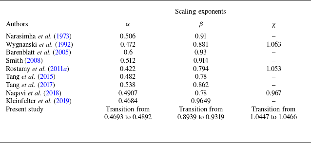
where α, β and χ are the positive scaling exponents, and the symbol ‘∼’ represents ‘scales with’. The power laws (1.4)–(1.6) are supported by experimental observations (see, for instance, Narasimha et al. (Reference Narasimha, Narayan and Parthasarathy1973) and Wygnanski et al. (Reference Wygnanski, Katz and Horev1992)). Various estimates of α, β and χ are available in experimental studies of plane turbulent wall jets.
Despite significant advancements, little attention has so far been paid to deriving the scaling exponents α, β and χ from a theoretical perspective. These exponents have traditionally been determined empirically through regression analyses of the experimental data. As a result, they lack a concrete theoretical foundation. Moreover, all experimental studies to date have considered α, β and χ to be invariant with the streamwise distance. This indicates that, when the experimental data of U
m
 $v$
/M
0, z
1/2
M
0/
 $v$
2 or
 $ \tau_{0}$
 $v$
2/(ρ
 $M_{0}^{2}$
) are plotted against xM
0/
 $v$
2 on logarithmic scales, the data plots collapse on a single band, displaying a constant slope across all values of xM
0/
 $v$
2.
In this study, we develop a theoretical framework to determine the scaling exponents α, β and χ. Beginning with the governing equations and applying the scaling relationships for similarity, we derive an expression for the wall shear stress. Independently, we establish a scaling law of the wall shear stress based on the dynamics of near-wall turbulent eddies. The theoretical framework reveals that the values of α, β and χ are not constant across xM
0/
 $v$
2. Instead, a scaling transition occurs as xM
0/
 $v$
2 increases. This transition arises due to a change in the scaling law of the skin-friction coefficient. We validate our theoretical predictions against the experimental data from the literature.
The rest of the paper is structured as follows. The theoretical analysis is presented in § 2. The theoretical results and comparison of the deduced scaling laws with the experimental data are thoroughly discussed in § 3. Finally, conclusions are drawn in § 4.
2. Theoretical analysis
2.1. Governing equations
For a plane turbulent wall jet, the continuity equation and the streamwise momentum equation are expressed as follows (see, for instance, Rajaratnam Reference Rajaratnam1976):
 \begin{align}& \frac{\partial \overline{u}}{\partial x}+\frac{\partial \overline{w}}{\partial z}=0 , \end{align}
 \begin{align} \overline{u}\frac{\partial \overline{u}}{\partial x}+\overline{w}\frac{\partial \overline{u}}{\partial z}=\frac{1}{\rho }{\cdot }&\frac{\partial \tau }{\partial z}+v \frac{\partial ^{2}\overline{u}}{\partial z^{2}}-\frac{\partial }{\partial x}\left(\overline{u'u'}-\overline{w'w'}\right)\! , \end{align}
where
 $\overline{u}$
and
 $\overline{w}$
are the time-averaged velocity components in the streamwise (x) and wall-normal (z) directions, respectively, τ = −ρ
 $\overline{u'w'}$
is the Reynolds shear stress,
 $u'$
and
 $w'$
are the streamwise and wall-normal velocity fluctuations, respectively, and an overbar represents the statistically time-averaged quantity. The boundary conditions for the above set of equations are the no-slip condition at the wall, that is,
 $\overline{u}$
(x, 0) =
 $\overline{w}$
(x, 0) = 0 and a vanishing streamwise velocity far away from the wall, that is,
 $\overline{u}$
(x, ∞) = 0. The no-slip condition at the wall prevents the possibility of similarity solutions across the entire jet flow layer. The normal stresses in (2.2) are negligible and can therefore be disregarded (George et al. Reference George, Abrahamsson, Eriksson, Karlsson, Löfdahl and Wosnik2000). For a large Reynolds number, (2.2) asymptotically reduces to the outer equation (see figure 1
b)
 \begin{equation} \overline{u}\frac{\partial \overline{u}}{\partial x}+\overline{w}\frac{\partial \overline{u}}{\partial z}=\frac{1}{\rho }{\cdot }\frac{\partial \tau }{\partial z} ,\end{equation}
satisfying the outer boundary condition (
 $\overline{u}$
→ 0 as z → ∞). On the other hand, the inner equation is as follows (see figure 1
b):
 \begin{equation} \frac{\partial }{\partial z}\left(-\overline{u'w'}+v \frac{\partial \overline{u}}{\partial z}\right)=0 ,\end{equation}
where
 $\overline{u}$
(z = 0) = 0. Notably, the integration of (2.4) produces the constant stress layer, given by −
 $\overline{u'w'}$
+
 $v$
∂
 $\overline{u}$
/∂z =
 $u_{*}^{2}$
=
 $ \tau_{0}$
/ρ. The concept of a constant stress layer is questionable in plane turbulent wall jets. Therefore, it is not used in the subsequent analysis.
2.2. Scaling relationships for similarity
This subsection considers the similarity solution for the outer equation in conjunction with the momentum integral equation to obtain an expression for the wall shear stress
 $ \tau_{0}$
. George et al. (Reference George, Abrahamsson, Eriksson, Karlsson, Löfdahl and Wosnik2000) proposed a similarity solution for the outer equation in the limit of infinite Reynolds number. They found that, while the streamwise velocity should be scaled with U
m
, the Reynolds shear stress should be scaled with
 $u_{*}^{2}$
rather than
 $U_{m}^{2}$
. Following this framework, we introduce the functional forms
 \begin{equation}F\!\left(\eta \right)\equiv \frac{\overline{u}}{U_{m}} ,\;G\!\left(\eta \right)\equiv \frac{\tau }{\rho u_{*}^{2}} \;{\rm and}\; \eta \equiv \frac{z}{z_{1/2}} .\end{equation}
Using (2.5), the time-averaged wall-normal velocity is obtained by integrating the continuity equation (see (2.1)) and applying the boundary condition
 $\overline{w}$
(z = 0) = 0. The result is
 \begin{equation} \overline{w}=U_{m}\frac{\mathrm{d}z_{1/2}}{\mathrm{d}x}\left(F\eta -\int _{0}^{\eta }F\mathrm{d}\eta \right)-z_{1/2}\frac{\mathrm{d}U_{m}}{\mathrm{d}x}\int _{0}^{\eta }F\mathrm{d}\eta .\end{equation}
Substituting (2.5) and (2.6) into (2.3) yields the following differential equation for the streamwise momentum balance:
 \begin{equation} \frac{u_{*}^{2}}{U_{m}^{2}}{\cdot }\frac{\mathrm{d}G}{\mathrm{d}\eta }=\left(\frac{z_{1/2}}{U_{m}}{\cdot }\frac{\mathrm{d}U_{m}}{\mathrm{d}x}\right)F^{2}-\left(\frac{\mathrm{d}z_{1/2}}{\mathrm{d}x}+\frac{z_{1/2}}{U_{m}}{\cdot }\frac{\mathrm{d}U_{m}}{\mathrm{d}x}\right)\frac{\mathrm{d}F}{\mathrm{d}\eta }\int _{0}^{\eta }F\mathrm{d}\eta .\end{equation}
The similarity solution is feasible if the terms within the parentheses exhibit the same x-dependence. This condition leads to
 \begin{equation} \frac{\mathrm{d}z_{1/2}}{\mathrm{d}x}\sim \frac{z_{1/2}}{U_{m}}{\cdot }\frac{\mathrm{d}U_{m}}{\mathrm{d}x} ,\end{equation}
which suggests that Um obeys a power law with z 1/2. Using (1.4) and (1.5), we find the exponent of the power law as −α/β. Therefore, we write
 \begin{equation} \frac{U_{m}v }{M_{0}}\sim \left(\frac{z_{1/2}M_{0}}{v ^{2}}\right)^{-\alpha /\beta } .\end{equation}
Subsequently, the scaling constraint (2.9) yields
 \begin{equation} \frac{1}{U_{m}}{\cdot }\frac{\mathrm{d}U_{m}}{\mathrm{d}x}=-\frac{\alpha }{\beta }\left(\frac{1}{z_{1/2}}{\cdot }\frac{\mathrm{d}z_{1/2}}{\mathrm{d}x}\right)\! .\end{equation}
To obtain an expression for
 $ \tau_{0}$
, we perform the momentum integral of (2.2) by neglecting normal stresses and utilising (2.1). This produces
 \begin{equation} \left.\begin{array}{l} \displaystyle \int _{0}^{\infty }\dfrac{\partial \overline{u}^{2}}{\partial x}\mathrm{d}z+\left[\overline{u}\overline{w}\right]_{z=0}^{z=\infty }=-\left(-\overline{u'w'}+v \dfrac{\partial \overline{u}}{\partial z}\right)_{z=0}\\[5pt] \Rightarrow \tau _{0}=-\rho \dfrac{\mathrm{d}}{\mathrm{d}x} \displaystyle \int _{0}^{\infty }\overline{u}^{2}\mathrm{d}z. \end{array}\right\} \end{equation}
Using the function F(η) defined in (2.5), (2.11) is expressed as
 \begin{equation} \tau _{0}=-\rho \frac{\mathrm{d}}{\mathrm{d}x}(U_{m}^{2}z_{1/2})\int _{0}^{\infty }F^{2}\mathrm{d}\eta .\end{equation}
Furthermore, using (2.10), (2.12) produces
 \begin{equation} \tau _{0}=\rho U_{m}^{2}\gamma \frac{\mathrm{d}z_{1/2}}{\mathrm{d}x}\int _{0}^{\infty }F^{2}\mathrm{d}\eta\;\,{\rm with}\,\;\frac{\alpha }{\beta }=\frac{1+\gamma }{2}. \end{equation}
As identified by George et al. (Reference George, Abrahamsson, Eriksson, Karlsson, Löfdahl and Wosnik2000), (2.13) provides an important limiting constraint for α/β. In particular, α/β = 0.5 (that is, γ = 0) represents a vanishing wall shear stress. According to (2.12), γ = 0 necessitates that the term
 $U_{m}^{2}z_{1/2}$
remains constant, consistent with the momentum conservation requirement for a free jet (Rajaratnam Reference Rajaratnam1976). This requirement, however, holds only if there is no momentum transfer to the wall, a situation achievable only at an infinitely large Reynolds number. For finite Reynolds numbers (although sufficiently large), the wall enforces a continual momentum loss, leading to wall shear stress. Since dz
1/2/dx and
 $\int _{0}^{\infty }F^{2}\mathrm{d}\eta$
are positive quantities, (2.13) suggests that γ must be a positive quantity (that is, α/β must be greater than 0.5) to ensure a finite (non-negative) wall shear stress. The determination of γ is described in § 3.3.
2.3. Scaling law of
$ \tau_{0}$

This subsection derives a scaling expression for
 $ \tau_{0}$
, independent of (2.12) or (2.13). The derivation is motivated by the spectral framework of Gioia & Chakraborty (Reference Gioia and Chakraborty2006), linking
 $ \tau_{0}$
to the momentum exchange caused by near-wall turbulent eddies. Although originally proposed for moderate Reynolds number pipe flows, this framework was later extended to extreme Reynolds number flows (Anbarlooei, Cruz & Ramos Reference Anbarlooei, Cruz and Ramos2020). Several improved versions of the framework have also been reported in other flow configurations, such as curved tube flows (Ali & Dey Reference Ali and Dey2024), zero pressure gradient turbulent boundary layer (TBL) flow (Ali & Dey Reference Ali and Dey2022; Anbarlooei, Ramos & Cruz Reference Anbarlooei, Ramos and Cruz2023) and axisymmetric TBL flow (Ali & Dey Reference Ali and Dey2023). Following these developments, this study advances the framework further by systematically extending it to wall jets.
Given that the bulk flow Reynolds number is large, the viscous shear stress remains insignificant. Therefore, the wall shear stress is primarily determined by the magnitude of the Reynolds shear stress in the near-wall flow region. In the enlarged view of the near-wall region (figure 2), the Reynolds shear stress is evaluated at a reference level, denoted as z = z R , with the precise location defined in § 2.4. The Reynolds shear stress arises from fluid mixing caused by turbulent eddies of varying length scales, with the largest eddy comparable in size to the external length scale, such as the jet boundary layer thickness z m . In particular, the Reynolds shear stress at z = z R is generated by turbulent eddies that straddle the reference level, with each eddy bisected by the level z = z R and facilitating momentum exchange across this level (see, for instance, the review of Dey & Ali (Reference Dey and Ali2024)). Below z = z R , the flow velocity is minimal, so the momentum transmitted tangentially to the reference level is negligible. Conversely, above z = z R , the flow carries significant tangential momentum. Thus, a turbulent eddy of size ℓ acts to move high-momentum fluid inwards across z = z R and low-momentum fluid outwards. Consequently, across z = z R , the momentum contrast (per unit volume) created by the eddy is expressed as follows (see figure 2):
Enlarged view of the near-wall flow region. The Reynolds shear stress τ is generated at a reference level, z = z R . Here, a turbulent eddy of size ℓ spans the level z = z R , facilitating momentum exchange across this level.

 \begin{equation} \rho \! \left.\big(\overline{u}\right| _{z={z_{R}}+\mathrm{\ell /2}} -\left.\overline{u}\right| _{z={z_{R}}-\mathrm{\ell }/2} \big)\approx \rho \! \left.\mathrm{\ell }\frac{\mathrm{d}\overline{u}}{\mathrm{d}z}\right| _{z={z_{R}}} .\end{equation}
The Reynolds shear stress τ caused by an eddy of size ℓ can be determined by multiplying (2.14) by the eddy turnover velocity u ℓ . It follows
 \begin{equation} \tau =\rho \left.\frac{\mathrm{d}\overline{u}}{\mathrm{d}z}\right| _{z={z_{R}}} \mathrm{\ell }u_{\mathrm{\ell }} .\end{equation}
In (2.15), the streamwise velocity gradient at z = z R can be scaled with u */z R , in accord with the conventional logarithmic law. Although the legitimacy of the logarithmic law in wall jets remains debated, experimental measurements using laser Doppler velocimetry (LDV) (Eriksson et al. Reference Eriksson, Karlsson and Persson1998) and particle image velocimetry (PIV) (Tang, Bergstrom & Bugg Reference Tang, Bergstrom and Bugg2017), as well as direct numerical simulation (DNS) (Naqavi et al. Reference Naqavi, Tyacke and Tucker2018) have shown consistency with the conventional logarithmic law. Therefore, we obtain
 \begin{equation} \left.\frac{\mathrm{d}\overline{u}}{\mathrm{d}z}\right| _{z={z_{R}}}\sim \frac{u_{*}}{z_{R}} .\end{equation}
To determine the eddy turnover velocity u ℓ , we apply Kolmogorov’s two-thirds law for the limiting state of fully developed turbulence (Frisch Reference Frisch1995)
 \begin{equation} u_{\mathrm{\ell }}^{2}\sim \left(\varepsilon \mathrm{\ell }\right)^{2/3} ,\end{equation}
where
 $\varepsilon$
is the turbulent kinetic energy (TKE) dissipation rate and ℓ is considered to fall within the inertial subrange.
The expression (2.17) reveals that, as the eddy size ℓ increases, u
ℓ
also rises, leading to a subsequent increase in ℓu
ℓ
. As a result, the Reynolds shear stress τ at z = z
R
intensifies with an increase in ℓ, consistent with (2.15). To determine the eddy size most effective in generating the maximum shear stress, we examine three potential eddy sizes (figure 3
a): ℓ < 2z
R
, ℓ = 2z
R
and ℓ > 2z
R
and infer their turnover velocities as
 $u_{\mathrm{\ell }\lt 2{z_{R}}}\lt u_{\mathrm{\ell }=2{z_{R}}}\lt u_{\mathrm{\ell }\gt 2{z_{R}}}$
. The value of τ at z = z
R
increases with ℓ until reaching ℓ = 2z
R
(figure 3
b). An eddy of size ℓ = 2z
R
precisely bisects the reference level and significantly contributes to τ at z = z
R
. For ℓ > 2z
R
, τ declines as the eddy of size ℓ > 2z
R
is geometrically constrained from bisecting the reference level, thereby contributing minimally to τ at z = z
R
(figure 3
b). This implies that the optimal eddy size for maximising the Reynolds shear stress is ℓ = 2z
R
, a finding in agreement with earlier phenomenological models of wall turbulence (see the reviews of Ali & Dey (Reference Ali and Dey2018) and Dey & Ali (Reference Dey and Ali2024)). Consequently, using (2.15), (2.16) and (2.17), the maximum Reynolds shear stress τ
m
is formulated as follows:
 \begin{equation} \tau _{m}\sim \rho u_{*}\left(\varepsilon z_{R}\right)^{1/3} .\end{equation}
(a) Conceptual sketch of three possible eddies of varying length scales: ℓ < 2z R (red), ℓ = 2z R (blue) and ℓ> 2z R (green), each contributing to the Reynolds shear stress τ at z = z R . Here, u is the eddy turnover velocity. (b) Conceptual plot of τ versus ℓ/(2z R ), showing the contributions of eddies to τ at z = z R . The plot indicates that τ at z = z R increases with ℓ/(2z R ), attaining a maximum value τ m , which occurs at ℓ/(2z R ) = 1. However, for ℓ/(2z R ) > 1, τ at z = z R decreases as ℓ/(2z R ) continues to increase.

To derive a scaling expression for
 $\varepsilon$
in (2.18), we recall the TKE budget, which governs the rate of TKE conservation through four mechanisms, such as production, dissipation, diffusion (including TKE, viscous and pressure energy diffusions) and advection. In the DNS of Naqavi et al. (Reference Naqavi, Tyacke and Tucker2018), the dimensionless TKE budget terms (normalised by
 $u_{*}^{4}$
/
 $v$
) reveal that, for z
+ < 5 (typically in the viscous sub-layer), the TKE dissipation is primarily balanced by viscous diffusion. Beyond the viscous sublayer, the TKE production attains a sharp peak at z
+ ≈ 12. This large TKE production is predominantly balanced by TKE dissipation, and to a lesser degree, by TKE diffusion. This finding was also reported earlier in the large eddy simulation (LES) of Dejoan & Leschziner (Reference Dejoan and Leschziner2005). In the buffer layer, both the DNS and LES indicate an approximate local balance between the TKE production and dissipation rates. For example, at z
+ = 20 and 30, the DNS results produce the following absolute values of dimensionless TKE budget terms: TKE production rate (0.16 and 0.08), TKE dissipation rate (0.12 and 0.09), TKE diffusion rate (0.05 and 0.02), viscous diffusion rate (≈ 0.02), pressure energy diffusion rate (≈ 0.02) and TKE advection rate (≈ 0). Following these results,
 $\varepsilon$
at z = z
R
is approximated by applying the energy balance argument as
 \begin{equation} \varepsilon \approx P=\frac{\tau _{m}}{\rho }{\cdot}{\kern-2.8pt}\left.\frac{\mathrm{d}\overline{u}}{\mathrm{d}z}\right| _{z={z_{R}}}\sim \frac{u_{*}^{3}}{z_{R}} ,\end{equation}
where P is the TKE production rate. To relate the local and global variables, we introduce U
m
=
 $c_{u}^{-1}$
u
* and
 $\varepsilon_b=c_{\varepsilon }^{-1}\varepsilon$
, where
 $\varepsilon_b$
is the global TKE dissipation rate, and c
u
and
 $c_{\varepsilon}$
are the coefficients. As
 $\varepsilon_b$
associated with the large scale (that is, z
m
) defines the massic kinetic energy (∼
 $U_{m}^{2}$
) per unit turnover time (∼ z
m
/U
m
), it follows
 $\varepsilon_b$
∼
 $U_{m}^{3}$
/z
m
. Subsequently, (2.18) yields the following expression for
 $ \tau_{0}$
:
 \begin{equation} \tau _{0}\sim c_{u}c_{\varepsilon }^{1/3}\rho U_{m}^{2}\left(\frac{z_{R}}{z_{m}}\right)^{1/3} .\end{equation}
2.4. Scaling laws of skin-friction coefficient
This subsection establishes the scaling laws of the skin-friction coefficient C
f
, which directly follow from the expression (2.20) for
 $ \tau_{0}$
derived in § 2.3. Here, C
f
is defined as
 \begin{equation} C_{\!f}\equiv \frac{\tau _{0}}{\dfrac{1}{2}\rho U_{m}^{2}}=2\frac{u_{*}^{2}}{U_{m}^{2}} .\end{equation}
Using (2.20), the above expression yields
 \begin{equation} C_{\!f}\sim c_{u}c_{\varepsilon }^{1/3}\left(\frac{z_{R}}{z_{m}}\right)^{1/3} .\end{equation}
To establish a scaling law of C
f
as a function of global variable, such as the Reynolds number Re
m
= U
m
z
m
/
 $v$
, it is essential to define and quantify an appropriate reference level. For moderate Re
m
, the reference level is considered at a location a few times the viscous sublayer thickness. The viscous sublayer thickness scales with the viscous length scale ℓ
v
, which is expressed in terms of the TKE dissipation rate
 $\varepsilon$
and the coefficient of kinematic viscosity of fluid
 $v$
. Therefore, for moderate Re
m
, we obtain
 \begin{equation} \left.\begin{array}{l} z_{R}\sim {\ell }_\textit{v}\sim \left(\dfrac{v ^{3}}{\varepsilon }\right)^{1/4}\sim \dfrac{1}{c_{\varepsilon }^{1/4}}\left(\dfrac{v ^{3}}{\varepsilon _{b}}\right)^{1/4}\sim \dfrac{1}{c_{\varepsilon }^{1/4}}\left(\dfrac{v ^{3}z_{m}}{U_{m}^{3}}\right)^{1/4}\\[5pt] \Rightarrow \dfrac{z_{R}}{z_{m}}\sim c_{\varepsilon }^{-1/4}{\textit{Re}}_{m}^{-3/4}, \end{array}\right\} \end{equation}
which shows that z
R
/z
m
follows the ‘−3/4’ power law with Re
m
. Substituting (2.23) into (2.22) and absorbing the factor c
u
 $c_{\varepsilon }^{1/4}$
into the multiplicative constant yields the following relation:
 \begin{equation} C_{\!f}\sim {\textit{Re}}_{m}^{-1/4} .\end{equation}
The above expression indicates that C f follows the ‘−1/4’ power law with Re m . The relation (2.24) represents the scaling law of C f for moderate Re m . Importantly, the ‘−1/4’ power law is consistent with Blasius’ skin-friction law for zero pressure gradient TBL flow. Notably, (2.24) was proposed earlier by Ali & Dey (Reference Ali and Dey2022) and Anbarlooei et al. (Reference Anbarlooei, Ramos and Cruz2023), thereby advancing the spectral framework of Gioia & Chakraborty (Reference Gioia and Chakraborty2006).
For sufficiently large Re
m
, the reference level is considered at a characteristic location z = z
p
, where ∂
 $\overline{u'w'}$
/∂z = 0. The flow layer around this location signifies the transition from the stress-gradient balance layer (that is, balance between the gradients of viscous and Reynolds shear stresses) to the inertial-advection balance layer (that is, balance between the Reynolds shear stress gradient and the flow advection) (Wei et al. Reference Wei, Fife, Klewicki and Mcmurtry2005). Specifically, z
p
represents the location approximately at the centre of the mesolayer (see figure 1
b), where the Reynolds shear stress −
 $\overline{u'w'}$
attains its maximum value. Recently, Chen, Hussain & She (Reference Chen, Hussain and She2019) discovered that, in wall-bounded flows,
 $z_{p}^{+}$
exhibits a distinct scaling transition as δ
+ increases. Here, δ
+ = δu
*/
 $v$
and δ is the channel half-height, pipe radius or boundary layer thickness. They reported that, while
 $z_{p}^{+}$
transitions from (δ
+)1/3 to (δ
+)1/2 in channel and pipe flows, it transitions from (δ
+)3/7 to (δ
+)3/5 in the TBL flow. Theoretically, for large δ
+, it has long been recognised that
 $z_{p}^{+}$
in channel and pipe flows follows the ‘1/2’ power law, that is,
 $z_{p}^{+}$
∼ (δ
+)1/2 (Sreenivasan Reference Sreenivasan1989). This law has also been argued to apply to the TBL flow (Wei et al. Reference Wei, Fife, Klewicki and Mcmurtry2005; Wei Reference Wei2018), in contrast to the alternative ‘3/5’ power law (
 $z_{p}^{+}$
∼ (δ
+)3/5), which challenges the notion of universality of the ‘1/2’ power law. Although the study of Chen et al. (Reference Chen, Hussain and She2019) offers valuable new perspectives, we do not adopt the
 $z_{p}^{+}$
∼ (δ
+)3/5 scaling law in the present analysis, because the assumptions underlying its derivation may not extend to wall jets. Moreover, applying
 $z_{p}^{+}$
∼ (δ
+)3/5 within our mathematical framework produces scaling laws that are inconsistent with the data. Hence, for large δ
+, we retain the conventional scaling
 $z_{p}^{+}$
∼ (δ
+)1/2, which in the present problem leads to z
p
∼ (z
m
 $v$
/u
*)1/2. Notably, the ‘1/2’ power law is supported by experimental measurements in wall jets (Gupta et al. Reference Gupta, Choudhary, Singh, Prabhakaran and Dixit2020). Therefore, for sufficiently large Re
m
, we obtain
 \begin{equation} \left.\begin{array}{l} z_{\scriptscriptstyle R}=z_{p}\sim \left(\dfrac{z_{m}v }{u_{*}}\right)^{1/2}\\ \ \, \Rightarrow \dfrac{z_{\scriptscriptstyle R}}{z_{m}}\sim \left(\dfrac{z_{m}u_{*}}{v }\right)^{-1/2}. \end{array}\right\} \end{equation}
Substituting (2.25) into (2.22) and absorbing the factor c
u
 $c_{\varepsilon }^{1/3}$
into the multiplicative constant yields the following relation:
 \begin{equation} C_{\!f}\sim {\textit{Re}}_{m}^{-2/13} ,\end{equation}
which indicates that C f follows the ‘−2/13’ power law with Re m . The relation (2.26) represents the scaling law of C f for sufficiently large Re m . The existence of the ‘−2/13’ power law was previously reported for extreme Reynolds number pipe flows (Anbarlooei et al. Reference Anbarlooei, Cruz and Ramos2020).
The relations (2.24) and (2.26) reveal that C
f
transitions from
 ${\textit{Re}}_{m}^{-1/4}$
to
 ${\textit{Re}}_{m}^{-2/13}$
as Re
m
changes from moderate to sufficiently large values. These relations are formally identical to those reported for pipe and zero pressure gradient TBL flows by Anbarlooei et al. (Reference Anbarlooei, Cruz and Ramos2020, Reference Anbarlooei, Ramos and Cruz2023). In their studies, the framework of Gioia & Chakraborty (Reference Gioia and Chakraborty2006) was extended by including a mesolayer into the analysis and a subsequent scaling transition was identified. The experimental verifications of (2.24) and (2.26) are given in § 3.4.
In this context, it is useful to discuss the physical rationality of the derived scaling laws of C
f
. The derivation involves applying Kolmogorov’s two-thirds law in the inertial subrange. This might raise a concern regarding the validity of the ‘−1/4’ power law (2.24), because the reference level is taken at a position a few times the viscous sublayer thickness, that is, within the buffer layer (3 < z
+ < 30). In this layer, strong shear dominates and coherent eddies are not expected to strictly follow the inertial subrange scaling. A refined treatment may account for viscous effects via an intermittency correction applied to Kolmogorov’s two-thirds law. This leads to
 $u_{\mathrm{\ell }}^{2}$
∼ (
 $\varepsilon\ell$
)2/3(ℓ/z
m
)
σ
, where σ is the intermittency exponent. This refined expression can be incorporated into the scaling laws of C
f
. For example, replacing (2.17) with the revised law modifies (2.22) to C
f
∼ c
u
 $c_{\varepsilon }^{1/3}$
(z
R
/z
m
)
 $^{(3\sigma +2)/6}$
. For moderate Re
m
, (2.23) is modified as z
R
/z
m
∼
 $c_{\varepsilon }^{-2/(3\sigma +8)}{\textit{Re}}_{m}^{-6/(3\sigma +8)}$
, which can be obtained by noting z
R
∼ ℓ
v
and uℓ
v
∼ (
 $\varepsilon$
ℓ
v
)1/3(ℓ
v
/z
m
)
 $^{\sigma /2}$
∼
 $v$
/ℓ
v
. This ultimately results in C
f
∼ c
u
 $c_{\varepsilon }^{2/(3\sigma +8)}{\textit{Re}}_{m}^{-(3\sigma +2)/(3\sigma +8)}$
, thereby recovering (2.24) for σ = 0. Despite such refinement, we find that, even without invoking any intermittency correction, (2.24) shows good agreement with the data (§ 3.4). Moreover, with (2.24), the predicted scaling laws of U
m
and z
1/2 are found to capture the data remarkably well (§ 3.6). This justifies the ‘−1/4’ power law, although the possible refinement to the inertial subrange scaling in the buffer layer requires further research.
2.5. Determinations of
$\alpha$
,
$\beta$
and
$\chi$


We are now in a position to determine α, β and χ in (1.4)–(1.6). This is accomplished by equating the scaling exponents of
 $ \tau_{0}$
obtained from two independent approaches. The first expression for
 $ \tau_{0}$
(see (2.12) or (2.13)) follows from the similarity solution for the outer equation together with the momentum integral equation. The second expression for
 $ \tau_{0}$
(see (2.20)) results from the momentum exchange induced by turbulent eddies, leading to two distinct scaling expressions corresponding to moderate and sufficiently large Re
m
. The detailed mathematical derivation for obtaining α, β and χ is presented below.
Substituting (1.4) and (1.5) into (2.12) and noting the term
 $\int _{0}^{\infty }F^{2}\mathrm{d}\eta$
to be independent of x, we find
 \begin{equation} \frac{\tau _{0}v ^{2}}{\rho M_{0}^{2}}\sim \left(\frac{{\textit{xM}}_{0}}{v ^{2}}\right)^{-2\alpha +\beta -1} ,\end{equation}
which, in comparison with (1.6), produces
 \begin{equation} \chi =2\alpha -\beta +1 .\end{equation}
The similarity solution also implies that the ratio z
m
/z
1/2 remains independent of x, that is, z
m
∼ z
1/2 (George et al. Reference George, Abrahamsson, Eriksson, Karlsson, Löfdahl and Wosnik2000; Djenidi & Agrawal Reference Djenidi and Agrawal2024). Experimental measurements also support this fact. The underlying rationale is that, when the data of
 $\overline{u}(z)$
/U
m
at various streamwise distances are plotted against z/z
1/2, the data plots collapse on a single band, suggesting a near constant value of z
m
/z
1/2. However, strictly speaking, z
m
and z
1/2 evolve downstream at slightly different rates, implying that z
m
/z
1/2 varies with the streamwise distance. For instance, the DNS results of Naqavi et al. (Reference Naqavi, Tyacke and Tucker2018) reported z
m
/b = 0.0403(x/b)0.7403 and z
1/2/b = 0.175(x/b)0.78, yielding z
m
/z
1/2 = 0.23(x/b)−0.0397. These relations were obtained in the fully developed region 25 ≤ x/b ≤ 40, where the DNS confirmed self-similar mean flow properties. Thus, we find z
m
/z
1/2 (x/b = 25) = 0.202 and z
m
/z
1/2 (x/b = 40) = 0.198, revealing only a 1.8 % decrease downstream. Naqavi et al. (Reference Naqavi, Tyacke and Tucker2018) reported an average value of z
m
/z
1/2 = 0.2 for 25 ≤ x/b ≤ 40. Moreover, using the experimental data of Karlsson et al. (Reference Karlsson, Eriksson and Persson1993a
,
Reference Karlsson, Eriksson and Perssonb
), George et al. (Reference George, Abrahamsson, Eriksson, Karlsson, Löfdahl and Wosnik2000) obtained an average value of z
m
/z
1/2 = 0.17, whereas the experimental measurements of Wygnanski et al. (Reference Wygnanski, Katz and Horev1992), Gupta et al. (Reference Gupta, Choudhary, Singh, Prabhakaran and Dixit2020) and Choudhary et al. (Reference Choudhary, Gupta, Bhatt, Prabhakaran, Singh, Karipot and Dixit2024) suggest z
m
/z
1/2 ≈ 0.15. Although the DNS of Naqavi et al. (Reference Naqavi, Tyacke and Tucker2018) provides a slightly higher estimation of z
m
/z
1/2 = 0.2 as compared with experimentally observed values, these studies consistently indicate that the streamwise variation of z
m
/z
1/2 is practically negligible. This justifies the use of z
m
∼ z
1/2 in establishing scaling laws based on similarity. Therefore, utilising z
m
∼ z
1/2 along with (1.4) and (1.5), (2.24) can be further expressed as
 \begin{equation} \left.\begin{array}{l} \tau _{0}\sim \rho U_{m}^{2}{\textit{Re}}_{m}^{-1/4}\sim \rho U_{m}^{2}\left(\dfrac{U_{m}z_{m}}{v }\right)^{-1/4}\sim \rho U_{m}^{2}\left(\dfrac{U_{m}z_{1/2}}{v }\right)^{-1/4}\\[12pt] \Rightarrow \dfrac{\tau _{0}v ^{2}}{M_{0}^{2}}\sim \left(\dfrac{{\textit{xM}}_{0}}{v ^{2}}\right)^{-\left(7\alpha +\beta \right)/4}, \end{array}\right\} \end{equation}
which remains valid for moderate Re m . Following a similar exercise, (2.26) leads to
 \begin{equation} \left.\begin{array}{l} \tau _{0}\sim \rho U_{m}^{2}{\textit{Re}}_{m}^{-2/13}\sim \rho U_{m}^{2}\left(\dfrac{U_{m}z_{m}}{v }\right)^{-2/13}\sim \rho U_{m}^{2}\left(\dfrac{U_{m}z_{1/2}}{v }\right)^{-2/13}\\[12pt] \Rightarrow \dfrac{\tau _{0}v ^{2}}{M_{0}^{2}}\sim \left(\dfrac{{\textit{xM}}_{0}}{v ^{2}}\right)^{-\left(24\alpha +2\beta \right)/13}, \end{array}\right\} \end{equation}
which remains valid for sufficiently large Re m .
Comparing (2.27) and (2.29) yields the following equation:
 \begin{equation} 5\beta -\alpha =4 ,\end{equation}
which, along with the relation α/β = (1 + γ)/2 (see (2.13)), provides the solutions for α and β for moderate Re m as follows:
 \begin{align} \alpha &=\frac{4\left(1+\gamma \right)}{9-\gamma } , \end{align}
 \begin{align} \beta &=\frac{8}{9-\gamma } . \end{align}
Furthermore, comparing (2.27) and (2.30) results in the following equation:
 \begin{equation} 15\beta -2\alpha =13 ,\end{equation}
which, along with α/β = (1 + γ)/2, provides the solutions for α and β for sufficiently large Re m as follows:
 \begin{align} \alpha &=\frac{13\left(1+\gamma \right)}{2\left(14-\gamma \right)} , \end{align}
 \begin{align} \beta &=\frac{13}{14-\gamma } .\end{align}
Finally, the exponent χ is determined from (2.28). For moderate Re m , (2.32) and (2.33) yield
 \begin{equation} \chi =\frac{9+7\gamma }{9-\gamma } ,\end{equation}
whereas for sufficiently large Re m , (2.35) and (2.36) yield
 \begin{equation} \chi =\frac{14+12\gamma }{14-\gamma } .\end{equation}
The expressions (2.32), (2.33) and (2.35)–(2.38) enable us to obtain α, β and χ as a function of γ, which must be determined from the experimental data (see § 3.3).
3. Discussion of results
3.1. Experimental datasets and potential uncertainties
It is important to acknowledge known inconsistencies in experimental datasets reported in the literature and to clearly state the rationale for selecting or excluding specific datasets. We specifically consider experimental datasets reported over the last three decades. Thus, several older datasets (Sigalla Reference Sigalla1958; Schwarz & Cosart Reference Schwarz and Cosart1961; Bradshaw & Gee Reference Bradshaw and Gee1962; Myers et al. Reference Myers, Schauer and Eustis1963; Tailland & Mathieu Reference Tailland and Mathieu1967) are excluded. This exclusion was motivated by two reasons. First and foremost, some datasets contain only limited measurements, whose inclusion would add little value to the assessment of the proposed scaling laws. Additionally, some datasets lack precise measurements of
 $ \tau_{0}$
, for instance, Schwarz & Cosart (Reference Schwarz and Cosart1961) did not measure
 $ \tau_{0}$
, while Bradshaw & Gee (Reference Bradshaw and Gee1962) and Tailland & Mathieu (Reference Tailland and Mathieu1967) reported
 $ \tau_{0}$
data involving uncertainties (see § 3.4 for a detailed discussion). Moreover, as pointed out by Gupta et al. (Reference Gupta, Choudhary, Singh, Prabhakaran and Dixit2020), some recent experimental studies of Tachie, Balachandar & Bergstrom (Reference Tachie, Balachandar and Bergstrom2002), Rostamy et al. (Reference Rostamy, Bergstrom, Sumner and Bugg2011a
,
Reference Rostamy, Bergstrom, Sumner and Buggb
) and Tang et al. (Reference Tang, Rostamy, Bergstrom, Bugg and Sumner2015) reported unusual streamwise variation of M
l
. Hence, they are also excluded.
In this study, we consider the experimental datasets of Wygnanski et al. (Reference Wygnanski, Katz and Horev1992), Eriksson et al. (Reference Eriksson, Karlsson and Persson1998), Smith (Reference Smith2008), Tang et al. (Reference Tang, Bergstrom and Bugg2017), Kleinfelter et al. (Reference Kleinfelter, Repasky, Hari, Letica, Vishwanathan, Organski, Schwaner, Alexander and Devenport2019) and Gupta et al. (Reference Gupta, Choudhary, Singh, Prabhakaran and Dixit2020) to verify the proposed scaling laws. Specifically, all datasets are used to validate the scaling laws of U
m
and z
1/2, and the corresponding data of U
m
and z
1/2 were found to be mutually consistent across the datasets (see § 3.6). However, it is worth noting that Smith (Reference Smith2008) did not measure
 $ \tau_{0}$
. Furthermore, the
 $ \tau_{0}$
data of Wygnanski et al. (Reference Wygnanski, Katz and Horev1992) were found to significantly underestimate other datasets, due to erroneous estimations (see § 3.4 for a detailed discussion). Therefore, only the data of Eriksson et al. (Reference Eriksson, Karlsson and Persson1998), Tang et al. (Reference Tang, Bergstrom and Bugg2017), Kleinfelter et al. (Reference Kleinfelter, Repasky, Hari, Letica, Vishwanathan, Organski, Schwaner, Alexander and Devenport2019) and Gupta et al. (Reference Gupta, Choudhary, Singh, Prabhakaran and Dixit2020) are used to verify the scaling laws of
 $ \tau_{0}$
. The corresponding data of
 $ \tau_{0}$
were found to be mutually consistent across the chosen datasets (see § 3.7).
3.2. Summary of experimental datasets used for the validation
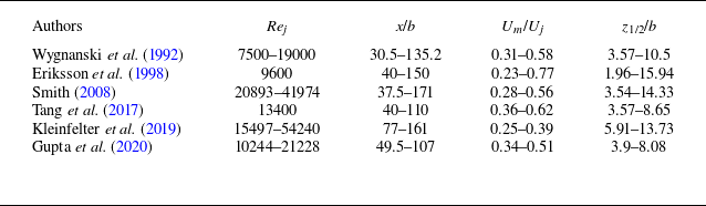
The selected datasets in this study include wall jet measurements in both air (Wygnanski et al. Reference Wygnanski, Katz and Horev1992; Smith Reference Smith2008; Kleinfelter et al. Reference Kleinfelter, Repasky, Hari, Letica, Vishwanathan, Organski, Schwaner, Alexander and Devenport2019; Gupta et al. Reference Gupta, Choudhary, Singh, Prabhakaran and Dixit2020) and water (Eriksson et al. Reference Eriksson, Karlsson and Persson1998; Tang et al. Reference Tang, Bergstrom and Bugg2017). Table 1 provides the typical ranges of experimental parameters, including Re
j
, x/b, U
m
/U
0 and z
1/2/b, considered herein for the verification of the scaling laws. Figure 4 shows the experimental data points, plotted on the (Re
j
, x/b) plane, for each study listed in table 1. For a given Re
j
, the key jet parameters, such as U
m
, z
1/2 and
 $ \tau_{0}$
, were measured at various dimensionless streamwise distances x/b. The experimental data span broad ranges of Re
j
and x/b as 7500 ≤ Re
j
≤ 54240 and 30.5 ≤ x/b ≤ 171, respectively. The selected data were obtained as follows. The data of Wygnanski et al. (Reference Wygnanski, Katz and Horev1992) were digitised from figure 5 of their paper, while those of Eriksson et al. (Reference Eriksson, Karlsson and Persson1998) were retrieved from the ERCOFTAC ‘Classic Collection’ Database. The data of Smith (Reference Smith2008) were taken from table 3.1 of his doctoral thesis, whereas those of Tang et al. (Reference Tang, Bergstrom and Bugg2017) were digitised from figures 5, 7 and 10 of their paper. Moreover, the data of Kleinfelter et al. (Reference Kleinfelter, Repasky, Hari, Letica, Vishwanathan, Organski, Schwaner, Alexander and Devenport2019) and Gupta et al. (Reference Gupta, Choudhary, Singh, Prabhakaran and Dixit2020) were compiled from table 1 of the respective papers.
Ranges of representative parameters of experimental measurements considered in this study.

Summary of experimental datasets on the (Re j , x/b) plane.

3.3. Determination of γ
The determination of γ is a critical step for obtaining α, β and χ (see (2.32), (2.33) and (2.35)–(2.38)). However, its precise estimation is challenging. George et al. (Reference George, Abrahamsson, Eriksson, Karlsson, Löfdahl and Wosnik2000) reported that γ can be determined either directly from the data (for example, by examining the slope of the U
m
versus z
1/2) or from (2.13), provided
 $ \tau_{0}$
, U
m
, dz
1/2/dx and
 $\int _{0}^{\infty }F^{2}\mathrm{d}\eta$
are known. Using the experimental data of Karlsson et al. (Reference Karlsson, Eriksson and Persson1993a
,
Reference Karlsson, Eriksson and Perssonb
), George et al. (Reference George, Abrahamsson, Eriksson, Karlsson, Löfdahl and Wosnik2000) obtained an average value of γ = 0.056.
In this study, γ is determined from the slope of the U
m
versus z
1/2 data plots. For this purpose, the entire datasets are presented in figure 5(a), plotting the dimensionless jet velocity U
m
 $v$
/M
0 as a function of dimensionless jet half-width z
1/2
M
0/
 $v$
2 on logarithmic scales. A linear regression analysis could theoretically provide the slope of the best-fit line for these data points. However, this procedure may introduce considerable error. To ensure consistency with the momentum constraint (2.13), the slope of the U
m
 $v$
/M
0 versus z
1/2
M
0/
 $v$
2 data plots (that is, −α/β ) must be less than −0.5 or, equivalently, α/β must be larger than 0.5. Small scatter in the experimental data can easily disrupt this constraint, yielding unrealistic slope estimation. Indeed, when applying the linear regression across all data points in figure 5(a), α/β was found to be less than 0.5, which is inconsistent with the theoretical expectation. Moreover, the experimental data suggest that α/β may be slightly sensitive to Re
j
. Since α/β = 0.5 represents the asymptotic limit for infinite Reynolds number, a refined approach is adopted here to accurately determine α/β for finite yet sufficiently large Re
j
. This is explained as follows.
(a) Value of U
m
 $v$
/M
0 versus z
1/2
M
0/
 $v$
2. (b) Relative error in U
m
 $v$
/M
0 versus z
1/2
M
0/
 $v$
2.

For each dataset listed in table 1, the maximum available Re
j
in the corresponding experimental facility is considered and subsequently, α/β is determined for a given Re
j
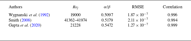
using the linear regression, verifying that the condition α/β > 0.5 is preserved. Table 2 presents the resulting values of α/β, considering the datasets of Wygnanski et al. (Reference Wygnanski, Katz and Horev1992), Smith (Reference Smith2008) and Gupta et al. (Reference Gupta, Choudhary, Singh, Prabhakaran and Dixit2020). In this regard, the dataset of Eriksson et al. (Reference Eriksson, Karlsson and Persson1998) is omitted due to relatively low Re
j
(Re
j
= 9600). For Smith (Reference Smith2008), α/β could not be precisely determined at specific values of Re
j
due to limited data points along various streamwise distances for a given Re
j
. Therefore, the data points are grouped over the maximum Re
j
range to determine α/β (table 2). However, regression analysis of the data of Tang et al. (Reference Tang, Bergstrom and Bugg2017) produced a relatively large value of α/β ≈ 0.62, whereas that of the data of Kleinfelter et al. (Reference Kleinfelter, Repasky, Hari, Letica, Vishwanathan, Organski, Schwaner, Alexander and Devenport2019) was found to consistently produce α/β < 0.5 for each value of Re
j
. The condition α/β < 0.5 in the context of the similarity solution (see § 2.2) implies a negative wall shear stress, which is impractical. Hence, table 2 also excludes the datasets of Tang et al. (Reference Tang, Bergstrom and Bugg2017) and Kleinfelter et al. (Reference Kleinfelter, Repasky, Hari, Letica, Vishwanathan, Organski, Schwaner, Alexander and Devenport2019) while estimating the value of γ. The values of the RMSE and correlation coefficient in table 2 confirm good agreement between the predicted and experimentally observed values. Finally, averaging the obtained values of α/β across the datasets results in α/β ≈ 0.525, implying γ = 0.05. This estimation is in agreement with previously reported values, such as γ = 0.056 (George et al. Reference George, Abrahamsson, Eriksson, Karlsson, Löfdahl and Wosnik2000) and 0.048 (Tang et al. Reference Tang, Rostamy, Bergstrom, Bugg and Sumner2015), although it underpredicts the value of γ = 0.084 reported by Naqavi et al. (Reference Naqavi, Tyacke and Tucker2018), due to the comparatively low Re
j
(Re
j
= 7500) used in the DNS. The current procedure for obtaining γ may appear somewhat selective. However, it is essential to carefully choose the data corresponding to large Re
j
while simultaneously satisfying the momentum constraint (2.13), which is highly sensitive to small data scatter. Notably, with γ = 0.05, the proposed scaling laws of U
m
, z
1/2 and
 $ \tau_{0}$
show excellent agreement with the experimental data (see §§ 3.6 and 3.7).
Determination of α/β.

Note that, in figure 5(a), the slope of the data plots of U
m
 $v$
/M
0 versus z
1/2
M
0/
 $v$
2 remains essentially constant, without showing any clear transition. This suggests that U
m
evolves with z
1/2 preserving a constant slope, consistent with the determination of γ for sufficiently large (though not infinite) Reynolds numbers (George et al. Reference George, Abrahamsson, Eriksson, Karlsson, Löfdahl and Wosnik2000). Therefore, the relationship between U
m
 $v$
/M
0 and z
1/2
M
0/
 $v$
2 retains a constant power-law exponent, while it is shown later that U
m
 $v$
/M
0, z
1/2
M
0/
 $v$
2 and
 $ \tau_{0}$
 $v$
2/(ρ
 $M_{0}^{2}$
) exhibit power-law scaling transitions with xM
0/
 $v$
2.
Figure 5(a) shows the best-fit line with γ = 0.05 across the data points, given by U
m
 $v$
/M
0 ≈ 1.75(z
1/2
M
0/
 $v$
2)−0.525. Analysing all the data points, we obtain the RMSE = 1.36 × 10⁻⁶ and correlation coefficient = 0.9965. For the comparison, the asymptotic law corresponding to γ = 0, that is, U
m
 $v$
/M
0 = (z
1/2
M
0/
 $v$
2)−0.5, gives the RMSE = 1.5 × 10⁻⁶ and correlation coefficient = 0.9962. These results suggest that γ = 0.05 offers an excellent estimate of the coevolution of U
m
and z
1/2. Figure 5(b) presents the relative error (in percentage) in the predicted values of U
m
 $v$
/M
0 (with γ = 0.05) as a function of z
1/2
M
0/
 $v$
2 on a semi-logarithmic plot. For the majority of the data plots, the absolute relative errors remain within 10 %. However, a few data of Kleinfelter et al. (Reference Kleinfelter, Repasky, Hari, Letica, Vishwanathan, Organski, Schwaner, Alexander and Devenport2019) show absolute relative errors ranging up to approximately 14 %. Additionally, it is observed that the data of Tang et al. (Reference Tang, Bergstrom and Bugg2017) tend to slightly overestimate the theoretical prediction, indicated by the negative relative errors.
3.4. Scaling transition for Cf
The accurate prediction of C
f
depends on the precise measurement of
 $ \tau_{0}$
. However, as noted by Launder & Rodi (Reference Launder and Rodi1979), obtaining accurate measurements of
 $ \tau_{0}$
in plane turbulent wall jets has been challenging. Several direct and indirect techniques are available for estimating
 $ \tau_{0}$
, including the use of impact tube devices such as a Stanton or Preston tube (Bradshaw & Gee Reference Bradshaw and Gee1962), the oil film interferometry (OFI) technique (Gupta et al. Reference Gupta, Choudhary, Singh, Prabhakaran and Dixit2020), evaluation from the mean velocity gradient in the viscous sublayer (Tailland & Mathieu Reference Tailland and Mathieu1967; Wygnanski et al. Reference Wygnanski, Katz and Horev1992; Eriksson et al. Reference Eriksson, Karlsson and Persson1998), the momentum integral method (Wygnanski et al. Reference Wygnanski, Katz and Horev1992), the overlap region solution (George et al. Reference George, Abrahamsson, Eriksson, Karlsson, Löfdahl and Wosnik2000) and the Clauser fit method (Tang et al. Reference Tang, Bergstrom and Bugg2017; Kleinfelter et al. Reference Kleinfelter, Repasky, Hari, Letica, Vishwanathan, Organski, Schwaner, Alexander and Devenport2019).
Figure 6 shows the comparison of the predicted scaling laws of the skin-friction coefficient C
f
with the experimental data. The data are presented plotting C
f
as a function of Re
m
on logarithmic scales. The data plots for Re
m
< 8000 respect the ‘−1/4’ power law as predicted by (2.24). However, for Re
m
> 10 000, the data plots closely follow the ‘−2/13’ power law, consistent with (2.26). A distinct scaling transition from
 ${\textit{Re}}_{m}^{-1/4}$
to
 ${\textit{Re}}_{m}^{-2/13}$
is particularly observed in the range 8000 < Re
m
< 10 000, highlighted by the shaded grey region (figure 6). This scaling transition is a manifestation of the shift in the near-wall dynamics from the buffer layer at small Re
m
to the overlap region for large Re
m
. The best-fit lines for the two scaling regions provide multiplicative constants of 0.06 and 0.024, respectively. This leads to
 \begin{equation} C_{\!f}\left({\textit{Re}}_{m}\lt 8000\right)=0.06{\textit{Re}}_{m}^{-1/4} ,\end{equation}
with the RMSE = 2.82 × 10⁻⁴ and correlation coefficient = 0.9, and
 \begin{equation} C_{\!f}\left({\textit{Re}}_{m}\gt 10\,000\right)=0.024{\textit{Re}}_{m}^{-2/13} ,\end{equation}
with the RMSE = 4.32 × 10⁻⁵ and correlation coefficient = 0.999. Additionally, for each scaling region, the error band is shown to quantify deviations between the predicted scaling law and the experimental data. For Re m < 8000 and Re m > 10 000, the majority of the data plots fall within ±5 % and ±2 % error bands, respectively, confirming an excellent agreement between theoretical predictions and experimental observations.
Comparison of the predicted scaling laws of skin-friction coefficient C f with the experimental data.

Wygnanski et al. (Reference Wygnanski, Katz and Horev1992) measured the velocity using a hot-wire sensor and determined
 $ \tau_{0}$
using a Preston tube, as well as applying the momentum integral method and the mean velocity gradient in the viscous sublayer. They argued that the latter approach provides accurate estimations. However, the estimation of
 $ \tau_{0}$
from the mean velocity gradient in the viscous sublayer was found to produce reliable results only when non-thermal measurement techniques, such as the LDV, are used (Eriksson et al. Reference Eriksson, Karlsson and Persson1998). When using hot-wire data, this technique tends to underestimate
 $ \tau_{0}$
by approximately 20 %–35 % compared with concensus values from impact tube measurements (Tailland & Mathieu Reference Tailland and Mathieu1967). As mentioned in § 3.1, the
 $ \tau_{0}$
data of Wygnanski et al. (Reference Wygnanski, Katz and Horev1992) are thus prone to errors, providing substantial underestimation of the theoretically predicted skin friction. For example, the underestimation is almost 30 % at Re
m
≈ 4000 and increases to 45 % at Re
m
≈ 7000.
Notably, the use of an impact tube assumes a universal velocity profile across the wall-normal span of the device and requires prior calibration in fully developed channel flow or zero pressure gradient TBL flow (Bradshaw & Gee Reference Bradshaw and Gee1962). Moreover, in wall jets, the location of the viscous sublayer is observed at z
+ = 3 (see figure 1
b), which is slightly different from z
+ = 5 as found in channel and TBL flows. As a consequence, both the techniques (mean velocity gradient in the viscous sublayer and impact tube devices) require appropriate corrections to the measured values of
 $ \tau_{0}$
(Gupta et al. Reference Gupta, Choudhary, Singh, Prabhakaran and Dixit2020).
Eriksson et al. (Reference Eriksson, Karlsson and Persson1998) measured the velocity using the LDV and determined
 $ \tau_{0}$
from the mean velocity gradient in the viscous sublayer. However, their experimental set-up exhibited reverse flow. The C
f
data of Eriksson et al. (Reference Eriksson, Karlsson and Persson1998) do not specifically correspond to the the ‘−1/4’ power law (figure 6). Moreover, for Re
m
< 4000, the data fall below the theoretical prediction, whereas for Re
m
> 5000, they slightly underestimate the theoretical prediction by approximately 3 %.
Tang et al. (Reference Tang, Bergstrom and Bugg2017) used the PIV data to determine
 $ \tau_{0}$
by fitting the time-averaged velocity data to the logarithmic law. Kleinfelter et al. (Reference Kleinfelter, Repasky, Hari, Letica, Vishwanathan, Organski, Schwaner, Alexander and Devenport2019) captured the wall jet using a two-dimensional, two-component time-resolved PIV. They determined
 $ \tau_{0}$
through a power-law curve fitting method. For Re
m
< 8000, both the C
f
data of Tang et al. (Reference Tang, Bergstrom and Bugg2017) and Kleinfelter et al. (Reference Kleinfelter, Repasky, Hari, Letica, Vishwanathan, Organski, Schwaner, Alexander and Devenport2019) respect the ‘−1/4’ power law, although they tend to underestimate the theoretical prediction by approximately 5 % (figure 6).
Gupta et al. (Reference Gupta, Choudhary, Singh, Prabhakaran and Dixit2020) directly measured
 $ \tau_{0}$
using the OFI technique. In this technique, a small drop of silicone fluid placed on a glass disc spreads into a thinning film, with the thinning rate proportional to
 $ \tau_{0}$
. When illuminated with near-monochromatic light, interference patterns form due to reflections from film interfaces. Then,
 $ \tau_{0}$
is linked to the rate of change of the inter-fringe spacing in the interference pattern. Gupta et al. (Reference Gupta, Choudhary, Singh, Prabhakaran and Dixit2020) emphasised that the OFI technique offers an accurate and reliable estimate of
 $ \tau_{0}$
, effectively avoiding the common limitations of traditional techniques. The C
f
data of Gupta et al. (Reference Gupta, Choudhary, Singh, Prabhakaran and Dixit2020) for Re
m
< 8000 show excellent correspondence with the ‘−1/4’ power law, subject to the ±5 % error band (figure 6), aligning well with the theoretical prediction. Moreover, for Re
m
> 10 000, the C
f
data of Kleinfelter et al. (Reference Kleinfelter, Repasky, Hari, Letica, Vishwanathan, Organski, Schwaner, Alexander and Devenport2019) support the ‘−2/13’ power law, showing a marginal deviation of ±2 % from the theoretical prediction.
Several empirical power-law relations have been previously proposed for the skin-friction coefficient, for instance C
f
= 0.0565
 ${\textit{Re}}_{m}^{-1/4}$
(Sigalla Reference Sigalla1958), C
f
= 0.0315
 ${\textit{Re}}_{m}^{-0.182}$
(Bradshaw & Gee Reference Bradshaw and Gee1962), C
f
= 0.0667
 ${\textit{Re}}_{m}^{-0.258}$
(Hammond Reference Hammond1982) and C
f
= 0.0179
 ${\textit{Re}}_{m}^{-0.113}$
(Eriksson et al. Reference Eriksson, Karlsson and Persson1998). Strikingly, the empirical relation of Sigalla (Reference Sigalla1958) closely resembles (3.1).
The scaling laws of C
f
with Re
m
can also be expressed as a function of xM
0/
 $v$
2, because both U
m
and z
1/2 vary with the streamwise distance. Since z
m
∼ z
1/2, substituting (1.4) and (1.5) into (3.1) and then using (2.32) and (2.33) yields C
f
(Re
m
< 8000) ∼ (xM
0/
 $v$
2)−(1−γ)/(9−γ). Similarly, substituting (1.4) and (1.5) into (3.2) and then using (2.35) and (2.36) leads to C
f
(Re
m
> 10 000) ∼ (xM
0/
 $v$
2)−(1−γ)/(14−γ). Applying γ = 0.05 results in C
f
(Re
m
< 8000) ∼ (xM
0/
 $v$
2)−0.1061 and C
f
(Re
m
> 10 000) ∼ (xM
0/
 $v$
2)−0.0681.
3.5. Discussion on Cf in wall jets
It is important to emphasise that one must exercise caution when drawing conclusions about C
f
in wall jets, because of the lack of a generic consensus on how to determine
 $ \tau_{0}$
. For instance, the ‘−2/13’ power-law region in figure 6 contains only the data of Kleinfelter et al. (Reference Kleinfelter, Repasky, Hari, Letica, Vishwanathan, Organski, Schwaner, Alexander and Devenport2019), who obtained
 $ \tau_{0}$
using the Clauser fit method. Although details of their fitting procedure were not described explicitly, this method generally involves fitting the near-wall velocity data to the conventional logarithmic law. However, the validity of the logarithmic law in wall jets remains dubious. This raises a question: How reliable is the Clauser fit method in wall jets, given that no standard procedure exists for determining
 $ \tau_{0}$
based on a universally accepted near-wall velocity profile? If its reliability is uncertain, then how can the data of Kleinfelter et al. (Reference Kleinfelter, Repasky, Hari, Letica, Vishwanathan, Organski, Schwaner, Alexander and Devenport2019) for Re
m
> 10 000 justify the existence of the ‘−2/13’ power law? These critical issues are discussed below.
The logarithmic law for the overlap region in canonical flows is expressed as u
+ = (1/κ)ln z
+ + B, where u
+ =
 $\overline{u}$
/u
*, κ = 0.41 is the von Kármán constant and B = 5 is the intercept. The experimental studies of Eriksson et al. (Reference Eriksson, Karlsson and Persson1998) and Tang et al. (Reference Tang, Bergstrom and Bugg2017), together with the DNS of Naqavi et al. (Reference Naqavi, Tyacke and Tucker2018), provide evidence for the validity of the logarithmic law in wall jets, lending credibility to the Clauser fit as a potential method to determine C
f
. However, the universality of the logarithmic-law coefficients, such as κ and B, remains debated. For example, Banyassady & Piomelli (Reference Banyassady and Piomelli2015) compiled various estimates of κ and B in the ranges κ = 0.41−0.6 and B = 5−9.5. Despite this variability, figure 6 shows that, for Re
m
< 8000, the C
f
data obtained using the Clauser fit method (Tang et al. Reference Tang, Bergstrom and Bugg2017; Kleinfelter et al. Reference Kleinfelter, Repasky, Hari, Letica, Vishwanathan, Organski, Schwaner, Alexander and Devenport2019) are consistent (subject to ±5 % error band) with those obtained from the OFI technique (Gupta et al. Reference Gupta, Choudhary, Singh, Prabhakaran and Dixit2020) and from the mean velocity gradient in the viscous sublayer (Eriksson et al. Reference Eriksson, Karlsson and Persson1998). This agreement provides confidence in extending the Clauser fit based estimates to sufficiently large Re
m
(Re
m
> 10 000).
For Re
m
> 10 000, however, the C
f
data of Kleinfelter et al. (Reference Kleinfelter, Repasky, Hari, Letica, Vishwanathan, Organski, Schwaner, Alexander and Devenport2019) exhibit a slight deviation from the ‘−2/13’ power law (figure 6). A regression analysis of the data yields a slope of −0.182. This value is somewhat steeper than the theoretical prediction of −2/13 (≈ −0.154), although the data plots remain within the ±2 % error band. Importantly, when the ‘−2/13’ power law of C
f
is applied, the predicted scaling laws of U
m
and z
1/2 for Re
m
> 10 000 show remarkable agreement with the data (see § 3.6). This agreement is particularly compelling because the experimental measurements of U
m
and z
1/2 are relatively straightforward and involve far less uncertainty than the determination of
 $ \tau_{0}$
. This reinforces the consistency of the ‘−2/13’ power law of C
f
. Accordingly, the modest deviation of the C
f
data of Kleinfelter et al. (Reference Kleinfelter, Repasky, Hari, Letica, Vishwanathan, Organski, Schwaner, Alexander and Devenport2019) from the ‘−2/13’ power law is interpreted as a consequence of methodological uncertainties inherent in the Clauser fit, rather than as evidence of any inconsistency in the predicted scaling law.
Similar reasoning can be applied to explain why the C
f
data of Kleinfelter et al. (Reference Kleinfelter, Repasky, Hari, Letica, Vishwanathan, Organski, Schwaner, Alexander and Devenport2019) show no clear evidence of a scaling transition from Re
m
< 8000 to Re
m
> 10 000, instead exhibiting a constant slope of −0.182 across the entire range of Re
m
(figure 6). This apparent discrepancy can reasonably be attributed to uncertainties in the exact methodology employed to determine C
f
. Nevertheless, the scaling transition for C
f
from Re
m
< 8000 to Re
m
> 10 000 is inevitable, because incorporating this transition into the mathematical framework yields corresponding transitions in U
m
and z
1/2, both of which show excellent agreement with the data (see § 3.6). Therefore, the power-law scaling transition for C
f
in wall jets holds true. However, accurate measurements of
 $ \tau_{0}$
in wall jets are essential to provide stronger experimental support for this transition.
(a) Comparison of the predicted scaling laws of dimensionless jet velocity U
m
 $v$
/M
0 with the experimental data. (b) Plot of U
m
 $v$
/M
0 versus xM
0/
 $v$
2 along with the experimental data grouped into three categories of Re
m
.

3.6. Scaling transitions for Um and z 1/2
The scaling transition for U
m
is presented in figure 7. Figure 7(a) compares the predicted scaling laws of the dimensionless jet velocity U
m
 $v$
/M
0 with the experimental data. The data are presented by plotting U
m
 $v$
/M
0 as a function of xM
0/
 $v$
2 on logarithmic scales. To examine the influence of Re
m
, figure 7(b) groups the data points from figure 7(a) into three distinct ranges: Re
m
< 8000, 8000 < Re
m
< 10 000 and Re
m
> 10 000. The data plots show reasonably good collapse on the plane formed by U
m
 $v$
/M
0 and xM
0/
 $v$
2. It is found that, for Re
m
< 8000, the data extend up to xM
0/
 $v$
2 = 4.92 × 10¹⁰, whereas for Re
m
> 10 000, they begin from xM
0/
 $v$
2 = 5.37 × 10¹⁰. For xM
0/
 $v$
2 ≤ 4.92 × 10¹⁰, the data plots respect the ‘−4(1 + γ)/(9 − γ)’ power law (see (2.32)), whereas for xM
0/
 $v$
2 ≥ 5.37 × 10¹⁰, they follow the ‘−13(1 + γ)/[2(14 − γ)]’ power law (see (2.35)). This confirms that the scaling transition occurs with increasing xM
0/
 $v$
2, typically within the range 4.92 × 10¹⁰ < xM
0/
 $v$
2 < 5.37 × 10¹⁰. With γ = 0.05, the best-fit lines across the data points (excluding those for 8000 < Re
m
< 10 000) yield
 \begin{equation} \frac{U_{m}v }{M_{0}}\left(\frac{{\textit{xM}}_{0}}{v ^{2}}\leq 4.92\times 10^{10}\right)=1.7\left(\frac{{\textit{xM}}_{0}}{v ^{2}}\right)^{-0.4693} ,\end{equation}
with the RMSE = 2 × 10⁻⁶ and correlation coefficient = 0.986, and
 \begin{equation} \frac{U_{m}v }{M_{0}}\left(\frac{{\textit{xM}}_{0}}{v ^{2}}\geq 5.37\times 10^{10}\right)=2.6\left(\frac{{\textit{xM}}_{0}}{v ^{2}}\right)^{-0.4892} ,\end{equation}
with the RMSE = 1.9 × 10− 7 and correlation coefficient = 0.997.
Most of the data plots for both scaling regions fall within the ±10 % and ±5 % error bands, corresponding to xM
0/
 $v$
2 ≤ 4.92 × 10¹⁰ and xM
0/
 $v$
2 ≥ 5.37 × 10¹⁰, respectively. This indicates satisfactory agreement between theoretical predictions and experimental observations (figure 7
a,b). For Re
m
< 8000 (or xM
0/
 $v$
2 ≤ 4.92 × 10¹⁰), a few U
m
data of Kleinfelter et al. (Reference Kleinfelter, Repasky, Hari, Letica, Vishwanathan, Organski, Schwaner, Alexander and Devenport2019) tend to underestimate the theoretical prediction by approximately 12 %, whereas those of Tang et al. (Reference Tang, Bergstrom and Bugg2017) overestimate it by approximately 13 % (figure 7
a). Overall, the U
m
data of Wygnanski et al. (Reference Wygnanski, Katz and Horev1992), Eriksson et al. (Reference Eriksson, Karlsson and Persson1998) and Gupta et al. (Reference Gupta, Choudhary, Singh, Prabhakaran and Dixit2020) have an excellent match with the theoretical prediction, subject to the ±10 % error band. On the other hand, for Re
m
> 10 000 (or xM
0/
 $v$
2 ≥ 5.37 × 10¹⁰), the U
m
data of Smith (Reference Smith2008) and Kleinfelter et al. (Reference Kleinfelter, Repasky, Hari, Letica, Vishwanathan, Organski, Schwaner, Alexander and Devenport2019) corroborate the theoretical prediction within the ±5 % error band. It is worth mentioning that, for 8000 < Re
m
< 10 000, (3.3) and (3.4) are not strictly valid. This is due to the fact that the exponents in (3.3) and (3.4) lose their validity in the range 8000 < Re
m
< 10 000, as C
f
in this range undergoes a transition without adhering to a well-defined power law (see figure 6). Nevertheless, figure 7(b) shows that for 8000 < Re
m
< 10 000, (3.3) and (3.4) still provide reasonable approximations, because (3.3) aligns with the data for xM
0/
 $v$
2 ≤ 4.92 × 10¹⁰, whereas (3.4) captures the data for xM
0/
 $v$
2 ≥ 5.37 × 10¹⁰. Additionally, it is observed that for 4.92 × 10¹⁰ < xM
0/
 $v$
2 < 5.37 × 10¹⁰, either (3.3) or (3.4) is capable of capturing the data belonging to 8000 < Re
m
< 10 000.
(a) Comparison of the predicted scaling laws of dimensionless jet half-width z
1/2
M
0/
 $v$
2 with the experimental data. (b) Plot of z
1/2
M
0/
 $v$
2 versus xM
0/
 $v$
2 along with the experimental data grouped into three categories of Re
m
.

The scaling transition for z
1/2 is presented in figure 8. Figure 8(a) shows the comparison of the predicted scaling laws of the dimensionless jet half-width z
1/2
M
0/
 $v$
2 with the experimental data. The data are presented plotting z
1/2
M
0/
 $v$
2 as a function of xM
0/
 $v$
2 on logarithmic scales. To further explore the impact of Re
m
, figure 8(b) groups the data points from figure 8(a) into three different ranges: Re
m
< 8000, 8000 < Re
m
< 10 000 and Re
m
> 10 000. A satisfactory collapse of the data plots is observed on the plane formed by z
1/2
M
0/
 $v$
2 and xM
0/
 $v$
2. For Re
m
< 8000, the data are observed up to xM
0/
 $v$
2 = 4.92 × 10¹⁰, while for Re
m
> 10 000, they begin from xM
0/
 $v$
2 = 5.37 × 10¹⁰. For xM
0/
 $v$
2 ≤ 4.92 × 10¹⁰, the data plots follow the ‘8/(9 − γ)’ power law as described by (2.33). Conversely, for xM
0/
 $v$
2 ≥ 5.37 × 10¹⁰, the data plots obey the ‘13/(14 − γ)’ power law as given by (2.36). The scaling transition takes place in the range 4.92 × 10¹⁰ < xM
0/
 $v$
2 < 5.37 × 10¹⁰. With γ = 0.05, the best-fit lines across the data points (excluding those for 8000 < Re
m
< 10 000) yield
 \begin{equation} \frac{z_{1/2}M_{0}}{v ^{2}}\left(\frac{{\textit{xM}}_{0}}{v ^{2}}\leq 4.92\times 10^{10}\right)=1.06\left(\frac{{\textit{xM}}_{0}}{v ^{2}}\right)^{0.8939} ,\end{equation}
with the RMSE = 1.23 × 10⁸ and correlation coefficient = 0.993, and
 \begin{equation} \frac{z_{1/2}M_{0}}{v ^{2}}\left(\frac{{\textit{xM}}_{0}}{v ^{2}}\geq 5.37\times 10^{10}\right)=0.475\left(\frac{{\textit{xM}}_{0}}{v ^{2}}\right)^{0.9319} ,\end{equation}
with the RMSE = 5.58 × 10⁸ and correlation coefficient = 0.998.
Compensated plots of the scaling laws of (a) U
m
 $v$
/M
0 and (b) z
1/2
M
0/
 $v$
2.

The theoretical predictions are in good agreement with the experimental data, as most data plots for both scaling regions are confined to the ±10 % error band (figure 8
a,b). For Re
m
< 8000 (or xM
0/
 $v$
2 ≤ 4.92 × 10¹⁰), the z
1/2 data of Eriksson et al. (Reference Eriksson, Karlsson and Persson1998) and Tang et al. (Reference Tang, Bergstrom and Bugg2017) tend to underestimate the theoretical prediction by nearly ±10 %, whereas a few z
1/2 data of Gupta et al. (Reference Gupta, Choudhary, Singh, Prabhakaran and Dixit2020) underestimate it by approximately 18 %. The z
1/2 data of Wygnanski et al. (Reference Wygnanski, Katz and Horev1992) and Kleinfelter et al. (Reference Kleinfelter, Repasky, Hari, Letica, Vishwanathan, Organski, Schwaner, Alexander and Devenport2019) show satisfactory agreement with the theoretical prediction, subject to the ±10 % error band (figure 8
a). For Re
m
> 10 000 (or xM
0/
 $v$
2 ≥ 5.37 × 10¹⁰), the z
1/2 data of Smith (Reference Smith2008) and Kleinfelter et al. (Reference Kleinfelter, Repasky, Hari, Letica, Vishwanathan, Organski, Schwaner, Alexander and Devenport2019) align well with the theoretical prediction as the data plots fall within the ±10 % error band. Although (3.5) and (3.6) do not strictly apply for 8000 < Re
m
< 10 000, they offer reasonable approximations for capturing the data corresponding to this range (figure 8
b). Specifically, (3.5) captures the data for xM
0/
 $v$
2 ≤ 4.92 × 10¹⁰, whereas (3.6) performs well for xM
0/
 $v$
2 ≥ 5.37 × 10¹⁰. For 4.92 × 10¹⁰ < xM
0/
 $v$
2 < 5.37 × 10¹⁰, either (3.5) or (3.6) satisfactorily captures the data corresponding to 8000 < Re
m
< 10 000.
To better illustrate the scaling transitions for U
m
and z
1/2, figure 9 shows compensated plots of both U
m
 $v$
/M
0 and z
1/2
M
0/
 $v$
2 along with the experimental data grouped into three ranges of Re
m
. In figure 9
a, the data are presented plotting (U
m
 $v$
/M
0)(xM
0/
 $v$
2)0.4693 as a function of xM
0/
 $v$
2 on semilogarithmic scales, along with (3.3) and (3.4). Similarly, in figure 9
b, the data are presented plotting (z
1/2
M
0/
 $v$
2)(xM
0/
 $v$
2)−0.8939 as a function of xM
0/
 $v$
2, together with (3.5) and (3.6). The emergence of plateaus in figure 9(a,b) confirms the validity of the scaling laws (3.3) and (3.5) for Re
m
< 8000 (or xM
0/
 $v$
2 ≤ 4.92 × 10¹⁰). The systematic departure of data from the plateaus with increasing Re
m
indicates a scaling transition, thereby supporting the applicability of (3.4) and (3.6) for Re
m
> 10 000 (or xM
0/
 $v$
2 ≥ 5.37 × 10¹⁰).
(a) Comparison of the predicted scaling laws of dimensionless wall shear stress
 $ \tau_{0}$
 $v$
2/(ρ
 $M_{0}^{2}$
) with the experimental data. (b) Plot of
 $ \tau_{0}$
 $v$
2/(ρ
 $M_{0}^{2}$
) versus xM
0/
 $v$
2 along with the experimental data grouped into three categories of Re
m
.

3.7. Scaling transition for
$ \tau_{0}$

The scaling transition for
 $ \tau_{0}$
is presented in figure 10. Figure 10(a) compares the predicted scaling laws of the dimensionless wall shear stress
 $ \tau_{0}$
 $v$
2/(ρ
 $M_{0}^{2}$
) with the experimental data. The data are presented plotting
 $ \tau_{0}$
 $v$
2/(ρ
 $M_{0}^{2}$
) as a function of xM
0/
 $v$
2 on logarithmic scales. Furthermore, figure 10(b) shows the influence of Re
m
, grouping the data points from figure 10(a) into three distinct ranges: Re
m
< 8000, 8000 < Re
m
< 10 000 and Re
m
> 10 000. A reasonable collapse of the data plots is found on the plane formed by
 $ \tau_{0}$
 $v$
2/(ρ
 $M_{0}^{2}$
) and xM
0/
 $v$
2. For Re
m
< 8000, the data span up to xM
0/
 $v$
2 = 4.92 × 10¹⁰, whereas for Re
m
> 10 000, they commence from xM
0/
 $v$
2 = 7.4 × 10¹⁰. For xM
0/
 $v$
2 ≤ 4.92 × 10¹⁰, the data plots follow the ‘−(9 + 7γ)/(9 − γ)’ power law as predicted by (2.37). By contrast, for xM
0/
 $v$
2 ≥ 7.4 × 10¹⁰, the data plots follow the ‘−(14 + 12γ)/(14 − γ)’ power law, consistent with (2.38). The scaling transition occurs in the range 4.92 × 10¹⁰ < xM
0/
 $v$
2 < 7.4 × 10¹⁰. Notably, this range appears wider than the corresponding transition range for U
m
and z
1/2, that is, 4.92 × 10¹⁰ < xM
0/
 $v$
2 < 5.37 × 10¹⁰ (see figures 7 and 8). This is because the dataset of Smith (Reference Smith2008) lacked measurements of
 $ \tau_{0}$
, as mentioned in § 3.1. It is not appropriate to determine the numerical coefficients in the
 $ \tau_{0}$
 $v$
2/(ρ
 $M_{0}^{2}$
) versus xM
0/
 $v$
2 scaling relationship solely through the regression analysis. To ensure consistency between the wall shear stress prediction and the skin-friction laws (see (3.1) and (3.2)), the numerical coefficient for Re
m
< 8000 is derived by combining (3.1), (3.3) and (3.5), whereas that for Re
m
> 10 000 is obtained using (3.2), (3.4) and (3.6). In this process, an average value of z
m
/z
1/2 is considered as 0.15 (Wygnanski et al. Reference Wygnanski, Katz and Horev1992; Gupta et al. Reference Gupta, Choudhary, Singh, Prabhakaran and Dixit2020; Choudhary et al. Reference Choudhary, Gupta, Bhatt, Prabhakaran, Singh, Karipot and Dixit2024). With γ = 0.05, the resulting expressions for
 $ \tau_{0}$
are as follows:
 \begin{align} \frac{\tau _{0}v ^{2}}{\rho M_{0}^{2}}\left(\frac{{\textit{xM}}_{0}}{v ^{2}}\leq 4.92\times 10^{10}\right)&=0.12\left(\frac{{\textit{xM}}_{0}}{v ^{2}}\right)^{-1.0447} , \end{align}
 \begin{align} \frac{\tau _{0}v ^{2}}{\rho M_{0}^{2}}\left(\frac{{\textit{xM}}_{0}}{v ^{2}}\geq 7.4\times 10^{10}\right)&=0.105\left(\frac{{\textit{xM}}_{0}}{v ^{2}}\right)^{-1.0466} . \end{align}
For Re
m
< 8000 (or xM
0/
 $v$
2 ≤ 4.92 × 10¹⁰), the theoretical prediction (3.7) satisfactorily captures the experimental data of Eriksson et al. (Reference Eriksson, Karlsson and Persson1998), Tang et al. (Reference Tang, Bergstrom and Bugg2017), Kleinfelter et al. (Reference Kleinfelter, Repasky, Hari, Letica, Vishwanathan, Organski, Schwaner, Alexander and Devenport2019) and Gupta et al. (Reference Gupta, Choudhary, Singh, Prabhakaran and Dixit2020), subject to the ±20 % error band (figure 10
a,b). For Re
m
< 8000, all the datasets produce the RMSE = 4.39 × 10−
13 and correlation coefficient = 0.995. For Re
m
> 10 000 (or xM
0/
 $v$
2 ≥ 7.4 × 10¹⁰), the theoretical prediction (3.8) closely aligns with the experimental data of Kleinfelter et al. (Reference Kleinfelter, Repasky, Hari, Letica, Vishwanathan, Organski, Schwaner, Alexander and Devenport2019), subject to ±10 % error band (figure 10
a), with the RMSE = 6.51 × 10⁻¹⁵ and correlation coefficient = 0.998.
It is also essential to verify whether the numerical coefficients in (3.7) and (3.8) are consistent with the momentum integral relation (2.12). In (2.12), the integral term
 $\int _{0}^{\infty }F^{2}\mathrm{d}\eta$
can be determined either theoretically by assigning a functional form for the self-similar velocity profile F(η) or experimentally through numerical integration of the square of the measured self-similar velocity data. The experimental study of Wygnanski et al. (Reference Wygnanski, Katz and Horev1992) and more recent measurements by Gupta et al. (Reference Gupta, Choudhary, Singh, Prabhakaran and Dixit2020) provided an average value of the integral term as 0.74. Therefore, utilising
 $\int _{0}^{\infty }F^{2}\mathrm{d}\eta$
= 0.74 and substituting (3.3) and (3.5) into (2.12) produces
 $ \tau_{0}$
 $v$
2/(ρ
 $M_{0}^{2}$
) = 0.1(xM
0/
 $v$
2)−1.0447, which shows a close agreement with (3.7). Similarly, substituting (3.4) and (3.6) into (2.12) yields
 $ \tau_{0}$
 $v$
2/(ρ
 $M_{0}^{2}$
) = 0.11(xM
0/
 $v$
2)−1.0466, which closely matches (3.8).
3.8. Comparison of scaling exponents with previous studies
Table 3 presents a comparison of the scaling exponents α, β and χ obtained from this study with those reported in earlier studies (Narasimha et al. Reference Narasimha, Narayan and Parthasarathy1973; Wygnanski et al. Reference Wygnanski, Katz and Horev1992; Barenblatt et al. Reference Barenblatt, Chorin and Prostokishin2005; Smith Reference Smith2008; Rostamy et al. Reference Rostamy, Bergstrom, Sumner and Bugg2011a
; Tang et al. Reference Tang, Rostamy, Bergstrom, Bugg and Sumner2015, Reference Tang, Bergstrom and Bugg2017; Naqavi et al. Reference Naqavi, Tyacke and Tucker2018; Kleinfelter et al. Reference Kleinfelter, Repasky, Hari, Letica, Vishwanathan, Organski, Schwaner, Alexander and Devenport2019). While all previous studies reported single values for α, β and χ, this study reveals that each scaling exponent undergoes a transition. For U
m
 $v$
/M
0, the transition of α from 0.4693 to 0.4892 corresponds to an increase of approximately 4.2 %. Similarly, for z
1/2
M
0/
 $v$
2, the transition of β from 0.8939 to 0.9319 indicates an increase of nearly 4.3 %. For
 $ \tau_{0}$
 $v$
2/(ρ
 $M_{0}^{2}$
), the transition of χ from 1.0447 to 1.0466 shows a smaller increase of approximately 0.2 %. At first glance, these changes might appear to fall within the data uncertainty band, since the data scatter is generally at least ±5 %. However, the differences become statistically significant for large xM
0/
 $v$
2. For example, if (3.3) is extrapolated up to xM
0/
 $v$
2 = 4 × 10¹¹, it overpredicts U
m
 $v$
/M
0 relative to (3.4) by 11.3 %, thus lying outside the ±5 % error band shown in figure 7. Similarly, (3.5) for xM
0/
 $v$
2 = 4 × 10¹¹ underpredicts z
1/2
M
0/
 $v$
2 relative to (3.6) by 19.1 %, exceeding the 10 % error margin (figure 8). Likewise, (3.7) for xM
0/
 $v$
2 = 4 × 10¹¹ underpredicts
 $ \tau_{0}$
 $v$
2/(ρ
 $M_{0}^{2}$
) relative to (3.8) by 20.2 %, thereby lying beyond the ±10 % error band (figure 10).
Comparison of the scaling exponents α, β and χ.

4. Conclusions
In this study, we demonstrate that, in a fully developed plane turbulent wall jet, the dimensionless jet velocity U
m
 $v$
/M
0, jet half-width z
1/2
M
0/
 $v$
2 and wall shear stress
 $ \tau_{0}$
 $v$
2/(ρ
 $M_{0}^{2}$
) exhibit distinct power-law scaling transitions with the dimensionless streamwise distance xM
0/
 $v$
2. Our theoretical framework provides a systematic approach for determining the scaling exponents α, β and χ. First, an expression for
 $ \tau_{0}$
is obtained by applying similarity scaling relationships to the governing equations. Subsequently, an independent scaling law of
 $ \tau_{0}$
is derived based on the momentum exchange caused by near-wall turbulent eddies. Equating the scaling exponents of
 $ \tau_{0}$
derived from these expressions allows us to determine α, β and χ as a function of γ, where γ ≈ 0.05 represents a key parameter governing the coevolution of jet velocity and half-width.
In the theoretical analysis,
 $ \tau_{0}$
is determined from the magnitude of the Reynolds shear stress at a near-wall reference level. The Reynolds shear stress, generated by a turbulent eddy that straddles the reference level and facilitates momentum exchange, is determined by multiplying the eddy-induced momentum contrast across this level with the eddy turnover velocity. The eddy turnover velocity is obtained by applying Kolmogorov’s two-thirds law. The TKE dissipation rate at the reference level is derived from the energy equation, which provides an approximate balance between the TKE production rate and the TKE dissipation rate. For moderate Re
m
, the reference level lies a few times above the viscous sublayer thickness. However, for sufficiently large Re
m
, it shifts to the centre of the mesolayer, where the Reynolds shear stress gradient vanishes. The results reveal that C
f
transitions from
 ${\textit{Re}}_{m}^{-1/4}$
to
 ${\textit{Re}}_{m}^{-2/13}$
(or from (xM
0/
 $v$
2)−(1−γ)/(9−γ) to (xM
0/
 $v$
2)−(1−γ)/(14−γ)) as Re
m
shifts from moderate (Re
m
< 8000) to sufficiently large (Re
m
> 10 000) values. For Re
m
< 8000, the scaling exponents are α = 4(1 + γ)/(9 − γ), β = 8/(9 − γ) and χ = (9 + 7γ)/(9 − γ), while for Re
m
> 10 000, they switch to α = 13(1 + γ)/[2(14 − γ)], β = 13/(14 − γ) and χ = (14 + 12γ)/(14 − γ). Our theoretical predictions show remarkable agreement with experimental data.
Studying scaling transitions in canonical flows is important because they indicate fundamental changes in the governing dynamics. In wall jets, this study is the first to reveal such transitions, which delineate the limits of validity of existing empirical laws for U
m
, z
1/2 and
 $ \tau_{0}$
, thus offering deeper insights into the coupling between the skin friction, jet velocity and jet half-width. The proposed scaling transitions open new avenues for improved modelling of wall jets. Nevertheless, a more detailed understanding of these transitions, especially in relation to the flow field and arrangement of turbulent eddies, remains a subject for future research.
Declaration of interests
The authors report no conflict of interest.