2.1. Simulation set-up

In this work, LES of a supersonic underexpanded planar jet is conducted with a Reynolds number based on the nozzle height of $Re_h =\rho _\infty a_\infty h/{\mu _\infty } = 1.86 \times 10^5$, where $\rho _\infty$, $a_\infty$ and $\mu _\infty$ denote the far-field density, sound velocity and molecular viscosity, respectively. The compressible LES governing equations are non-dimensionalized by the nozzle exit height ($h$) and ambient physical parameters ($\rho _\infty$, $a_\infty$, $T_\infty$, $\mu _\infty$). The lip thickness ($\delta _p$) of the jet nozzle is $h/8$. The nozzle design Mach number ($M_d$) is 1, operating under conditions with a nozzle pressure ratio (ratio of internal pressure (${p_e}$) to ambient pressure (${p_\infty }$)) of 2.09. The ideally expanded Mach number $M_j = U_j/a_j$ is 1.55, where $U_j=430.9\ {\rm m}\ {\rm s}^{-1}$ and $a_j=278\ {\rm m}\ {\rm s}^{-1}$ are velocity and sound speeds at ideally expanded conditions of the jet. The momentum thickness of the boundary layer ($\delta _\theta /h$) at the nozzle inlet is $5.0 \times 10^{-3}$. In general, the current jet parameters are very close to the previous experiment of Raman (Reference Raman1997) and numerical simulations of Berland, Bogey & Bailly (Reference Berland, Bogey and Bailly2007) and Ye et al. (Reference Ye, Zhang, Wan, Sun and Lu2020). The results obtained with the current jet parameters show good agreement with experimental and numerical simulation results, as elaborated in our previous study (Liang et al. Reference Liang, Wan, Ye, Zhang, Sun and Lu2023).

High-order finite difference methods are utilized to discretize the compressible governing equations in an in-house compressible flow solver HiResX, which has been validated in various flow systems (Li et al. Reference Li, Ye, Wan, Liu, Sun and Lu2020a; Ye et al. Reference Ye, Zhang, Wan, Sun and Lu2020, Reference Ye, Zhang, Wan, Yan and Sun2022). To capture the discontinuities caused by shock waves in the supersonic jet plume, a fifth-order alternative formulation of the weighted essentially non-oscillatory scheme (Jiang, Shu & Zhang Reference Jiang, Shu and Zhang2013) is employed for discretizing the convective fluxes. The derivatives of viscous fluxes are discretized by applying the sixth-order central difference scheme. The subgrid-scale term can be modelled by a wall-adapting local eddy viscosity model (Nicoud & Ducros Reference Nicoud and Ducros1999). The temporal advancement is performed by the three-stage total variation diminishing Runge–Kutta scheme (Shu & Osher Reference Shu and Osher1988) to ensure temporal accuracy. Additionally, all cases were computed on clusters of graphics processing units.

Figure 1 presents the schematic diagram of the computational domain and boundary conditions for numerical simulations. A relatively large computational domain is utilized, with sponge zones set up around the physical domain to prevent spurious reflections at the boundaries. The computational domain extends from $-20h$ to $80h$ in the $x$ direction, from $-25h$ to $25h$ in the $y$ direction and from $-2.5h$ to $2.5h$ in the $z$ direction. The origin of the coordinate system is fixed at the centre of the nozzle exit. The baseline case uses a structured mesh with $62.3\times 10^6$ cells to discretize the computational domain. For the control case, local mesh refinement is applied near the forcing region, resulting in a total of $64.0\times 10^6$ mesh cells. On the solid wall, no-slip adiabatic boundary conditions are used. Riemann characteristic boundary conditions are set on the outflow and transverse boundaries of the computational domain, while the periodic boundary conditions are used in the spanwise direction. Initially, the flow solver is initialized to a static flow condition. For all cases, simulations are performed for 200 dimensionless time units to ensure that turbulence is fully developed, followed by an additional 300 dimensionless time units for statistical analysis. The time step is fixed at $\Delta ta_\infty /h = 8 \times 10^{-4}$. The number of stored instantaneous full three-dimensional (3-D) flow fields is 1000 with a time interval of $0.16$. A total number of 5000 slice snapshots parallel to the $y$ direction are stored with a time interval of $0.04$, to ensure that these data have a sufficient temporal resolution for statistical analysis.

Figure 1.

Schematic diagram of computational domain and boundary conditions for numerical simulations (not to scale). (a) Computational set-up for supersonic underexpanded planar jets; (b) magnified view of nozzle; (c) unsteady forcing with the spanwise wavenumber $k_ch=2 {\rm \pi}$.

2.2. Unsteady control set-up

A periodic wall-normal momentum perturbation is introduced by implementing a periodic suction and blowing at the wall to achieve active control of jet noise. The actuator is simultaneously applied on both the upper and lower surfaces of the nozzle in the vicinity of the nozzle exit, centred at $L_a/h=-0.2$ with a width of $L_x/h=0.1$. Here $L_a$ and $L_x$ represent the centre position and streamwise length of the actuator, respectively. The actuators are in-phase. This configuration is illustrated by the red dashed line in figure 1(b). The wall-normal suction and blowing velocity profile follows previous investigations (Liu et al. Reference Liu, Sun, Yeh, Ukeiley, Cattafesta and Taira2021), which is modelled as

(2.1)\begin{equation} v_{jet}(x,z,t) = A\sin ({\omega}_at){\it \varTheta}(x,L_a,L_x) \cos (k_cz), \end{equation}

where $A$ is the forcing amplitude, $\omega _a$ and $k_c$ represent the forcing frequency and spanwise wavenumber, respectively. Here ${\it \varTheta }(x,L_a,L_x)$ is the function describing the imposed spatial velocity distribution, defined as follows:

(2.2)\begin{equation} {\it \varTheta}(x,L_a,L_x) = \tfrac{1}{4}\{1+\tanh [\eta_1(x-L_a+L_x/\eta_2)] \}\{1-\tanh [\eta_1(x-L_a-L_x/\eta_2)] \}, \end{equation}

avoiding velocity discontinuity in the streamwise direction, as shown in figure 1(c). In this study, $\eta _1=2000$ and $\eta _2=2.6$ are chosen. The suction and blowing capability of the actuator is characterized by the unsteady momentum coefficient, defined as

(2.3)\begin{equation} C_{\mu} \equiv \frac{I}{\tfrac{1}{2}{\rho_\infty}{a_\infty^2}L_zh}, \end{equation}

where $I=({\rho _w}/{T_a})\int _{0}^{T_a}\int _{-L_z/2}^{L_z/2} \int _{L_a-L_x/2}^{L_a+L_x/2}v_{jet}^2(x,z,t)\,\mathrm {d}\kern0.06em x\,\mathrm {d}z\,\mathrm {d}t$ is the time-averaged jet momentum, $\rho _w$ is the density at the wall, $T_a=2{\rm \pi} /\omega _a$ is the period of unsteady forcing. In this study, we select two momentum coefficients, $C_\mu =0.0015 (A=33.87\ {\rm m}\ {\rm s}^{-1})$ and $0.0094 (86.38\ {\rm m}\ {\rm s}^{-1})$, to validate the effectiveness of the frequency and wavenumber guided by the resolvent analysis at different amplitudes.

The noise reduction effectiveness is evaluated by the average difference in OASPL between the controlled and baseline flow fields across monitoring points distributed upstream and downstream, which is defined as

(2.4)\begin{equation} \Delta{OASPL_{avg}}=\frac{1}{N_m}\sum_{i=1}^{N_m}(OASPL_{i}^{Controlled}- OASPL_{i}^{Baseline}), \end{equation}

where $(\bullet )^{Controlled}$ and $(\bullet )^{Baseline}$, respectively, represent the variables of the controlled and baseline cases. Here $(\bullet )_{avg}$ is the average value of the variables and $N_m$ is the number of monitoring points arranged in the flow field. As shown in figure 2, the arrangement of monitoring points is relatively extensive, with those marked in green participating in the averaging. Therefore, $\Delta {OASPL_{avg}}$ is considered to be a satisfactory quantitative measure for assessing the effectiveness of noise reduction.

Figure 2.

A schematic diagram illustrating the spatial distribution of all monitoring points. The dashed lines indicate the regions of forcing and response for the acoustic resolvent analysis.

2.3. Standard and acoustic resolvent formulation

Resolvent analysis is an operator-based modal decomposition method that characterizes the input–output properties of a dynamic system and analyses the response to harmonic forcing input at a given state. The Reynolds decomposition

(2.5)\begin{equation} \boldsymbol{q}(\boldsymbol{x},t)=\bar{\boldsymbol{q}} (\boldsymbol{x})+\boldsymbol{q^{\prime}}(\boldsymbol{x},t) , \end{equation}

is introduced to partition the flow state variable $\boldsymbol {q}$ into a statistically steady time-averaged component $\bar {\boldsymbol {q}}$ and a fluctuating component $\boldsymbol {q}^{\prime }$. Substituting the Reynolds decomposition of the state variables into the compressible Navier–Stokes equation yields the governing equation for flow field perturbations

(2.6)\begin{equation} \frac{\partial{\boldsymbol{q^{\prime}}}}{\partial t} =\boldsymbol{N}(\bar{\boldsymbol{q}})\boldsymbol{q^{\prime}}+ \boldsymbol{Pf^{\prime}},\end{equation}

where $\boldsymbol {N(\bar {q})}$ is the linearized Navier–Stokes equations operator. Here $\boldsymbol {f^{\prime }}$ is considered to be the external forcing in this study, the $\boldsymbol {P}$ matrix is introduced to restrict forcing to a local range of interest in the flow field or specific forcing components (Bugeat et al. Reference Bugeat, Chassaing, Robinet and Sagaut2019; Farghadan, Martini & Towne Reference Farghadan, Martini and Towne2023).

The set-up of periodic boundary conditions in the spanwise direction allows for time- and spanwise-averaged flow as the base flow $\bar {\boldsymbol {q}}$. The fluctuation $\boldsymbol {q^{\prime }}$ and forcing $\boldsymbol {f^{\prime }}$ can be expressed as a sum of temporal and spanwise Fourier modes, described as (Theofilis Reference Theofilis2003; Yeh & Taira Reference Yeh and Taira2019)

(2.7)\begin{equation} \boldsymbol{q^{\prime}}(\boldsymbol{x},t)= \int_{-\infty}^{\infty}\int_{-\infty}^{\infty} \boldsymbol{\breve{q}}_{\omega,k_z}(x,y)\,{\rm e}^{{\rm i} (k_zz+\omega t)}\,{\rm d}\omega \,{\rm d}k_z ,\end{equation}

and

(2.8)\begin{equation} \boldsymbol{f^{\prime}}(\boldsymbol{x},t)=\int_{-\infty}^{\infty} \int_{-\infty}^{\infty}\boldsymbol{\breve{f}}_{\omega,k_z}(x,y) \,{\rm e}^{{\rm i}(k_zz+\omega t)}\,{\rm d}\omega \,{\rm d}k_z, \end{equation}

where $k_z$ and $\omega$ are the real spanwise wavenumber and angular frequency, respectively. Substituting equations (2.7) and (2.8) into (2.6), the transfer function between the forcing and the response is obtained as follows:

(2.9)\begin{equation} \boldsymbol{\breve{q}}_{\omega,k_z} = [{\rm i}\omega \boldsymbol{I}-\boldsymbol{N}(\bar{\boldsymbol{q}},k_z)]^{-1} \boldsymbol{P}\boldsymbol{\breve{f}}_{\omega,k_z}= \mathcal{R}(\bar{\boldsymbol{q}};\omega,k_z) \boldsymbol{\breve{f}}_{\omega,k_z}, \end{equation}

where $\mathcal {R}(\bar {\boldsymbol {q}};\omega,k_z)$ is called the resolvent operator, $\boldsymbol {I}$ is the identity matrix.

For a stable system, resolvent analysis is most natural (Farghadan et al. Reference Farghadan, Martini and Towne2023). However, for an unstable system, perturbations exhibit exponential growth within a linear framework. Consequently, the input–output characteristics of a dynamic system are masked by unstable frequencies and wavenumber, which is highly detrimental to system control. Here, the exponential discounting approach (Jovanovic Reference Jovanovic2004; Yeh & Taira Reference Yeh and Taira2019; Yeh et al. Reference Yeh, Benton, Taira and Garmann2020; Liu et al. Reference Liu, Sun, Yeh, Ukeiley, Cattafesta and Taira2021) is considered to be incorporated into the unstable base flow, where a temporal damping function ${\rm e}^{-st}$ is multiplied with the primitive variables as $[\boldsymbol {q^{\prime }}_s,\boldsymbol {f^{\prime }}_s]={\rm e}^{-st}[\boldsymbol {q^{\prime }},\boldsymbol {f^{\prime }}]$. Introducing the above discounted variables into (2.6), we get the discounted resolvent operator

(2.10)\begin{equation} \mathcal{R}(\bar{\boldsymbol{q}};\omega,k_z,s)=[(s+{\rm i}\omega) \boldsymbol{I}-\boldsymbol{N}(\bar{\boldsymbol{q}},k_z)]^{-1} \boldsymbol{P}. \end{equation}

The discounting approach moves the unstable eigenvalues of the linear operator towards the stable plane by discounting parameter $s$, hence the discounting parameter must be greater than the maximum growth rate of an unstable system. The resolvent method can be regarded as amplification characteristics between forcing and response within a finite time frame, reflecting the short-term input–output properties of a system. Here, a larger discounting parameter implies a shorter response time of interest for the forcing. The energy gain between forcing and response is now defined as

(2.11)\begin{equation} \beta^2=\frac{\|\boldsymbol{{\breve{q}}}_{\omega, k_z}\|_q^2}{\|\,\boldsymbol{{\breve{f}}}_{\omega,k_z}\|_f^2}, \end{equation}

where

(2.12a,b)\begin{equation} \|\boldsymbol{{\breve{q}}}_{\omega,k_z}\|_q^2={\langle} \boldsymbol{{\breve{q}}},\boldsymbol{{\breve{q}}}{\rangle}_q= \boldsymbol{{\breve{q}}}^{*}\boldsymbol{W}_q\boldsymbol{{\breve{q}}} \quad {\rm and} \quad \|\,\boldsymbol{{\breve{f}}}_{\omega,k_z}\|_f^2={\langle} \,\boldsymbol{{\breve{f}}},\boldsymbol{{\breve{f}}}{\rangle}_f= \boldsymbol{{\breve{f}}}^{*}\boldsymbol{W}_f \boldsymbol{{\breve{f}}},\end{equation}

represent the energy norms of the response and forcing. The matrices $\boldsymbol {W}_q$ and $\boldsymbol {W}_f$ represent measures of energy for the response and forcing fields, respectively. For compressible flows, the energy norm for the response is typically defined as the compressible energy norm of Chu (Reference Chu1965), while the energy norm for the forcing does not necessarily need to be consistent with the response (Farghadan et al. Reference Farghadan, Martini and Towne2023). They are, respectively, defined as

(2.13)\begin{equation} E_q=\frac{1}{2}\int_{{\varOmega}}\left[\frac{\bar{T}}{\bar{\rho} \gamma {Ma}_{\infty}^2}(\rho^{\prime})^2+{\bar{\rho}}|\boldsymbol{u}^{\prime}|^2 +\frac{\bar{\rho}}{(\gamma-1)\gamma {Ma}_{\infty}^2 \bar{T}} (T^{\prime})^2\right]{\rm d}\kern0.06em \boldsymbol{x}, \end{equation}

and

(2.14)\begin{equation} E_f=\int_{{\varLambda}}\boldsymbol{{\breve{f}}}^{*} \boldsymbol{{\breve{f}}}\,{\rm d}\kern0.06em \boldsymbol{x}, \end{equation}

where $(\bullet )^*$ denotes the conjugate transpose and integral domain $\varLambda$ represents the projection area of the computational domain onto the $x$–$y$ plane. The integration domain ${\varOmega }$ can be restricted to the region of interest to compute the response energy, thereby obtaining different physical definitions of the gain in (2.11). By substituting equations (2.9) and (2.12a,b) into (2.11), the gain can be recast as a generalized Rayleigh quotient problem (Bugeat et al. Reference Bugeat, Chassaing, Robinet and Sagaut2019)

(2.15)\begin{equation} \beta^2=\frac{\boldsymbol{{\breve{f}}}^{*}\mathcal{R}^{*} \boldsymbol{W}_q\mathcal{R}\boldsymbol{{\breve{f}}}}{\boldsymbol{{\breve{f}}}^{*} \boldsymbol{W}_f\boldsymbol{{\breve{f}}}}. \end{equation}

The optimization solution to the generalized Rayleigh quotient problem can be equivalently described as computing the generalized singular value decomposition of the resolvent operator (Sipp & Marquet Reference Sipp and Marquet2013), as follows:

(2.16)$$\begin{gather} \mathcal{R}=\boldsymbol{Q}{\varSigma}\boldsymbol{F}^{*}\boldsymbol{W}_f, \end{gather}$$

(2.17)$$\begin{gather}\boldsymbol{Q}^{*}\boldsymbol{W}_q\boldsymbol{Q}=\boldsymbol{F}^{*} \boldsymbol{W}_f\boldsymbol{F}=\boldsymbol{I}. \end{gather}$$

The left singular matrix $\boldsymbol {Q}=[\boldsymbol {{\breve {q}}}_1, \boldsymbol {{\breve {q}}}_2,\ldots,\boldsymbol {{\breve {q}}}_n]$ and the right singular matrix $\boldsymbol {F}=[\,\boldsymbol {{\breve {f}}}_1, \boldsymbol {{\breve {f}}}_2,\ldots,\boldsymbol {{\breve {f}}}_n]$, respectively, represent a series of response modes and forcing modes. The diagonal matrix ${\varSigma }={\rm diag}(\beta _1,\beta _2,\ldots,\beta _n)$ is the singular value matrix, which represents the energy amplification between forcing and response modes, sorted in descending order.

In this paper, our primary objective is to control flow field noise, while the imposition of forcing itself can introduce some actuation noise. We not only aim to maximize the amplification of the applied harmonics in the flow field to modify the original flow field sound-producing energetic structures but also strive to minimize the amplification between the applied forcing and far-field noise, which motivates the use of acoustic resolvents (Bugeat et al. Reference Bugeat, Karban, Agarwal, Lesshafft and Jordan2024). The implementation of acoustic resolvents involves restricting the spatial domains of forcing and response. The domains for response and forcing are defined by setting ${\varOmega }$ and matrix $\boldsymbol {P}$, respectively, as shown in figure 2. For the standard resolvent, the forcing and response regions are the entire computational domain.

3.1. Flow and acoustic features

We begin by introducing the fundamental characteristics of flow and acoustics in supersonic underexpanded jets. Figure 3 shows the distributions of the normalized mean streamwise velocity ($\bar {u}/U_j$) and the snapshot of the instantaneous density gradient on logarithmic scales (Karami et al. Reference Karami, Edgington-Mitchell, Theofilis and Soria2020a,Reference Karami, Stegeman, Ooi, Theofilis and Soriab). Complex shock-cell structures exist in supersonic underexpanded jet plumes, formed through the interaction of shock/expansion waves with the shear layer within the jet plume. Along the streamwise direction, the intensity of the shock cells diminishes gradually while their oscillations intensify, which is also one of the contributing factors to the generation of intense noise. The instantaneous vortex structures in the jet plume, with the $Q$-criterion coloured by longitudinal velocity and background with the divergence of velocity are presented in figure 4(a). The coherent structures formed by the instability of the shear layer near the nozzle lip convect downstream at supersonic speeds, resulting in significant directional Mach wave radiation noise. Subsequently, the interaction between shock waves and vortices generates shock-associated broadband noise and upstream-propagating screech noise. Furthermore, the breakdown of large-scale coherent structures also produces turbulent mixing noise. Therefore, the complex composition of noise sources and their wide distribution in supersonic underexpanded jet plumes pose significant challenges for noise control.

Figure 3.

(a) The axial mean velocity fields normalized by the ideally expanded velocity $(\bar {u}/U_j)$ and (b) the instantaneous snapshots of the density gradient on a logarithmic scale $(\log _{10} |\nabla \rho |)$ along the $z/h=0$ plane. The dashed vertical white lines show the locations of the mean shock cell spacing based on the oblique shock reflection points in the jet shear layer.

Figure 4.

(a) The instantaneous vortex structures in the jet plume with the $Q$-criterion $(Q=1)$ coloured by longitudinal velocity $v$ and the background is shown by the divergence of velocity. (b) Power spectral density of pressure fluctuations at the monitoring point M1 $(x/h,y/h,z/h)=(-0.39,0.85,0)$ and M3 $(x/h,y/h,z/h)=(30.13,10,0)$. The jet screech frequency $(St_s=0.113)$ and its harmonics are marked by vertical red dashed lines and the purple vertical dashed lines represent the predicted frequencies $(St_{th}=0.116)$ of the model.

The power spectral density (PSD) of pressure fluctuations at two monitoring points M1 and M3, located upstream and downstream at positions $(x/h,y/h,z/h)=(-0.39,0.85,0)$ and $(30.13,10,0)$, is displayed in figure 4(b). Points M1 and M3 can also be found in figure 2. Welch's method is used to estimate the PSD with a frequency resolution of 370 Hz, employing a Hanning window and $50\,\%$ overlap. At point M1, several prominent peaks appear in the spectrum, corresponding to the screech noise and its harmonic frequencies generated by resonant feedback loops. This indicates the upstream propagation characteristics of the screech noise. However, at point M3, low-frequency large-scale turbulent mixing noise dominates. To validate the screech frequency, a modified classical frequency prediction model (Powell Reference Powell1953) is used as follows:

(3.1)\begin{equation} St_{th}=\frac{M_c k_s}{2{\rm \pi} (1+{M_c}/{u_{th}})}\frac{a_\infty}{U_j},\end{equation}

where $St_{th}$ is the frequency predicted based on the upstream-propagating guided jet $(k_{th}^-)$ wave (Edgington-Mitchell et al. Reference Edgington-Mitchell, Wang, Nogueira, Schmidt, Jaunet, Duke, Jordan and Towne2021), $M_c=U_c/a_\infty$ is the convective Mach number, $k_s$ is the wavenumber for the average shock-cell spacing and $u_{th}$ is the non-dimensional phase velocity of the $k_{th}^-$ wave. The screech frequency predicted by the LES exhibits agreement with the model results, thereby further verifying our numerical simulation (Liang et al. Reference Liang, Wan, Ye, Zhang, Sun and Lu2023).

In order to identify the energetic structures in the flow field associated with the screech mode, we perform the SPOD (Towne et al. Reference Towne, Schmidt and Colonius2018) on a series of 3-D flow field snapshots. We utilize 1000 3-D flow fields to perform SPOD with a time interval of $0.16$, which adequately resolves the screech frequency. The eigenvalue spectra of SPOD and isosurfaces of the real part of the streamwise velocity for SPOD modes at the screech frequency $St=0.113$ are shown in figure 5. In figure 5(a), a distinct peak can be observed, corresponding to the screech frequency, indicating that the near-field coherent structure associated with the screech mode is highly energetic. An antisymmetric mode is observed at the screech frequency in figure 5(b), which is attributed to the oscillatory motion of the shock cells or shear layer in the $y$-direction (Gojon, Gutmark & Mihaescu Reference Gojon, Gutmark and Mihaescu2019). Notably, the modal structure of the screech exhibits significant spanwise coherence and spanwise wavenumbers close to zero, providing a clear contrast with the SPOD results of the flow field after control in subsequent sections.

Figure 5.

(a) The eigenvalue spectra of SPOD for the baseline jet. (b) The isosurfaces $(\pm 0.01)$ of the real part of the streamwise velocity for SPOD modes at the screech frequency $St=0.113$ (6097 Hz). The eigenvalue and frequency corresponding to the screech mode are marked with a red circle in the eigenvalue spectra.

3.2. Global stability and resolvent analysis

The flow and acoustic characteristics of the supersonic underexpanded jet have been introduced above. Here, we conduct a resolvent analysis of the jet to determine the frequency and wavenumber of the forcing. The discounted resolvent analysis is currently performed due to the instability of the linear operator. The effect of the discounted parameter on resolvent analysis can be interpreted as the temporal window of the system response (Yeh et al. Reference Yeh, Benton, Taira and Garmann2020). A larger discounted parameter indicates a shorter response time for the forcing of interest. Next, we evaluate the stability characteristics of the linear operator $\boldsymbol {N}(\bar {\boldsymbol {q}})$ to determine the discounting parameter. The nozzle is included in our global stability analysis. The eigenspectra of $\boldsymbol {N}(\bar {\boldsymbol {q}})$ for the spanwise wavenumber $k_zh=0$ are presented in figure 6(a), where the real $(\lambda _r)$ and imaginary $(\lambda _i)$ parts of the eigenvalues represent the growth rate and frequency, respectively. An unstable mode is identified with a positive growth rate $(\lambda _rh/a_\infty =0.04)$ and a frequency $(St=0.117)$ close to the screech frequency, indicating that the linear operator $\boldsymbol {N}(\bar {\boldsymbol {q}})$ is unstable and that this unstable mode corresponds to the screech mode. This unstable mode was also identified in the supersonic underexpanded jet system of Beneddine, Mettot & Sipp (Reference Beneddine, Mettot and Sipp2015) by performing a global stability analysis. Their global stability analysis was also performed with the nozzle, which was consistent with ours. Furthermore, Nogueira et al. (Reference Nogueira, Jordan, Jaunet, Cavalieri, Towne and Edgington-Mitchell2022b) also demonstrated the absolute instability characteristics of the screech mode through a spatially periodic linear stability analysis. The spatial structures of two typical modes are depicted in figure 6(b), corresponding to the screech mode and the Mach wave radiation mode, with their eigenvalues labelled by black circles in figure 6(a). For the screech mode, the upstream-propagating sound wavefront is observed, mainly attributed to the oscillations of the shock cells and the interaction between shock waves and vortices (Suzuki & Lele Reference Suzuki and Lele2003). This finding is also consistent with the results obtained by Beneddine et al. (Reference Beneddine, Mettot and Sipp2015) and Edgington-Mitchell et al. (Reference Edgington-Mitchell, Wang, Nogueira, Schmidt, Jaunet, Duke, Jordan and Towne2021) through global stability analysis in supersonic underexpanded jets. In figure 6(b ii), the mode exhibits a distinctive wave-like structure, propagates at a certain angle, and has a high frequency and short wavelength. This behaviour aligns with the Mach wave radiation observed by Kearney-Fischer, Kim & Samimy (Reference Kearney-Fischer, Kim and Samimy2011) in supersonic jet experiments. Additionally, the wave radiation angle of this mode ($45^{\circ }$) meet the estimated minimum radiation angle $(\theta ={\rm arcsin}(1/M_j)\approx 40^{\circ })$ requirement of Mach wave radiation. Therefore, we refer to this mode as the Mach wave radiation mode. For the Mach wave radiation mode, the sound wavefront propagates downstream, associated with the downstream convection of large-scale coherent structures.

Figure 6.

(a) The eigenspectra of $\boldsymbol {N}(\bar {\boldsymbol {q}})$ for spanwise wavenumbers $k_zh=0$. The red dashed line represents the neutral stability line. (b) The screech mode (i) and Mach wave radiation mode (ii) are expressed in terms of the real part of the streamwise velocity component.

Here, we choose a sufficiently large discounted parameter $sh/a_{\infty }=0.5$ to ensure the smoothness of the gain curve. The selection of different resolvent parameters does not affect the range of optimal gain between forcing and response, as verified by Yeh & Taira (Reference Yeh and Taira2019) and Liu et al. (Reference Liu, Sun, Yeh, Ukeiley, Cattafesta and Taira2021). Figure 7 illustrates the leading energy amplification between harmonic forcing and response for standard and acoustic resolvent analyses. The standard resolvent analysis reflects the amplification ability between forcing and near-field flow structures, while acoustic resolvent analysis reflects the amplification characteristics between forcing and far-field noise. We aim for two objectives: maximizing the impact of the forcing within the flow field to alter the sound-producing energetic structures as much as possible while minimizing the far-field noise generated by the forcing itself. In figure 7(a), we observe significant energy amplification between harmonic forcing and flow structures in the range of $0.4< St_f<1.7$ and $3{\rm \pi} /2< k_z h <6{\rm \pi}$. In figure 7(b), a rough boundary line separating red and blue regions can be observed. The region above the boundary line indicates a smaller amplification between forcing and far-field noise, greatly reducing the parameter space for control. The combination of standard and acoustic resolvent analysis enabled us to identify a roughly favourable range of control parameters, as indicated by the triangular region formed by the red dashed lines in figure 7. Subsequently, we will demonstrate that this range of control parameters is effective, although not all identified parameters exhibit equal effectiveness. It should be emphasized that resolvent analysis-guided noise control strategies can significantly reduce the parameter space; however, validation through numerical simulations or experiments is imperative. Additionally, it should be noted that our resolvent gain or mode differ from the expected results for jets (Pickering et al. Reference Pickering, Rigas, Sipp, Schmidt and Colonius2019). This is because our method and the objective we aim to achieve differ from those of Pickering et al. (Reference Pickering, Rigas, Sipp, Schmidt and Colonius2019). We employed the discounting method, a linear damping technique. Our focus is on the amplification characteristics between forcing and response within a finite time frame. This discounting method is currently primarily applied in noise control (Yeh & Taira Reference Yeh and Taira2019; Liu et al. Reference Liu, Sun, Yeh, Ukeiley, Cattafesta and Taira2021). However, Pickering et al. (Reference Pickering, Rigas, Sipp, Schmidt and Colonius2019) employs an eddy viscosity method to model the nonlinear terms of the fluid governing equations, focusing more on noise modelling issues (Pickering et al. Reference Pickering, Towne, Jordan and Colonius2020b, Reference Pickering, Rigas, Schmidt, Sipp and Colonius2021a,Reference Pickering, Towne, Jordan and Coloniusb). From a methodological perspective, the discounting method has lower damping at high frequencies and wavenumbers compared with the eddy viscosity model (Pickering et al. Reference Pickering, Rigas, Sipp, Schmidt and Colonius2019; Liu et al. Reference Liu, Sun, Yeh, Ukeiley, Cattafesta and Taira2021). Although both Pickering et al. (Reference Pickering, Rigas, Sipp, Schmidt and Colonius2019) and our study focus on jet systems, there are significant differences in our computational parameters, such as the Mach number. This may lead to substantial differences in the physical mechanisms of the flow, which can also result in variations in the resolvent mode structures.

Figure 7.

The leading energy amplification between forcing and response for (a) standard resolvent and (b) acoustic resolvent.

The forcing and response modes of the standard resolvent analysis are, respectively, shown in figures 8(a) and 8(b) at frequencies $St_f=0.113$, $1.13$ and $2.0$ with spanwise wavenumbers $k_zh=0$, $2{\rm \pi}$, $4{\rm \pi}$ and $6{\rm \pi}$. For both forcing and response modes, as the frequency increases, the streamwise wavenumber of the mode structures also increases, leading to finer structures. Conversely, as the spanwise wavenumber increases, the mode structures become more compact. For the condition $(k_zh, St_f) = (0, 0.113)$, $(0, 1.13)$ and $(0, 2.0)$, acoustic radiation can be clearly observed, but for cases with higher wavenumbers, such as $k_zh=4{\rm \pi}$ and $6{\rm \pi}$, it noticeably weakens. This implies that the forcing with a higher spanwise wavenumber will not inherently generate significant noise radiation, which aligns with the findings depicted in figure 7(b). As shown in the forcing modes, there is high-level fluctuation near the nozzle exit. This suggests that placing the actuator near the nozzle exit could better utilize the amplification characteristics between input and output, thereby reinforcing our selection of control location discussed in § 2.2.

Figure 8.

The (a) forcing and (b) response modes of the standard resolvent for the real part of the streamwise velocity at frequencies $St_f=0.113$, $1.13$ and $2.0$ with spanwise wavenumbers $k_zh=0$, $2{\rm \pi}$, $4{\rm \pi}$ and $6{\rm \pi}$.

4.1. Evaluation of control effectiveness

We conducted extensive 3-D LES to assess the effectiveness of the control parameter range given by resolvent analysis. Due to the substantial noise generated upstream and downstream in the supersonic underexpanded jet flow, the distribution of monitoring points aims to encompass the noise contributed by primary noise sources, as shown in figure 2. Figure 9 illustrates the phase diagram of the mean reduction in OASPL between controlled and baseline cases under different control parameters, defined in (2.4). In figure 9, the darker and larger the circular labels, the better the noise reduction effect. Although resolvent analysis cannot provide information on the control amplitude, it is interesting that for different control amplitudes, the control parameters of the top-performing several cases fall within the triangular range guided by the resolvent analysis. This demonstrates the effectiveness and a certain degree of scalability of resolvent analysis guidance. Furthermore, the noise reduction effectiveness of steady control is significantly weaker than that of the best-performing unsteady control. However, blindly applying unsteady control can often lead to results deviating from expectations, or even worse than steady control, which can greatly increase time and computational costs. Therefore, the guidance from resolvent analysis may play a critical role in unsteady control.

Figure 9.

Phase diagram of the average OASPL reduction $(\Delta {OASPL_{avg}})$ in the control parameter space at different frequencies and spanwise wavenumbers for (a) $C_\mu =0.0015$ and (b) $C_\mu =0.0094$. Circular and square labels represent noise reduction and noise amplification, respectively.

Comparing figures 9(a) and 9(b), for some control parameters like $(k_zh,St_f)=(4{\rm \pi}, 0.5)$ and $(4{\rm \pi}, 1.13)$, the noise reduction effect of low-amplitude forcing is better. This indicates that in unsteady control, larger forcing amplitudes are not necessarily better. The introduction of forcing in the original flow will inevitably modify the characteristics of the base flow, which largely determines the effectiveness of the control. Forcing at different amplitudes undergoes varying degrees of amplification and nonlinear interactions in the original flow, which continuously modifies the characteristics of the base flow. To quantitatively assess the degree of change in the mean flow characteristics due to different control amplitudes, we introduce a gain ratio variable, $\beta _{sa}/\beta _{la}$, where $\beta _{sa}$ is obtained from the resolvent analysis of the mean flow after applying small-amplitude forcing, and $\beta _{la}$ is obtained from the resolvent analysis of the mean flow after applying large-amplitude forcing. Figure 10 shows the contour lines of the gain ratio ($\beta _{sa}/\beta _{la}$) for the modified base flows between different amplitudes for two controlled parameters. In figures 10(a) and 10(b), the low-amplitude control case attains a higher optimal gain across a broad range of parameter space, which could account for its superior noise reduction performance to some extent. A modified base flow with greater gain generally leads to stronger sustained amplification of the forcing, which could be beneficial for noise reduction.

Figure 10.

The contour lines of the gain ratio ($\beta _{sa}/\beta _{la}$) for the modified base flows between different control amplitudes. Here $\beta _{sa}$ denotes the gain obtained with small amplitude control and $\beta _{la}$ represents the gain achieved with large amplitude control. Two controlled parameters are considered: (a) the control parameter of $(k_z h, St_f)=(4{\rm \pi}, 0.5)$ and (b) the control parameter of $(4{\rm \pi}, 1.13)$.

In low-amplitude blowing and suction conditions, we selected the cases with the best-performing spanwise wavenumber $(k_zh=4{\rm \pi} )$ to demonstrate the OASPL at different spatial locations, as shown in figure 11. The results indicate that blowing and suction control can reduce the noise levels both upstream and downstream of the supersonic underexpanded jet. The maximum noise reduction reaches 10 dB in the upstream direction, which implies a significant decrease in the screeching noise. The conditions $(k_z h, St_f)=(4{\rm \pi}, 0.5)$, $(4{\rm \pi}, 0.8)$ and $(4{\rm \pi}, 1.13)$ represent the three cases with the best noise reduction performance. Their control frequencies fall between 4 to 10 times the screeching frequency. This is consistent with some experimental studies (Samimy et al. Reference Samimy, Kim and Kearney-Fischer2009, Reference Samimy, Kim, Kearney-Fischer and Sinha2010, Reference Samimy, Webb, Esfahani and Leahy2023) that have found high-frequency excitation to be more beneficial for noise reduction, and also explains why some previous unsteady control studies failed to reduce noise by targeting low frequencies (Kibens et al. Reference Kibens, Dorris, Smith and Mossman1999) close to or even lower than the screeching frequency (Ibrahim et al. Reference Ibrahim, Kunimura and Nakamura2002).

Figure 11.

The OASPL for the baseline and controlled cases on the $z/h=0$ plane along the lines of (a) $\sqrt {((x/h)^2+(y/h)^2)}=8$ and (b) $y/h=10$.

4.2. Impact on near-field flow dynamics and far-field noise

In this subsection, the influence of control on some basic characteristics of the near field and far field is studied. We selected the best noise reduction case of $(k_zh, St_f, C_{\mu })=(4{\rm \pi},0.5,0.0015)$ and a less effective noise reduction case of $(k_zh, St_f, C_{\mu })=(2{\rm \pi},1.13,0.0015)$ for comparison with the baseline case, aiming to elucidate the mechanisms of noise reduction. Additionally, the case of $(4{\rm \pi}, 0.5, 0.0094)$ was chosen to explain the significant differences in noise reduction effectiveness between different control amplitudes. The selected cases are highlighted by green dashed boxes in figure 9. The comparison between the baseline and controlled cases with respect to the axial mean velocity fields and the r.m.s. of the fluctuating longitudinal velocity along the $z/h=0$ plane is shown in figure 12. The locations of the first four shocks for each case are labelled by the vertical dashed lines, which are obtained based on the oblique shock reflection points in the shear layer (Li et al. Reference Li, Zhang, Hao and He2020b). For the controlled case with $(k_z h, St_f, C_{\mu })=(4{\rm \pi},0.5,0.0015)$, it is found that the mean shock-cell spacing decreases, and the r.m.s. value of the fluctuating longitudinal velocity in the jet plume is notably weaker compared with the baseline case. This also implies a reduction in the oscillations of the shear layer, which can significantly reduce noise levels. Comparing the cases of low amplitude $(4{\rm \pi}, 0.5, 0.0015)$ and high amplitude $(4{\rm \pi}, 0.5, 0.0094)$, it is observed that the mean shock-cell spacing remains relatively consistent and the r.m.s. value of the fluctuating longitudinal velocity in the high amplitude case is slightly larger than that in the low amplitude case. However, this slight difference in shear layer oscillations is currently insufficient to explain the significant disparity in noise reduction between different control amplitudes. Further exploration will be conducted in the following. For the case of $(2{\rm \pi}, 0.5, 0.0015)$, the jet wake exhibits a high level of oscillations in the shear layer and shock waves, contributing to its poorer noise reduction performance.

Figure 12.

The axial mean velocity fields normalized by the ideally expanded velocity $(\bar {u}/U_j)$ and the root-mean-square (r.m.s.) of the fluctuating longitudinal velocity ($v_{rms}/U_j$) along $z/h=0$ plane for the (a) baseline and (b) controlled cases. The dashed vertical white lines show the locations of the mean shock-cell spacing based on the oblique shock reflection points in the jet shear layer.

To further quantitatively analyse the noise reduction mechanism of active control, we present the mean pressure distribution along the centreline of the jet and the evolution of shear layer thickness along the streamwise direction, as shown in figure 13. The shear layer thickness is defined by the $y$-axis range bounded by $10\,\%$ and $90\,\%$ of the centreline streamwise velocity (Papamoschou & Roshko Reference Papamoschou and Roshko1988; Prasad & Unnikrishnan Reference Prasad and Unnikrishnan2024b). Before the expansion waves impinge the shear layer, the initial stages of jet expansion are similar for all cases. Hence, the mean pressure curves coincide near the nozzle exit $(x/h\leq 1)$, as shown in figure 13(a). Subsequently, due to the varying shear layer thickness, the mean pressure curves exhibit different trends. In the cases of $(4{\rm \pi}, 0.5, 0.0015)$ and $(4{\rm \pi}, 0.5, 0.0094)$, larger pressure peaks are observed, and significant pressure peaks are still visible downstream. However, for the baseline case and case of $(2{\rm \pi}, 0.5, 0.0015)$, the pressure peaks decay rapidly downstream. In figure 13(b), for the cases of $(4{\rm \pi}, 0.5, 0.0015)$ and $(4{\rm \pi}, 0.5, 0.0094)$, the shear layer thickness is greater near the nozzle exit $(x/h\leq 1)$ compared with other cases. This implies that the expansion waves at the nozzle exit are more rapidly reflected by the shear layer to form shock waves, leading to a reduction in mean shock-cell spacing compared with other cases. Interestingly, for the case of $(4{\rm \pi}, 0.5, 0.0015)$, the shear layer thickness becomes smaller than the baseline after $x/h = 13.2$. However, for the cases of $(4{\rm \pi}, 0.5, 0.0094)$ and $(2{\rm \pi}, 1.13, 0.0015)$, this occurs at $x/h = 11.0$ and $7.8$, respectively. This suggests that the external forcing in the case of $(4{\rm \pi}, 0.5, 0.0015)$ can be sustainedly amplified to farther downstream regions. The ability of the forcing to sustain downstream amplification should be a crucial factor in modifying the mean flow, which subsequently influences noise reduction.

Figure 13.

(a) Mean pressure distribution along centreline of the jet and (b) shear layer thickness.

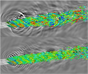
Next, we present the instantaneous vortical structures within the jet plume, as identified by the $Q$-criterion, with the background illustrated by the velocity divergence, as depicted in figure 14. Compared with the baseline case, the oscillation of vortex structures in the $y$-direction is significantly reduced in the cases of $(4{\rm \pi}, 0.5, 0.0015)$ and $(4{\rm \pi}, 0.5, 0.0094)$. For each controlled case, the amplified forcing perturbs the vortex structures inherent to the flow field, leading to a proliferation of smaller, more fragmented vortices. However, the ability of the forcing to sustain amplification downstream determines the extent of change in the sound-production structures in the original flow field, thereby facilitating the observation of increasingly fragmented vortices at extended streamwise locations, particularly in the case of $(4{\rm \pi}, 0.5, 0.0015)$. Recognizing that the introduction of forcing will inevitably alter the sound-producing energetic structures and potentially generate new sound-producing structures, we combined standard and acoustic resolvent analyses to inform our control strategies previously.

Figure 14.

The instantaneous vortex structures in the jet plume with the $Q$-criterion $(Q=1)$ coloured by longitudinal velocity $v$ and the background is shown by the divergence of velocity for (a) baseline and (b–d) controlled cases.

The far-field acoustic response of near-field structures for different cases is demonstrated using the PSD of pressure fluctuations, as shown in figure 15. In the upstream direction (monitoring point M1), the case of $(4{\rm \pi}, 0.5, 0.0094)$ shows a reduction of the screech peak by more than 10 dB compared with the baseline case. Additionally, the screech harmonics $(2St_s)$ and higher harmonics $(3St_s, 4St_s,\ldots )$ are also significantly suppressed. In our planar screeching jet, there is no complex staging behaviour, and the generation of the screech is related to the primary shock wave number peak (Edgington-Mitchell et al. Reference Edgington-Mitchell, Li, Liu, He, Wong, Mackenzie and Nogueira2022; Nogueira et al. Reference Nogueira, Jaunet, Mancinelli, Jordan and Edgington-Mitchell2022a). Therefore, the reduction in mean shock-cell spacing also results in a higher screech frequency. Furthermore, a high-frequency peak at $St=1.0$ is observed, which corresponds to the harmonic noise of the forcing frequency $(St_f=0.5)$. The imposition of forcing inevitably introduces some actuation noise. For the case of $(4{\rm \pi}, 0.5, 0.0094)$, both the screech frequency and the harmonic peak values are somewhat reduced, but to a much lesser extent compared with the case of $(4{\rm \pi}, 0.5, 0.0015)$. Moreover, more high-frequency peaks $(St\geq 1.0)$ are observed. In the case of $(2{\rm \pi}, 1.13, 0.0015)$, not only is the reduction in screech frequency and harmonic peak values less significant but also a large number of high-frequency peaks $(St>1.0)$ are detected. This suggests the presence of strong nonlinear interactions between the forcing and the flow field structures for the case of $(2{\rm \pi}, 1.13, 0.0015)$. In the downstream direction (monitoring point M3), the noise reduction effectiveness of the cases of $(4{\rm \pi}, 0.5, 0.0015)$ and $(4{\rm \pi}, 0.5, 0.0094)$ is generally better compared with the case of $(2{\rm \pi}, 1.13, 0.0015)$. This is attributed to the more fragmented vortex structures observed in their flow fields.

Figure 15.

The PSD of pressure fluctuations at the monitoring point (a,c,e) M1 $(x/h,y/h,z/h)=(-0.39,0.85,0)$ and (b,d,f) M3 $(x/h,y/h,z/h)=(30.13,10,0)$.

4.3. Impact on the self-sustained resonance loops

In the previous subsection, we have found that active control can effectively suppress screech tones and provided an explanation based on the near-field flow characteristics. Here, we delve deeper into the mechanisms of screech noise suppression. The generation of screech has been extensively studied, with various works contributing to the understanding of this phenomenon (Merle Reference Merle1956; Raman Reference Raman1997; Gojon, Bogey & Mihaescu Reference Gojon, Bogey and Mihaescu2018; Li et al. Reference Li, Zhang, Hao and He2020b; Edgington-Mitchell et al. Reference Edgington-Mitchell, Li, Liu, He, Wong, Mackenzie and Nogueira2022). The concept of self-sustained resonance loops is widely used to account for the screeching in supersonic jets (Powell Reference Powell1953; Tam Reference Tam1995). These resonance loops typically consist of four distinct processes (Edgington-Mitchell Reference Edgington-Mitchell2019): a downstream-travelling wave; a downstream-reflection mechanism; an upstream-travelling wave; a receptivity mechanism near the nozzle lip. The downstream-travelling wave is primarily characterized by K-H instability wave packets, which originate from shear layer instabilities and are sustained by continuously extracting energy from the mean flow. The upstream-travelling wave mainly comprises guided jet waves that propagate within the shear layer, formed through the interaction of shock waves and vortices in the downstream reflection process. This upstream wave excites new instability waves near the nozzle lip, thereby closing the resonance loop. In addition to the K-H instability waves and guided jet waves within the shear layer, trapped waves confined in the jet core by the shear layer also play a significant role in the resonance loops. The resonance loop can be visually observed in the schematic diagram in figure 16.

Figure 16.

Schematic of an underexpanded supersonic jet.

Since the generation of screech is closely related to the wave propagation characteristics in the jet plume, the frequency–wavenumber spectra of pressure fluctuations, obtained through spatiotemporal Fourier transform along the lines $(y/h, z/h)=(0.5, 0)$ and $(0, 0)$, are depicted in figures 17 and 18, respectively. In figure 17, positive and negative wavenumbers represent waves propagating downstream and upstream, respectively. The red dashed line indicates the approximate convective velocity $(0.6U_j)$ of the K-H instability waves (Liang et al. Reference Liang, Wan, Ye, Zhang, Sun and Lu2023). For the baseline case, distinct energy peaks appear at $St=0.11$, $0.22$ and $0.33$, corresponding to the screech frequency and its harmonics. The downstream-propagating K-H instability wave packet, marked by the red line, also exhibits significant energy. These waves, both upstream and downstream propagating, substantially contribute to the generation of screech tones. For the case of $(k_zh, St_f, C_{\mu })=(4{\rm \pi},0.5,0.0015)$, energy peaks manifest at $St=0.5$ and $1.0$, corresponding to the forcing frequency and its harmonic. The energy of the waves corresponding to the screech frequency and its harmonics is significantly reduced, suggesting that the nonlinear interactions in the flow field are weakened and the screech resonance loops are mitigated. In contrast, for the cases of $(4{\rm \pi}, 0.5, 0.0094)$ and $(2{\rm \pi}, 1.13, 0.0015)$, the energy of waves associated with the screech frequency and its harmonics remains at a relatively high level. In figure 18, similar findings to those in figure 17 can be found. Especially for the screech harmonics, the energy amplitude is significantly suppressed compared with the uncontrolled case and the $(k_z h, St_f, C_{\mu })=(4{\rm \pi},0.5,0.0015)$ case, which corresponds to the substantial suppression of screech harmonic noise in figure 15(a). This phenomenon is mainly related to the suppression of the screech harmonic mode (varicose mode), which will be further discussed in the next subsection. The upstream and downstream propagating waves in the jet core region are most effectively suppressed in the case of $(k_z h, St_f, C_{\mu })=(4{\rm \pi},0.5,0.0015)$. We can conclude that the sustained amplification of forcing in the streamwise direction can weaken the upstream and downstream wave processes within the resonance loops, thereby suppressing the generation of screech noise.

Figure 17.

Frequency–wavenumber spectra of the pressure fluctuation for four cases along the straight line of $(y/h, z/h)=(0.5, 0)$. The greyscale range is logarithmic and the red dashed line indicates the group velocity of the K-H instability waves.

Figure 18.

Frequency–wavenumber spectra of the pressure fluctuation for four cases along the straight line of $(y/h, z/h)=(0, 0)$. The greyscale range is logarithmic.

4.4. Impact on the coherent structures

The convection and oscillation of coherent turbulent structures in the jet shear layer and their interaction with shock waves in the jet plume are often accompanied by intense noise. These noise sources are non-compact, resulting in significant directivity of the noise (Papamoschou Reference Papamoschou2018; Prasad & Unnikrishnan Reference Prasad and Unnikrishnan2024b). Identifying the dynamic behaviour of near-field coherent structures is beneficial for understanding the far-field noise radiation characteristics. Therefore, the influence of control on near-field coherent structures needs to be investigated using the 3-D SPOD method (Towne et al. Reference Towne, Schmidt and Colonius2018), which is performed in a subdomain of $0\leq x/h\leq 20$, $-2.5\leq y/h\leq 2.5$ and $-2.5\leq z/h\leq 2.5$.

The comparison of the eigenvalue spectra between the baseline and controlled cases for the leading two SPOD modes is shown in figures 19(a) and 19(b). In the leading SPOD mode, for the baseline jet, peaks appear at the screech frequency $(St = 0.113)$ and its harmonics $(St = 0.226, 0.339, \ldots )$. Considering the controlled case with $(k_zh, St_f, C_{\mu })=(4{\rm \pi},0.5,0.0015)$, peaks are induced at the forcing frequency, $St_f = 0.5$, and its harmonic, $St = 1.0$, while screech-related peaks are well suppressed. The amplification of forcing in the streamwise direction extracts energy from the mean flow and engages in nonlinear interactions within the flow field, altering the growth of screech-related wave packets in the original flow field. This causes the energy of the screech-related coherent structures to shift to the higher forcing frequency and its harmonics. For the case of $(4{\rm \pi},0.5,0.0094)$, the screech peak magnitude is reduced compared with the baseline case, and peaks at the forcing frequency and its harmonic are also observed. However, the peak magnitudes at the forcing frequency and its harmonics are slightly smaller than those in the case of $(4{\rm \pi},0.5,0.0015)$. This is attributed to the result that lower amplitude forcing results in more sustained amplification in the streamwise direction. In the second SPOD mode, the effect of control is relatively minor, and forcing peaks do not appear.

Figure 19.

The comparison of the eigenvalue spectra between the baseline and controlled cases for the first two most energetic modes.

It is worth emphasizing that for the noise reduction mechanisms, the nonlinear interactions induced by forcing should be critically important. This viewpoint is quantitatively supported by the global stability analysis results for the baseline and controlled cases, as shown in table 1. In the resolvent framework, the application of the actuation signal primarily affects the mean flow and the nonlinear characteristics of the flow system. However, the results of table 1 indicate that the growth rate of the screech mode did not significantly decrease, and even increased for the case with the best noise reduction effect. This suggests that changes in the linear response of mean flow cannot explain the noise control mechanism. It also implies that the nonlinear interactions induced by the forcing not only alter the mean flow but also significantly impact the nonlinear characteristics of the flow system. Nonlinear interactions in combination of the modified mean flow should play a dominant role in noise control.

Table 1.

Growth rates obtained through global stability analysis for baseline and controlled cases.

To investigate the impact of control on coherent structures, the spatial support of the leading SPOD modes at three representative frequencies (screech frequency, screech harmonic and forcing frequency) is shown in figure 20. At the screech frequency, antisymmetric modes are observed in all cases, which are induced by shear layer flapping. However, compared with the baseline case, the spanwise coherent structures in the cases with better noise reduction (the case of $(k_z h, St_f, C_{\mu })=(4{\rm \pi},0.5,0.0015)$) become more distorted and fragmented, which can also be observed in the two-dimensional spanwise-decomposed Fourier modes. At the screech harmonic frequency, a symmetric mode is found in the baseline case, consistent with the observations of Tam & Norum (Reference Tam and Norum1992). The generation of the symmetric mode is attributed to the varicose motions of the jet shear layer. In all controlled cases, particularly for the case of $(k_z h, St_f, C_{\mu })=(4{\rm \pi},0.5,0.0015)$, the varicose mode with large-scale spanwise structures ($k_zh=0$) is significantly suppressed. Instead, the relatively disordered turbulent structures (high spanwise wavenumber structures) are predominant, leading to significant suppression of noise at screech harmonic in figure 15(a). At the forcing frequency, the control cases transform the disordered turbulent structures in the original flow field into organized structures with the forcing frequency and wavenumber. These structures are highly energetic and gradually become fragmented as they develop downstream. The organized coherent structures in the case of $(2{\rm \pi},1.13,0.0015)$ exhibit a comparatively faster breakdown and dissipation, impeding their downstream development and resulting in less effective control of jet noise.

Figure 20.

Isolevels of the leading SPOD modes of streamwise velocity, and its spanwise decomposed Fourier modes for four different cases at the screech frequency, screech harmonics and forcing frequency. The four different cases are (a) uncontrolled, (b) $(k_z h, St_f, C_{\mu })=(4{\rm \pi},0.5,0.0015)$, (c) $(4{\rm \pi},0.5,0.0094)$ and (d) $(2{\rm \pi},1.13,0.0015)$. Contour levels are uniformly set to $\pm 0.01$.

It is worth emphasizing that the control framework based on resolvent analysis is grounded in linear assumptions, and the actual control process cannot apply global forcing in the flow field. This discrepancy may lead to differences between the amplification characteristics from the applied forcing and the resolvent response modes. While the resolvent analysis may occasionally deviate from expectations under certain parameter conditions, it still identifies effective control parameter ranges at a significantly lower cost than numerical simulations and experiments. To perform detailed evaluations within these parameter spaces using simulations or experiments would be more efficient and faster.