
1. Introduction
The ground beneath our feet forms a porous matrix of permeable soil and rock, capable of storing water, called an ‘aquifer’ (Bierman & Montgomery Reference Bierman and Montgomery2014). Near the surface, this matrix is only partially saturated with water. With depth, however, the proportion of water increases until the pores are fully saturated, and the groundwater pressure exceeds the atmospheric pressure (Dunne Reference Dunne1990). The water table, i.e. the interface that separates the unsaturated zone from the saturated zone, is a dynamic boundary, whose shape changes over time (Shercliff Reference Shercliff1975; Alley et al. Reference Alley, Healy, LaBaugh and Reilly2002). During rainfall, water infiltrates into the ground, travels down through the unsaturated zone, and reaches the water table (figure 1). This input of water induces a pressure gradient that pushes groundwater through the aquifer, and then up into the neighbouring stream (Harrold Reference Harrold1934; Petroff et al. Reference Petroff, Devauchelle, Kudrolli and Rothman2012). Viscous friction, however, delays this transfer. Part of the rainwater thus accumulates temporarily in the aquifer, and makes the water table bulge and rise above the river level (Guérin et al. Reference Guérin, Devauchelle, Robert, Kitou, Dessert, Quiquerez, Allemand and Lajeunesse2019). Once the rain has stopped, the aquifer slowly releases this excess water into the stream. As a result, the latter continues to flow until the water table relaxes to its equilibrium shape, a horizontal surface levelled with the river.
Flow of groundwater into a river (cross-sectional view). (a) Shallow-aquifer configuration: sometimes referred to as the ‘fully penetrating stream’, the bottom of the aquifer is horizontal and joins the stream. (b) Deep-aquifer configuration: the bottom of the aquifer lies deep beneath the river bed.

A river is thus the visible manifestation of a much larger flow, most of which occurs underground (Devauchelle et al. Reference Devauchelle, Petroff, Lobkovsky and Rothman2011, Reference Devauchelle, Petroff, Seybold and Rothman2012). In particular, it is the volume of groundwater that the aquifer stores above the river which sustains the river between two rainfall events. This ‘active’ volume thus determines the hydrologic regime of the river. If it is small or, equivalently, if the return time between rainfalls is long, the water table relaxes before the next rainfall event, and the river dries up. The latter is then said to be ephemeral: it flows only over short periods of time after a rainfall event (Costigan et al. Reference Costigan, Kennard, Leigh, Sauquet, Datry and Boulton2017). Conversely, if the active volume is large enough, or if the time between rainfalls is short, the water table never returns to its equilibrium shape, and the river flows continuously (Bierman & Montgomery Reference Bierman and Montgomery2014). Therefore, in order to estimate how a changing precipitation pattern will affect the discharge of rivers, we need to identify the factors that control the active volume (Taylor et al. Reference Taylor2013; Pokhrel et al. Reference Pokhrel2021).
Obviously, the volume of groundwater stored in an aquifer increases with the duration of a rainfall event. If the event lasts long enough, the active volume eventually reaches a maximum, at which point the discharge at the aquifer outlet balances the rainfall input. This maximum storage capacity is rarely achieved in nature, where rainfall is often short. However, Horton (Reference Horton1936) proposed to use this maximum to characterise the capacity of an aquifer to store water. Following him, we now define the active volume  $V_a$ as the maximum volume of groundwater that the aquifer can store above its outlet, when submitted to a given rainfall rate. This definition makes the active volume independent of the duration of a rainfall event. It does, however, depend on the intensity of rainfalls, and on the porosity and hydraulic conductivity of the aquifer (Guérin et al. Reference Guérin, Devauchelle, Robert, Kitou, Dessert, Quiquerez, Allemand and Lajeunesse2019). It also depends on the geometry of the aquifer and its position relative to the river that drains it.
The simplest configuration is that wherein the bottom of the aquifer is horizontal and joins the stream (figure 1a). In this configuration, sometimes referred to as the ‘fully penetrating stream’, groundwater flows almost horizontally (Guérin et al. Reference Guérin, Devauchelle, Robert, Kitou, Dessert, Quiquerez, Allemand and Lajeunesse2019). The active volume thus coincides with the total volume of water in the aquifer, and the flow is amenable to the shallow-water approximation (Troch et al. Reference Troch2013). Combined with Darcy's law, the latter provides a simplified description of the flow, in the form of the Dupuit–Boussinesq equation (Dupuit Reference Dupuit1863; Boussinesq Reference Boussinesq1903). This theory, which assumes that the pressure is hydrostatic, provides an accurate description of the response of the water table to rainfalls. It accounts for the active volume of water stored in the aquifer during rainfall, and for its release in the drainage network, once the rainfall has stopped (Horton Reference Horton1936; Brutsaert & Nieber Reference Brutsaert and Nieber1977; Troch et al. Reference Troch2013; Guérin, Devauchelle & Lajeunesse Reference Guérin, Devauchelle and Lajeunesse2014; Guérin et al. Reference Guérin, Devauchelle, Robert, Kitou, Dessert, Quiquerez, Allemand and Lajeunesse2019).
In the field, however, fully penetrating streams are not the norm, and the base of the aquifer often lies deep below the stream that drains it (figure 1b). Groundwater must therefore rise to reach the stream, and the vertical component of the flow violates the Dupuit–Boussinesq approximation (Lehr Reference Lehr1963; Haria & Shand Reference Haria and Shand2004). In this configuration, which we call ‘deep aquifer’, the hydraulic head that drives the flow obeys Laplace's equation, the solution of which depends on the boundary conditions (Polubarinova-Kochina Reference Polubarinova-Kochina1962). The aquifer is usually bounded by a quasi-horizontal impervious layer at its base. Below the river, groundwater converges from both sides, forming a convergent groundwater divide (figure 1b). Since groundwater does not cross this boundary, it is modelled as a vertical impervious wall. Farther from the river, the groundwater flow changes direction, and eventually moves towards a different stream (figure 1b). The surface where this bifurcation occurs forms a divergent drainage divide, which, like the convergent one, can be represented as an impervious vertical wall (Toth Reference Toth1963). The last boundary is the water table, which freely adjusts its shape to accommodate the rainfall input. One thus needs to solve Laplace's equation inside a domain that is a priori unknown. This free-boundary problem requires two boundary conditions at the water table. In addition to equating the groundwater pressure with the atmospheric one, one must also account for the flux of rainwater that reaches the water table. In short, determining the flow inside an aquifer recharged by rainfall is a Stefan problem: the values of both the hydraulic head and its derivative are specified at the water table, the shape of which must be solved for.
Jules et al. (Reference Jules, Lajeunesse, Devauchelle, Guérin, Jaupart and Lagrée2021) investigated this problem in a deep two-dimensional laboratory aquifer recharged by artificial rain. After a short transient, the water table adjusts so that the discharge at the aquifer outlet equilibrates the rainfall input. For small rainfall rates, the water table barely departs from the horizontal. Based on this observation, Jules et al. (Reference Jules, Lajeunesse, Devauchelle, Guérin, Jaupart and Lagrée2021) linearised the boundary condition at the free surface and, thus, bypassed the difficulty of the Stefan problem. The resulting theory provides an analytical expression for the shape of the streamlines in steady state (Jules et al. Reference Jules, Lajeunesse, Devauchelle, Guérin, Jaupart and Lagrée2021). Yet, the linearisation of the boundary condition at the water table comes at a cost: it reduces the aquifer outlet to a point, where the hydraulic head diverges. This has an unexpected consequence: the linear theory predicts that the active volume of water stored in the aquifer is exactly zero (Jules et al. Reference Jules, Lajeunesse, Devauchelle, Guérin, Jaupart and Lagrée2021). In short, the theory fails to account for the active volume. To estimate it, we thus need to solve the original, nonlinear Stefan problem.
As far as we know, the shape of the water table in a deep aquifer recharged by rainfall remains an open question. Following Jules et al. (Reference Jules, Lajeunesse, Devauchelle, Guérin, Jaupart and Lagrée2021), we address this problem in a laboratory aquifer recharged by artificial rain. Jules et al. (Reference Jules, Lajeunesse, Devauchelle, Guérin, Jaupart and Lagrée2021), however, restricted their investigation to small rainfall rates, for which the water table barely deviates from the horizontal. Here, in contrast, we investigate a broader range of rainfall rates, for which the water table deforms significantly. We begin with a description of the experimental set-up (§ 2). We then focus on the steady-state regime, for which the discharge at the outlet balances the rainfall input, and examine how the groundwater pressure and the active volume of water stored in the aquifer vary with the rainfall rate and the hydraulic conductivity of the porous material (§ 3). To better constrain the flow, we introduce dye in the aquifer, and track its trajectory (§ 4). This allows us to visualise the streamlines, and to constrain the shape of the water table. Based on these observations, we derive the equations of the flow (§ 5). For an infinitely deep aquifer, we find that the latter admit a closed-form solution, which represents well the pressure and the active volume in our experiment (§§ 6 and 7). Finally, we propose a numerical procedure that allows us to solve for the flow in an aquifer of finite depth, validate its predictions against our experiments, and use it to show how the active volume of water varies with the depth of the aquifer (§ 8).
2. Laboratory aquifer
Our experimental set-up is similar to that of Jules et al. (Reference Jules, Lajeunesse, Devauchelle, Guérin, Jaupart and Lagrée2021). It consists of a narrow tank formed by two vertical PMMA plates ( $90.5 \times 92\,\mathrm {cm}$), separated by a gap of width
 $W = 5\,\mathrm {cm}$ (figure 2). The tank is filled with glass beads of nearly uniform size (ranging from 0.3 to 3 mm in diameter depending on the experimental series), which form an artificial aquifer bounded by an impermeable bottom.
Experimental set-up and notation. The aquifer (length  $L =90.5\,{\rm cm}$ and depth
 $H = 63.7\,{\rm cm}$) is made of glass beads (shaded area) piled between two vertical PMMA plates (black solid lines) separated by a narrow gap (width
 $W = 5\,{\rm cm}$). When rain falls on the aquifer, the water table deforms and groundwater (in blue) flows out of the aquifer. The black dotted line indicates the level of the aquifer outlet and the equilibrium position of the water table. The volume of water above this line (dark blue) corresponds to the volume of water that the aquifer stores during rainfall (active volume).

An array of  $24$ evenly spaced needles, placed above the tank, feeds the aquifer with artificial rain. These needles, of inner diameter
 $0.8\,\mathrm {mm}$, uniformly distribute water over the aquifer's surface, with a standard deviation of about
 $3\,\%$ in discharge. The sprinkler pipe receives water from an overflowing tank. A solenoid valve (Burkert W29MA), placed between the two, allows us to start and stop the rainfall, by mean of an Arduino board operated from a computer. An electromagnetic flowmeter (Kobold MIK
 $0.05\unicode{x2013}1\,{\rm l}\,{\rm min}^{-1}$, accuracy
 $2\,\%$) measures the rainfall input,
 $Q_{in}$, from which we deduce the rainfall rate
 $R = Q_{in}/(LW)$, where
 $L = 90.5\,{\rm cm}$ is the length of our aquifer.
Two impervious vertical walls close the left and right ends of our aquifer (figure 2). The right-hand wall extends over the whole height of the tank. The left-hand wall, by contrast, extends only up to a height  $H = 63.7\,{\rm cm}$ above the aquifer's bottom. The remaining height (approximately
 $30\,\mathrm {cm}$) is covered with a permeable, vertical grid, which retains the glass beads, while allowing water to seep out of the aquifer. During rainfall, the asymmetry of these boundary conditions forces water to leave the aquifer through its left-hand side, at an elevation
 $H = 63.7\,{\rm cm}$ above the aquifer's bottom. This outlet mimics the river into which a natural aquifer would drain, and the aspect ratio of our aquifer is thus
 $a = H/L \approx 0.70$. As for the right-hand impervious wall, it plays the role of the drainage divide.
We monitor the pressure inside the aquifer, at a point located 10 cm from the drainage divide and 7.5 cm below the level of the outlet (figure 2). The horizontal and vertical coordinates of the measurement point relative to the aquifer outlet are thus  $x_p= 80.5\,{\rm cm}$ and
 $y_p = -7.5\,{\rm cm}$. This position allows us to measure pressure near, but not at, the divide, in a region where streamlines are nearly vertical (see § 4). To measure pressure, we use a SENO343 differential pressure transducer, mounted on an Arduino board connected to a computer. Because it is designed to operate in a gas, the transducer cannot be in contact with water. To bypass this issue, we drill a 5 mm hole through the lateral wall of our experimental set-up, at the measurement point, and cover it with a metallic mesh, which retains the glass beads inside the tank. A PDMS tube (diameter
 $7\,\mathrm {mm}$) connects the hole to the lower end of a small vertical cylindrical tank of height
 $7.3\,\mathrm {cm}$ and diameter
 $15.2\,\mathrm {mm}$, large enough to neglect surface tension (figure 2). The tube and the lower half of the cylindrical tank are filled with water. The upper half of the tank is filled with air, and its upper end is connected through a second tube to the pressure transducer. In this way, the transducer measures the pressure of the air, which equilibrates with that of water in the aquifer, with an offset that depends on the position of the transducer. We eliminate this offset by setting the zero of this measurement at equilibrium, after the aquifer has drained entirely. This procedure allows us to measure, every second, the pressure in the aquifer with an accuracy of
 ${\pm }0.5\,{\rm Pa}$.
The presence of air bubbles trapped between glass beads can alter the groundwater flow. To prevent this, we build our aquifer according to the following procedure. We first fill the tank with water. Using a funnel, we then gradually pour glass beads into the tank, where they settle and form a loose pile. To increase the compacity of the latter, we regularly interrupt the pouring, and gently tap the walls of the tank with a mallet. With each tap, the compacity of the pile increases, and its free surface drops. After a dozen taps, its compaction reaches a maximum. We then pour some more beads, and repeat this procedure until the upper surface of the pile of beads (i.e. the free surface of the aquifer) extends up to about 25 cm above the outlet.
We ran a total of three series of experiments, using three different types of glass beads (manufacturer: Marteau & Lemarié). In series 1 and 2, the aquifer was made of slightly heterogeneous grains, of sizes between  $300$ and
 $400\,\mathrm {\mu }{\rm m}$ (median diameter
 $d_s=350\,\mathrm {\mu } {\rm m}$) and between
 $0.8$ and
 $1.3\,{\rm mm}$ (median diameter
 $d_s=1.05\,{\rm mm}$), respectively. During series 3, we worked with quasi-homogeneous glass beads of diameter
 $3\,{\rm mm}$.
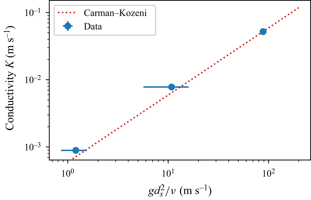
We measured the hydraulic conductivity of each type of bead, following the relaxation method of Jules et al. (Reference Jules, Lajeunesse, Devauchelle, Guérin, Jaupart and Lagrée2021). The method relies on two communicating vessels connected by a Darcy column filled with glass beads, and saturated with water. The release of a finite volume of water in one of the vessel induces a pressure gradient in the Darcy column, which drives a flow that tends to equilibrate the water levels in the two vessels. The water level in each vessel then relaxes exponentially, with a characteristic time that depends on the hydraulic conductivity  $K$ of the pack of beads. Using this method, we find the values reported in table 1, which conform to the empirical Kozeni–Carman relationship,
 $K = c g d_s^2/\nu$, where
 $d_s$ is the grain size,
 $\nu$ the kinematic viscosity of water,
 $g$ the acceleration of gravity and
 $c=5.9 \pm 0.1 \times 10^{-4}$ is a dimensionless coefficient (Carman Reference Carman1937) (Appendix A, figure 17).
Experimental parameters for each experimental series.

Finally, we also estimated the porosity of the aquifer by repeatedly weighing known volumes of dry glass beads. We found porosities ranging from  $S \approx 0.37$ to
 $S \approx 0.38$ (table 1), as expected for the random close packing of spheres (Andreotti, Forterre & Pouliquen Reference Andreotti, Forterre and Pouliquen2013).
3. Active volume and dynamic pressure
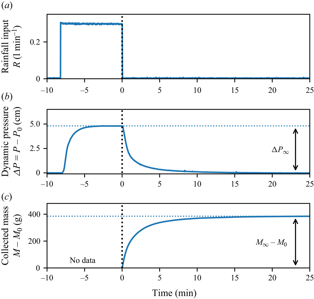
To prepare the experiment before each run, we first feed the aquifer with an arbitrary rainfall rate, until it overflows. We then stop the rain, and wait until the discharge at the outlet vanishes. In this equilibrium state, the water table is horizontal and levelled with the outlet, while pressure at the measurement point is hydrostatic, with a value denoted  $P_0$. Starting from this initial condition, we impose an artificial rain with the desired rainfall rate,
 $R$ (figure 3a). Approximately 10 s after the rain starts, the pressure begins to rise, indicating that the rainwater has reached the water table (figure 3b). As the water table bulges to accommodate this input, groundwater starts flowing and the pressure inside the aquifer gradually increases. After a transient of about two minutes, the pressure converges to a steady-state value,
 $P_\infty$, indicating that the flow is in steady state: the discharge at the aquifer outlet balances the rainfall input. Because our pressure sensor measures the pressure with an offset, the values of
 $P_\infty$ and
 $P_0$ are of little use per se (§ 2). We thus introduce the dynamic pressure
 $\Delta P = (P - P_0)$, and its steady-state value
 $\Delta P_\infty = (P_\infty - P_0)$, which represent the deviation of the pressure from hydrostatic equilibrium, and do not involve any offset (figure 3b).
Experimental run. (a) Rainfall discharge ( ${\rm l}\,{\rm min}^{-1}$), (b) dynamic pressure
 $\Delta P = P-P_0$ (in centimetres of water), and (c) mass of water collected at the aquifer outlet,
 $M-M_0$ (grams), as a function of time. Due to experimental limitations, we only measure the mass of water exiting the aquifer after the rainfall has stopped, rather than over the entire duration of an experimental run. Consequently, there are no data available for times
 $t<0$. The aquifer, made of
 $800\unicode{x2013}1300\,\mathrm {\mu }{\rm m}$ glass beads, is submitted to a rainfall input
 $Q_{in} = 0.3\,{\rm l}\,{\rm min}^{-1}$, corresponding to a dimensionless rainfall rate of
 $R/K = 0.018$. Vertical dotted line: time
 $t=0$, when rainfall stops.

Our experimental set-up does not allow us to measure directly the active volume of water stored in the aquifer. Instead, we measure the volume of water collected at the aquifer's outlet after the rainfall has stopped,  $V_{out}$, and hope that the latter provides a reliable estimate of the active volume stored in the aquifer during rainfall (figure 3c). To measure this volume, we collect the water exiting the aquifer in a bucket placed beneath the outlet. A scale located under the bucket records its weight every 0.1 s. To improve the accuracy of our measurement, we use a scale with a precision of 1 mg. However, this precision imposes a limitation: the scale cannot measure weights greater than 1200 g. As a result, we cannot measure the mass of water leaving the aquifer over the entire duration of an experimental run. Instead, we restrict our measurements to the mass of water collected after the rainfall has stopped. To do this, we apply the following procedure. The water that leaves the aquifer falls into a reservoir that recirculates it to the sprinkler. We wait until the flow is in steady state, then use a movable tray to replace the recirculating reservoir with the bucket. As long as it rains, water accumulates in the bucket at a rate equal to the rainfall input. Once the weight of water exceeds approximately
 $M_0 \sim 200$ g, we turn the rainfall off. The water table immediately starts to relax towards equilibrium. As it does, the discharge at the outlet gradually decreases towards zero, and the mass of water in the bucket reaches a plateau
 $M_\infty$ (figure 3c). The volume of water collected after the rainfall stopped is thus
 $V_{out} = (M_\infty - M_0) / \rho$, where
 $\rho$ is the density of water, and
 $M_0$ the mass of water in the bucket at the time when the rainfall stops. As the water table returns to equilibrium, so does the pressure in the aquifer, which relaxes to its hydrostatic value (figure 3b).
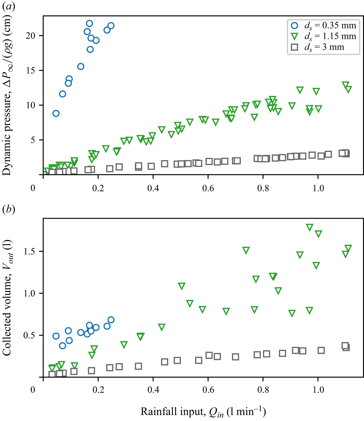
Following the above procedure, we systematically measure the dynamic pressure,  $\Delta P_\infty$, and the volume of water collected at the aquifer outlet,
 $V_{out}$, as a function of the rainfall rate, for each of the three types of glass beads presented in the previous section. As expected, we find that these two quantities increase with the rainfall rate (figure 4). For a fixed rainfall rate, the active volume and the hydraulic head increase as the hydraulic conductivity decreases. This, again, matches intuition: a decrease of the hydraulic conductivity implies a greater head loss through the aquifer. A higher pressure, and thus a higher water table, is then necessary for the groundwater discharge to equilibrate the rainfall input.
(a) Dynamic pressure (centimetres of water) and (b) volume of water collected at the aquifer outlet after the rainfall has stopped (litres) vs rainfall discharge  $Q_{in}$ (
 ${\rm l}\,{\rm min}^{-1}$). Different symbols represent different experimental series (table 1).

To understand how the active volume and the dynamic pressure depend on the rainfall rate and the hydraulic conductivity, we now turn our attention to the flow. In the next section, we describe injecting dye into the aquifer, tracking its propagation to visualise the streamlines and detecting the shape of the water table.
4. Streamlines
To visualise the water table, we impose an artificial rainfall, and monitor the pressure in the flow, as described in the previous section. After a few tens of seconds, the pressure reaches steady state. We then inject small parcels of blue dye into the aquifer, and monitor their propagation. The dye consists of a mixture of water (90 %) and food colouring (Matfer, 10 %). Its density ( $997\,{\rm kg}\,{\rm m}^{-3}$) is close enough to that of water to assume that it behaves as a passive tracer. We inject the dye into the aquifer by mean of six hypodermic needles, evenly spaced along the aquifer surface. Six flexible tubes connect each needle to a syringe, mounted on a syringe pump (SPLab06, Schenchen Baoding), which allows us to simultaneously inject small volumes of blue dye (0.5 ml) through the six needles.
The six parcels of dye travel through the aquifer until they eventually reach the outlet, where they exit the aquifer. A camera facing the set-up records an image of the position of the dye parcels every 15 s. A LED panel, placed behind the aquifer, increases the contrast of the image. Once all parcels have left the aquifer, we stop the camera and merge all the pictures (approximately 250 images) into a single one, that keeps, for each pixel, its darkest value over the course of the experiment. The resulting image reveals the trajectories of the parcels of dye, in the form of six blue stripes (figure 5).
Trajectories of six parcels of dye in the experimental aquifer, revealed by merging 250 pictures into one, keeping at each point the darkest pixel. The aquifer, made of  $800\unicode{x2013}1300\,\mathrm {\mu }{\rm m}$ glass beads, is subjected to a rainfall input
 $Q_{in} = 1.15\,{\rm l}\,{\rm min}^{-1}$, corresponding to a dimensionless rainfall rate
 $R/K=0.07$. Orange, blue and black dashed lines show the seepage face, water table and streamlines computed from the numerical procedure presented in § 8.

Jules et al. (Reference Jules, Lajeunesse, Devauchelle, Guérin, Jaupart and Lagrée2021) used a similar procedure to visualise the streamlines in an aquifer submitted to an artificial rainfall, with two important differences. First, Jules et al. (Reference Jules, Lajeunesse, Devauchelle, Guérin, Jaupart and Lagrée2021) restricted their investigation to small rainfall rates,  $R/K \lesssim 4\times 10^{-3}$, for which the water table barely deviates from the horizontal. Here, in contrast, we explore higher rainfall rates, up to
 $R/K \sim 0.1$, which deform the water table significantly. Second, Jules et al. (Reference Jules, Lajeunesse, Devauchelle, Guérin, Jaupart and Lagrée2021) injected the dye as close as possible to the water table, to minimise its journey through the unsaturated zone. Here, we inject the dye far above the water table, in an area that is not saturated with water, in the hope that the shape of its trajectory will help us locate the water table.
In the unsaturated zone, a parcel of dye travels under the sole action of gravity. We therefore expect it to follow a vertical trajectory, until it reaches the water table. This is indeed what we observe for all trajectories, except for the left-most dye stream, which is slanted slightly (figure 5). We suspect that this anomalous behaviour might result from the flow of residual air trapped inside the aquifer by the incoming rainfall. We have, however, no observation in support of this hypothesis.
As the parcels of dye enter the saturated zone, their trajectories deviate from the vertical, and follow an arcuate path towards the outlet (figure 5). This abrupt change of direction allows us to locate the water table. It coincides with a slight change of colouration of the aquifer, probably due to its saturation with water. As expected, the elevation of the water table is maximum at the drainage divide (right wall), and gradually decreases towards the outlet, where it forms a seepage face, which extends a few centimetres above the bottom of the outlet.
Once in the saturated zone, the trajectory of the dye depends on the position of the injection point. Parcels injected near the outlet stay above it throughout their trajectory: they descend continuously from the water table down to the outlet. Parcels injected far from the outlet have a different fate: they move downwards and get below the outlet, until they eventually rise again, and flow towards the seepage face, where they exit the aquifer (figure 5).
The injection of dye has allowed us to observe the flow streamlines and to visualise the shape of the water table. In the next section, we use these observations to derive the flow equations.
5. Flow equations
5.1. Physical space
Below the water table, groundwater flows according to Darcy's law,
 \begin{equation} \boldsymbol{q} ={-} K \boldsymbol{\nabla} \left( \frac{p}{\rho g} + y \right) , \end{equation}
where  $\rho$ is the density of water,
 $P$ is the pressure and
 $\boldsymbol {q}$ is Darcy's velocity. This velocity, also referred to as Darcy's flux, represents the volumetric flux of water through a unit cross-sectional area of porous medium. The horizontal and vertical coordinates,
 $x$ and
 $y$, are measured with respect to the position of the aquifer's outlet (figure 2). In steady state, combining Darcy's law and incompressibility yields Laplace's equation
 \begin{equation} \nabla^2\phi = 0 , \end{equation}
where we introduce the hydraulic head,  $\phi = p/\rho g + y$. This quantity measures the deviation of the pressure from hydrostatic equilibrium, expressed in height of water.
To solve (5.2), we first assume that the flow does not vary across the experiment. This assumption reduces our problem to a two-dimensional flow in the  $(x,y)$ plane. Because the solutions of Laplace's equation are complex analytical functions, we introduce the complex potential
 $\varPhi (z) = \phi + {\rm i} \psi$, where
 $\psi$ is the stream function associated with this Darcy flow,
 $z =x+{\rm i}y$ is the complex coordinate and
 $i^2=-1$ (Polubarinova-Kochina Reference Polubarinova-Kochina1962). As long as
 $\varPhi$ is an analytical function of
 $z$, its real (and imaginary) part obeys Laplace's equation (5.2).
To determine the expression of the complex potential  $\varPhi$, we need to complement (5.2) with boundary conditions. We first note that the three walls that bound the aquifer are impervious, so that the normal velocity of groundwater vanishes along them. These walls thus form a streamline, along which the value of the stream function
 $\psi$ is constant. By arbitrarily setting the latter to zero, this boundary condition translates into
 \begin{equation} \psi=0 \end{equation}
along the right, bottom and left walls (figure 6a).
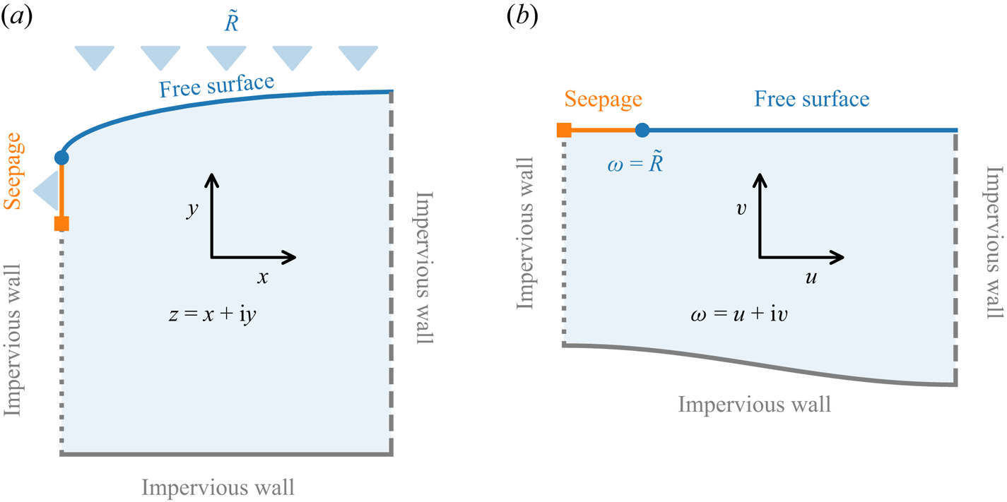
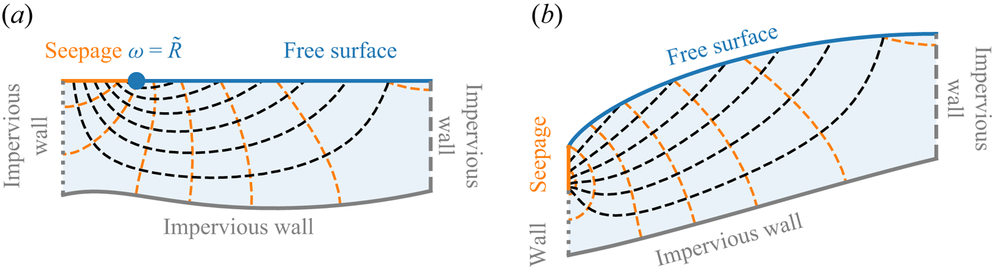
Conformal mapping from the physical plane (a) to the mathematical one (b). Coordinates in the physical (respectively, mathematical) plane are represented by  $z=x+{\rm i}y$ (respectively,
 $\omega = u +{\rm i}v$). Laplace's equation is solved within the shaded domain. Coloured lines represent the different boundaries of the problem, as indicated in the legend.

Along the permeable grid, at the outlet, groundwater forms a seepage face, a few centimetres high, through which water flows out of the aquifer (figure 5). Along this seepage face, the pressure of water matches the atmospheric one. Arbitrarily setting the latter to zero, this condition reads
 \begin{equation} \phi=y. \end{equation}
We now turn our attention to the water table. On this free surface of elevation  $y = h(x)$, the pressure is atmospheric, so that
 \begin{equation} \phi=y. \end{equation}
The water table, however, is a free boundary which deforms to accommodate the input of water during rainfall. It thus requires an additional condition, provided by the mass balance across the water table (Jules et al. Reference Jules, Lajeunesse, Devauchelle, Guérin, Jaupart and Lagrée2021). For an homogenous rainfall, and in steady state, this condition reads
 \begin{equation} \psi = \frac{RL}{K} \left( 1 - \frac{x}{L}\right) . \end{equation}
This equation simply states that the quantity of water entering the aquifer increases linearly with the distance to the drainage divide. Combined with boundary conditions (5.3) and (5.4), it imposes that the stream function increases by an amount  $[\psi ] = RL/K$ over the seepage face, so that the discharge of water leaving the aquifer matches the total rainfall input,
 $Q = KW [\psi ] = WRL$.
The set of equations (5.2), (5.3), (5.4), (5.5) and (5.6) describes the flow in a two-dimensional aquifer recharged by rainfall (figure 6a). Introducing the dimensionless complex coordinate  $\tilde {z} = z/L$ and the dimensionless complex potential
 $\tilde {\varPhi } = \varPhi /L$, our set of equations becomes
 \begin{equation} \nabla^2\tilde{\varPhi} = 0, \end{equation}
with boundary conditions
 $$\begin{gather} \tilde{\psi} = 0 \quad \text{on the bottom } (\tilde{y} ={-}a), \end{gather}$$
 $$\begin{gather}\tilde{\psi}= 0 \quad \text{on the divide } (\tilde{x} = 1), \end{gather}$$
 $$\begin{gather}\tilde{\psi} = 0 \quad \text{on the wall below the outlet } (\tilde{x} = 0, \tilde{y} < 0), \end{gather}$$
 $$\begin{gather}\tilde{\phi} = \tilde{y}\quad \text{on the seepage face } (\tilde{x} = 0, \tilde{y} > 0), \end{gather}$$
 $$\begin{gather}\tilde{\phi} = \tilde{y} \quad \text{and } \psi = \tilde{R} (1-\tilde{x}) \quad \text{on the water table } (0<\tilde{x} <1, \tilde{y} = \tilde{h}(\tilde{x})) . \end{gather}$$
In this dimensionless form, the flow depends on only two parameters: the aspect ratio of the aquifer,  $a = H/L$, and the dimensionless rainfall rate,
 $\tilde {R} = R/K$. As far as we know, this free boundary problem does not admit any closed-form solution. In the next section, we use conformal mapping to transform it into a simpler problem.
5.2. Mapping
Inspired by Zhukovsky (Reference Zhukovsky1932) and Jules (Reference Jules2020), we introduce the dimensionless complex variable,  $\omega = u+{\rm i}v$, such that
 \begin{equation} \omega = \tilde{z}- {\rm i}\tilde{\varPhi} , \end{equation}
or, equivalently,
 $$\begin{gather} u = \tilde{x}+\tilde{\psi}, \end{gather}$$
 $$\begin{gather}v =\tilde{y}-\tilde{\phi}. \end{gather}$$
Equation (5.13) maps our physical aquifer (figure 6a) into a mathematical one, that takes the shape displayed in figure 6(b). We must now look for an analytical function  $\tilde {z}(\omega )$ that satisfies the boundary conditions along the boundaries of the mathematical aquifer:
 $$\begin{gather} \tilde{x} = u \quad \text{and } \tilde{y} ={-}a \quad \text{on the bottom}, \end{gather}$$
 $$\begin{gather}\tilde{x} = 1 \quad \text{on the divide } (u= 1, v < 0), \end{gather}$$
 $$\begin{gather}\tilde{x} = 0 \quad \text{on the wall below the outlet } (u= 0, v < 0), \end{gather}$$
 $$\begin{gather}\tilde{x} = 0 \quad \text{on the seepage face } (0< u< \tilde{R}, v= 0), \end{gather}$$
 $$\begin{gather}\tilde{x} = \frac{u-\tilde{R}}{1-\tilde{R}} \quad \text{on the water table } (\tilde{R}< u< 1, v= 0). \end{gather}$$
If we find such an analytical function, we will just need to invert it, to recover the complex potential that describes the flow in the physical space,  $\tilde {\varPhi } = {\rm i}(\omega -\tilde {z})$.
The advantage of this transformation is that it maps the seepage face and the water table on the horizontal axis  $v=0$, where the seepage face extends from
 $u = 0$ to
 $u=\tilde {R}$, and the water table from
 $u=\tilde {R}$ to
 $u=1$. The free surface is now fixed. Similarly, the left and right walls of the aquifer are mapped on two vertical lines located in
 $u=0$ and
 $u=1$, respectively. Yet, the problem retains a free boundary: the location of the aquifer bottom in the mathematical plane is unknown, which prevents us from deriving a closed-form solution. In §§ 6 and 7, we bypass this issue by successively considering two asymptotic configurations. We begin with a discussion of the flow behaviour near the aquifer outlet. There, the flow is insensitive to the boundary conditions at the bottom (5.16) and on the divide (5.17), and admits a closed-form solution (§ 6). In § 7, we reintroduce the drainage divide into the problem, and address the case of an infinitely deep aquifer. In this asymptotic configuration, (5.16) is absent from the problem, which admits a closed-form solution (§ 7).
6. Flow near the aquifer's outlet
Close enough to the outlet, the flow is insensitive to the boundary conditions at the bottom (5.16) and on the divide (5.17), and the boundary conditions reduce to
 $$\begin{gather} \tilde{x} = 0 \quad \text{on the wall below the outlet } (u= 0, v < 0), \end{gather}$$
 $$\begin{gather}\tilde{x} = 0 \quad \text{on the seepage face } (0< u< \tilde{R}, v= 0), \end{gather}$$
 $$\begin{gather}\tilde{x} = \frac{u-\tilde{R}}{1-\tilde{R}} \quad \text{on the water table } (\tilde{R}< u< 1, v= 0). \end{gather}$$
Finding an analytical function  $\tilde {z}(\omega )$ that satisfies these conditions is challenging, due to the dependency of the last boundary condition on the variable
 $u = {\rm Re}(\omega )$. To bypass this issue, we look for
 $\tilde {z}'(\omega )$, the derivative of
 $\tilde {z}(\omega )$, instead of
 $\tilde {z}(\omega )$ itself. To do this, we introduce the intermediate function
 $\chi (\omega ) = (1-\tilde {R})\,\tilde {z}'$. Both
 $\tilde {z}(\omega )$ and its derivative
 $\tilde {z}'(\omega )$ are analytical, so that our intermediate function
 $\chi (\omega )$ is also analytical. The latter satisfies the following boundary conditions:
 $$\begin{gather} {\rm Im}(\chi)= 0 \quad \text{on the wall below the outlet,} \end{gather}$$
 $$\begin{gather}{\rm Re}(\chi)= 0 \quad \text{on the seepage face,} \end{gather}$$
 $$\begin{gather}{\rm Re}(\chi) = 1 \quad \text{on the water table.} \end{gather}$$
This system of equation admits the following solution
 \begin{equation} \chi = \frac{{\rm i}}{\rm \pi} \log\left( \frac{\tilde{R} + \omega}{\tilde{R} - \omega}\right) . \end{equation}
Integrating the above equation yields an explicit expression for  $\tilde {z}$,
 \begin{equation} \tilde{z} = \frac{{\rm i}}{{\rm \pi} (1-\tilde{R} )} [ (\tilde{R} -\omega) \log(\tilde{R} -\omega) + (\tilde{R} +\omega) \log(\tilde{R} +\omega) - 2\tilde{R} \log \tilde{R}], \end{equation}
where we have fixed the origin by setting  $\tilde {z} = 0$.
For any position  $\omega$ in the mathematical plane, (6.8) yields the corresponding position
 $\tilde {z}$ in the physical space, from which we deduce the value of the complex potential
 $\tilde {\varPhi }$ using (5.13). This allows us to draw the streamlines and the water table near the aquifer outlet (figure 7). Their shape is qualitatively consistent with the experimental observations of figure 5.
Flow near the aquifer outlet. The rainfall rate is  $R/K = 0.2$. (a) Mathematical plane,
 $\omega = u+{\rm i}v$. (b) Physical plane,
 $\tilde {z} = x/L +{\rm i}y/L$. Orange dashed lines: isoheads. Black dashed lines: streamlines.

Setting  $\omega = \tilde {R}$ in (6.8) yields the height of the seepage face,
 \begin{equation} \widetilde{h_s} = \frac{2 \log 2}{\rm \pi} \frac{\tilde{R}}{1-\tilde{R} } . \end{equation}
In the limit of vanishing rainfall rate, this height is proportional to discharge, and therefore to the rainfall rate:  $\tilde {h}_s = 2 \log (2) \tilde {R} / {\rm \pi}$. The free surface is then a flow line (
 $\psi = \tilde {R}$), and all the groundwater injected at infinity flows through the seepage face. In this limit, our problem becomes a special case of the ‘drainage ditch’ discussed by Polubarinova-Kochina (Reference Polubarinova-Kochina1962, p. 166).
To gain a more comprehensive understanding of how the seepage face constrains the flow in the aquifer, we expand (6.8) under the condition of a small rainfall rate, and at a distance from the outlet large enough to ensure that  $\tilde {R}/\omega$ is small. Assuming that
 $0 < \tilde {R}/\omega \ll \tilde {R} \ll 1$, we find that (Appendix B)
 \begin{equation} \tilde{\varPhi} \sim \frac{2}{\rm \pi} \tilde{R} \log\tilde{z} , \end{equation}
or, equivalently,
 \begin{equation} \tilde{\varPhi} \sim \widetilde{h_s} \log\tilde{z} , \end{equation}
since the elevation of the seepage face is proportional to the discharge  $\tilde {R}$ for vanishing rainfall rates. Equations (6.10) and (6.11) tell us that, far from the outlet, the flow perceives the seepage face as a sink point, which generates a logarithmic singularity. As the flow approaches the aquifer outlet, it becomes sensitive to the finite size of the seepage face, and one must use the full solution (6.8).
Equations (6.8), (6.9), (6.10) and (6.11) describe the behaviour of the flow close to the aquifer outlet. They cannot, however, represent the flow in regions where the influence of the drainage divide becomes significant. In the next section, we therefore reintroduce the drainage divide into the problem, and address the case of an infinitely deep aquifer.
7. Infinitely deep aquifer
7.1. Potential, streamlines, and water table
To describe the flow in an aquifer of infinite depth, we only need to add the boundary condition at the divide (5.17) to the set of conditions that govern the problem discussed in § 6. Jules (Reference Jules2020) showed that, with this additional condition, the flow admits the following closed-form solution (Appendix C):
 \begin{align} \tilde{z} (\omega ) &=
\omega + \frac{1}{{\rm \pi}^2(1-\tilde{R})} \nonumber\\ &\quad
\times[ \text{Li}_2( {\rm e}^{-{\rm i}{\rm \pi}
(\omega +\tilde{R})} ) - \text{Li}_2( {\rm
e}^{-{\rm i}{\rm \pi} (\omega -\tilde{R})} )+
\text{Li}_2( {\rm e}^{{\rm i}{\rm \pi}\tilde{R}}) -
\text{Li}_2( {\rm e}^{-{\rm i}{\rm \pi} \tilde{R}})], \end{align}
where  $\text {Li}_2$ denotes Spence's function, sometimes referred to as ‘dilogarithm’ (Appendix C). For any position
 $\omega$ in the mathematical plane, (7.1) yields the corresponding position
 $\tilde {z}$ in the physical space, from which we deduce the value of the complex potential
 $\tilde {\varPhi }$ using (5.13).
Figure 8 shows the streamlines and the water table drawn after (7.1). Near the outlet, the water table aligns closely with the predictions of the near-outlet solution (6.8) (figure 8b). However, as the distance to the outlet increases, the two models depart from each other, and the near-outlet solution gradually overestimates the elevation of the water table.
Flow in an aquifer of infinite depth submitted to a rainfall rate  $R/K = 0.3$. (a) Mathematical plane,
 $\omega = u+{\rm i}v$. (b) Physical plane,
 $\tilde {z} = x/L +{\rm i}y/L$. Orange dashed lines: isoheads. Black dashed lines: streamlines. Dotted red line: water table predicted from the near-outlet solution (6.8).

In an aquifer of infinite depth, streamlines that originate close to the drainage divide extend to infinity, preventing any quantitative comparison with the experimental streamlines of figure 5. Yet (7.1) retains much of the experimental behaviour: (i) the depth reached by a streamline increases as its origin approaches the drainage divide (where it diverges); (ii) the water table is highest at the drainage divide, and gradually drops towards the outlet, where it forms a seepage face (figure 8).
7.2. Dynamic pressure
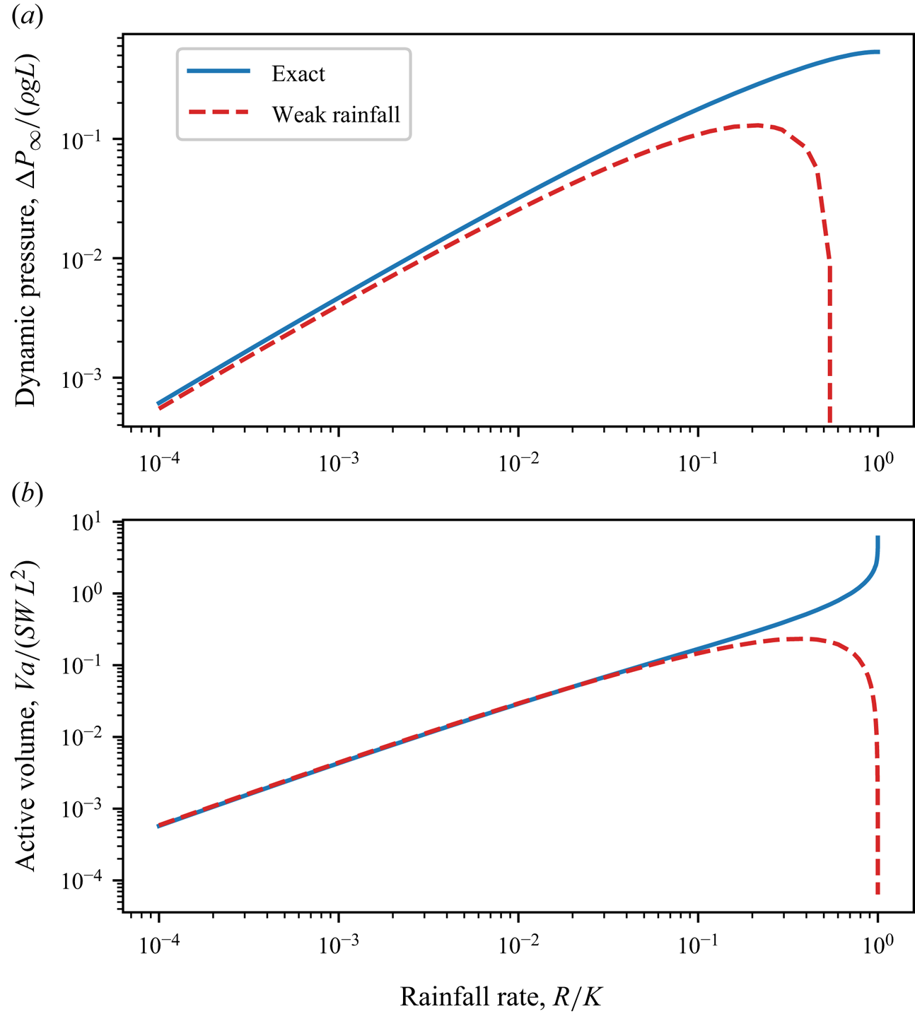
Based on (7.1), we compute the dynamic pressure,  $\Delta P_\infty /( \rho g L)$, at the position
 $(x_p, y_p)$ of the pressure probe in our experiment, and plot it as a function of the dimensionless rainfall rate,
 $R/K$. As expected, we find that the dynamic pressure in the aquifer increases with the rainfall rate (figure 9a).
(a) Dynamic pressure and (b) active volume of water stored in an aquifer of infinite depth, as a function of the rainfall rate. The dynamic pressure is evaluated in  $x_p/L=0.805$ and
 $y_p/L=-0.075$, the coordinates of the pressure probe in our experimental aquifer. Solid blue line: exact solution. Dashed red line: weak-rainfall approximation.

To compare our measurements with the infinitely deep aquifer theory, we rescale our pressure data with respect to the characteristic pressure  $\rho g L$, and plot the result as a function of the dimensionless rainfall rate
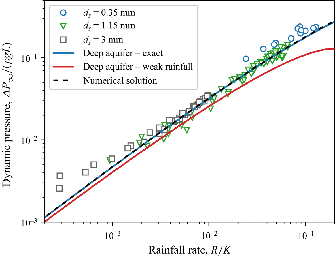
 $R/K$. We find that the three experimental series, obtained with different glass beads, gather along the same curve (figure 10). Moreover, the infinitely deep aquifer theory accounts remarkably well for the experimental pressure, even though the aspect ratio of our experimental aquifer is only
 $a=0.7$ (figure 10). Encouraged by this result, we now turn our attention to the active volume of water stored in the aquifer.
Dimensionless dynamic pressure as a function of the dimensionless rainfall rate. Different markers indicate different experimental series. Blue line: infinitely deep aquifer theory. Red line: weak-rainfall limit of the infinitely deep aquifer theory, (7.7). Dashed black line: numerical computation for an aquifer of aspect ratio  $a=0.7$.

7.3. Active volume
The active volume of water stored in the aquifer during rainfall reads
 \begin{equation} V_a = S L^2 W \int_0^1 {\tilde{h}(\tilde{x})}\,{\rm d}\tilde{x} , \end{equation}
where  $S$ is the porosity of the aquifer. In the absence of an explicit expression for the water table
 $h$, (7.2) is of little practical use. Some algebraic manipulation, however, yields a more convenient expression (Appendix D)
 \begin{equation} \frac{V_a}{S L^2 W} = \frac{1}{1-\tilde{R}}{\rm{Im}}\left[\int_{{free\ surface}} \tilde{z} \,{\rm d}\omega \right] , \end{equation}
which allows us to calculate the active volume of water from the solution of the problem in the mathematical space.
Equation (7.3) holds regardless of the aquifer's aspect ratio. For an infinitely deep one, we replace  $\tilde {z}$ with its expression (7.1) in the above integral, and calculate the result. Figure 9(b) shows a numerical approximation of this expression. As might have been anticipated, the active volume of water stored in the aquifer increases with the rainfall rate, and diverges as the latter approaches the conductivity of the aquifer,
 $R/K \rightarrow 1$. Above this value, the rainfall rate exceeds the infiltration capacity of the aquifer, and overland flow appears, at which point our theory becomes irrelevant.
To compare our experimental data with the deep-aquifer theory, we rescale our volume measurements with respect to the characteristic volume  $S L^2 W$, and plot the result as a function of the dimensionless rainfall rate
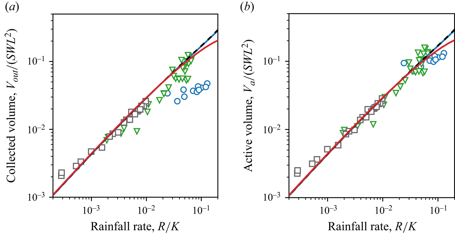
 $R/K$. We find that, unlike pressure, the rescaled volumes do not gather along the same trend, but exhibit a residual dependency on the size of the beads that make up the aquifer (Appendix E, figure 18). We suspect that this trend reflects the influence of capillary effects. In the next section, we discuss this scenario, and propose a crude model that accounts for the proportion of water retained in the aquifer by capillary forces.
7.4. Water retention
We cannot measure directly the active volume of water stored in our experimental aquifer, but we can estimate it from the water collected at its outlet, after the rainfall has stopped. However, as the water table relaxes to its equilibrium shape, a fraction of the water contained in the active volume does not leave the aquifer, but remains trapped in the pores above the water table, due to surface tension (Tschapek, Falasca & Wasowski Reference Tschapek, Falasca and Wasowski1985; De Gennes, Brochard-Wyart & Quéré Reference De Gennes, Brochard-Wyart and Quéré2004; Bear Reference Bear2018). To estimate this fraction, we assimilate the aquifer to a collection of vertical pipes of radius  $r$. The number of pores in a vertical slice of aquifer of length
 $\mathrm {d}\kern 0.06em x$ is thus
 $n = S W\, \mathrm {d}x/({\rm \pi} r^2)$. Assuming that each of them retains a quantity of water proportional to the area of contact with the pore wall, the total volume of water trapped above the outlet reads
 \begin{equation} V_t = \epsilon \int_0^L 2 {\rm \pi}r h \frac{S W \,\mathrm{d} x}{{\rm \pi} r^2} = 2 S \frac{\epsilon}{r} V_a, \end{equation}
where  $\epsilon$ is the thickness of the film of water that remains trapped on the walls of the pores. Estimating the pore size from the aquifer conductivity,
 $d_p=\sqrt {\nu K/g}$, yields the fraction of water that remains trapped in the aquifer
 \begin{equation} \frac{V_t}{V_a} = \frac{2 S \epsilon}{\sqrt{\nu K/g}}, \end{equation}
where  $\nu$ is the kinematic viscosity of water. The above equation allows us to relate the active volume of water to the volume of water collected at the aquifer outlet:
 \begin{equation} V_a = \frac{V_{out}}{1-2 S \epsilon / \sqrt{\nu K/g}} . \end{equation}
Equation (7.6) predicts that the volume of water trapped in the aquifer depends on the characteristic pore size,  $d_p=\sqrt {\nu K/g}$, a result that aligns with the findings of Leverett (Reference Leverett1941).
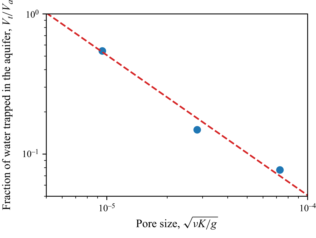
If (7.5) holds, the fraction of water trapped in the aquifer should depend only on pore size. To test this idea, we fill a Darcy column with glass beads, saturate it with water, let it drain and estimate the volume of water trapped in the column by comparing the weight of the column before and after drainage. Figure 11 shows the proportion of water trapped in the Darcy column,  $V_t/V_a$, as a function of pore size,
 $d_p = \sqrt {\nu K/g}$, for the three types of glass beads that make up our experimental aquifer. It varies from almost
 $50\,\%$ for beads of size
 $d_s = 350\,\mathrm {\mu }{\rm m}$ to
 $0.07\,\%$ for beads of size
 $d_s = 3\,{\rm mm}$. A fit of (7.5) consistently reproduces the data, with
 $\epsilon = 6.9\pm 0.2\,\mathrm {\mu }{\rm m}$, a value consistent with previous measurements (Tschapek et al. Reference Tschapek, Falasca and Wasowski1985).
Proportion of water trapped in a Darcy column,  $V_t/V_a$, as a function of the characteristic pore size,
 $d_p = \sqrt {\nu K/g}$. Blue markers: experimental data. Dotted red line: (7.5) with
 $\epsilon$ fitted to the data.

Using this value and (7.6), we evaluate the active volume of water based on the volume collected at the outlet, and plot the result as a function of the rainfall rate (figure 12). The three experimental series, corrected from the effect of surface tension, gather along the same curve, regardless of bead size. Again, the infinitely deep aquifer theory accounts remarkably well for the experimental data. In the next section, we discuss the behaviour of this theory when the rainfall rate is small.
Dimensionless active volume as a function of the dimensionless rainfall rate. The active volume is evaluated from the volume collected at the aquifer's outlet, using (7.6). Different markers indicate different experimental series. Blue line: infinitely deep aquifer theory. Red line: weak-rainfall limit of the infinitely deep aquifer theory (7.8). Dashed black line: numerical computation for an aquifer of aspect ratio  $a=0.7$. Dotted green line: Dupuit–Boussinesq approximation (8.6).

7.5. Weak-rainfall regime
Equation (7.1) provides an exact solution of the flow in an aquifer of infinite depth. We now explore the behaviour of this solution when the rainfall rate is vanishingly small. As the rainfall rate decreases, we expect that the water table will decline until it eventually joins the horizontal axis, when  $\tilde {R}=0$. Expanding (7.1) at leading order in
 $\tilde {R}$, we find (Appendix F):
 \begin{equation} \tilde{\varPhi} \sim \frac{2}{\rm \pi} \tilde{R} \left[ \log\left( \frac{1-{\rm e}^{-{\rm i}{\rm \pi}\tilde{z}}}{\rm \pi}\right) - \log \tilde{R} \right] . \end{equation}
Combining the above equation with the expression of the active volume (7.3) and keeping only the leading terms in  $\tilde {R}$, yields the behaviour of the active volume in the limit of small rainfall rate (Appendix F)
 \begin{equation} \frac{V_a}{ S L^2 W} \sim{-} \frac{2}{\rm \pi} \frac{R}{K} \log \frac{R}{K}. \end{equation}
For a small, but finite, rainfall rate ( $R/K \lesssim 0.1$), the dynamic pressure and the active volume associated with the two approximate expressions above resemble their exact counterpart (figure 9), and provide a good representation of our experimental data (figures 10 and 12).
A surprising feature of (7.7) and (7.8) is that they are nonlinear functions of the rescaled rainfall rate,  $\tilde {R} = R/K$. In other words, the nonlinearity induced by the free surface appears to survive at a vanishingly small rainfall rate. More specifically, the imaginary part of the velocity potential
 $\varPhi$ is proportional to
 $\tilde {R}$, and the shape of the corresponding streamlines remain unaffected by the intensity of the dimensionless rainfall. This is not true, however, for the real part of
 $\varPhi$, that is for the hydraulic head. Anywhere in the aquifer, the hydraulic head is proportional to
 $-\tilde {R}\log \tilde {R}$, at leading order. Even for a vanishingly small rainfall rate, the pressure field in the aquifer thus bears the signature of the nonlinearity induced by the free surface. In the next section, we show that this result can also be derived from the energy balance of the flow.
7.6. Energy balance
To maintain the deformation of the water table, rainfall must inject energy into the aquifer at the constant rate:
 \begin{equation} \mathcal{P} _{in} = \int_0^L \rho g h R W\,{\rm d}\kern0.7pt x =\frac{ \rho g R V_a}{S}. \end{equation}
In steady state and when the outlet barely raises above zero, this energy is entirely dissipated by viscous friction,
 \begin{equation} \mathcal{P} _{d} = W\iint \left(\rho \boldsymbol{g} - {\boldsymbol{\nabla}} p \right) \boldsymbol{q}\,{\rm d}\kern0.7pt x\,{\rm d} y = W \rho g K \iint \left(\boldsymbol{\nabla}\phi\right)^2 \,{\rm d}\kern0.7pt x \,{\rm d} y , \end{equation}
where we integrate over the entire flow. Unfortunately, we were not able to derive a closed-form solution for this integral. Instead, we now perform a scaling analysis to understand how the energy dissipated in the aquifer depends on the parameters of the problem.
We first note that the integrand diverges logarithmically at the outlet. This suggests that most of the energy is dissipated near the outlet, where streamlines get squeezed by the singularity. Accordingly, we replace  $\phi$ with its logarithmic approximation near the outlet (6.11), so that the power dissipated in the aquifer scales as
 \begin{equation} \mathcal{P} _{d} \sim W \rho g K h_s^2 \iint \frac{1}{|z|^2} \,{\rm d}\kern0.7pt x\, {\rm d} y \sim W \rho g K h_s^2 \iint \frac{{\rm d} r}{r} \,{\rm d}\theta, \end{equation}
where we introduce the polar coordinates  $r$ and
 $\theta$. The near-outlet expansion (6.11) is valid at a distance of the outlet longer than a cutoff length which we expect to be about the height of the seepage face,
 $h_s$. Below this distance, the flow interacts with the outlet, and the dissipation saturates. Consequently, we set the lower bound of integral (7.11) to
 $r = h_s$. As for the upper bound, we expect it to scale like the characteristic length of the aquifer
 $r \sim L$. Accordingly, we calculate the integral (7.11) between
 $r = h_s$ and
 $r = L$, and find that
 \begin{equation} \mathcal{P} _{d} \sim{-} W \rho g K h_s^2 \log \frac{h_s}{L}. \end{equation}
We now need to estimate the height of the seepage face,  $h_s$. To do so, we first note that the outlet discharge equilibrates the input rainfall, so that
 $K h_s \boldsymbol {\nabla } \phi \sim RL$. Near the outlet, however, the pressure gradient scales as
 $\boldsymbol {\nabla } \phi \sim h_s/h_s\sim 1$, so that
 $h_s \sim RL/K$, a result consistent with § 6. Replacing the length of the seepage face with the latter expression in (7.12) yields the expression of the viscous dissipation in the aquifer:
 \begin{equation} \mathcal{P} _{d} \sim{-} \frac{W \rho g R^2 L^2}{K} \log \frac{R}{K}. \end{equation}
Equating the input (7.9) and the dissipated (7.13) powers yields the following scaling for the active volume:
 \begin{equation} \frac{V_a}{SWL^2} \sim{-} \frac{R}{K} \log \frac{R}{K}, \end{equation}
which is consistent with (7.8). Because of its simplicity, the above reasoning holds independently of the exact shape of the aquifer outlet, provided it is much smaller than the aquifer itself. We therefore expect that scaling (7.14) applies in situations more general than that of our experiment, provided the rainfall rate is small and the aquifer is deep.
8. Aquifer of finite depth
In the previous section, we discussed the flow in an aquifer of infinite depth, for which there is a closed-form solution. By design, however, the infinitely deep aquifer solution cannot reproduce the shape of the streamlines in our experimental aquifer (figure 5). In this section, we turn our attention towards aquifers of finite depth, and develop a numerical procedure that allows us to compute the flow iteratively. To do this, we first derive an approximate solution for the flow in an aquifer of finite depth recharged by a vanishingly small rainfall rate (§ 8.1). We then use this approximate solution as the initial step of our numerical procedure, with which we finally compute the flow for finite rainfall rates (§ 8.2).
8.1. Approximate solution in the limit of weak rainfall
The mapping (5.13) introduced in § 5.2 simplifies the calculation of the flow by placing the seepage face and the water table on the horizontal axis of the mathematical space (figure 6). Yet, the problem retains a free boundary: the location of the aquifer bottom in the mathematical plane is unknown. In § 7, we bypassed this issue by considering an aquifer of infinite depth. We now use a different limit: we consider an aquifer of finite depth, but send the rainfall rate to zero. In the mathematical plane, this turns the mapping into the identity, which leaves the aquifer's bottom unchanged along the horizontal line  ${\rm Im}(\omega ) = -a$. Based on this observation, we build an approximate solution of the flow by letting the bottom lie at this position (figure 13a). This approximation does not completely eliminate the rainfall rate from the problem, as the latter still determines the length of the seepage face. It does, however, considerably simplify the problem by fixing the shape of the free boundary.
Approximate solution in an aquifer of aspect ratio  $a=0.7$ submitted to a rainfall rate
 $R/K = 0.2$: (a) mathematical plane,
 $\omega = u+{\rm i}v$; and (b) physical plane,
 $\tilde {z} = x/L +{\rm i}y/L$. Laplace's equation is solved within the blue-shaded domain using the finite-element method. Grey triangles: numerical mesh. Orange dashed lines: isoheads. Black dashed lines: streamlines. Here
 $\delta _y$ is the distance between the calculated position of the aquifer's bottom (solid grey line) and its real position in the experiment (dotted black line). The other lines represent the different boundaries of the problem, according to the legend of figure 6.

It is now straightforward to solve the problem numerically. Using pyFreeFem (available at: https://github.com/odevauchelle/pyFreeFem), a Python wrapper for the finite-element software FreeFem++ (Hecht Reference Hecht2012), we solve Laplace's equation, and determine the complex function  $\tilde {z}(\omega )$ that satisfies the boundary conditions in the mathematical plane (figure 13a). We then compute the complex potential from (5.13), and plot the result in the physical space. As expected, our approximate solution looks correct only in the limit of vanishing rainfall rates (
 $\tilde {R}\lesssim 10^{-3}$). As the latter increases, however, the shape of the aquifer bottom deviates from that of the experimental set-up: it curves and rises towards the surface (figure 13b).
To get a better approximation of the flow, we now need to relax the small-rainfall approximation, and return to the original problem. In the next section, we use the weak-rainfall solution as a starting point to develop a better approximation of the flow.
8.2. Relaxation to the nonlinear solution
We now return to the original problem, for which the location of the bottom in the mathematical plane is unknown. To solve it, we develop the following relaxation method. We place ourselves in the weak-rainfall approximation, and compute the corresponding solution, as described in the previous section. In this solution, the shape of the aquifer bottom deviates from the horizontal. It reads  $\tilde {y}_b(\tilde {x}) = -a+\delta _y(\tilde {x})$, where
 $\delta _y(\tilde {x})$ is the deviation of the bottom of the numerical aquifer from the real one: a measure of the numerical error (figure 14a,d).
Convergence to the nonlinear solution in an aquifer of aspect ratio  $a=0.7$ submitted to a rainfall rate
 $R/K = 0.3$. (a) Weak-rainfall approximation, (b) intermediate solution after two iterations and (c) converged solution after 8 iterations in the mathematical plane,
 $\omega = u+{\rm i}v$. (d–f) Corresponding solutions in the physical plane,
 $\tilde {z} = x/L +{\rm i}y/L$. Orange dashed lines: isoheads. Black dashed lines: streamlines. Here
 $\delta _y$ is the distance between the calculated position of the aquifer's bottom (solid grey line) and its real position in the experiment (dotted black line). The other lines represent the different boundaries of the problem, according to the legend of figure 6. The Python routines used to solve that problem are available online: https://github.com/odevauchelle/pyFreeFem.

To reduce this error, we need to deform the mesh in the mathematical plane, so that the bottom in the physical plane moves by an amount opposed to the error,  $-\delta _y(\tilde {x})$. To deform the mesh in the smoothest possible way, we introduce a deformation field,
 $\delta _v$, that satisfies Laplace's equation with the following conditions:
 $$\begin{gather} \delta_v ={-}\delta_y = a+\tilde{y} \quad \text{on the bottom}, \end{gather}$$
 $$\begin{gather}\delta_v = 0 \quad \text{on the seepage face}, \end{gather}$$
 $$\begin{gather}\delta_v = 0 \quad \text{on the water table}, \end{gather}$$
 $$\begin{gather}\partial_n\delta_v = 0 \quad \text{on the divide}, \end{gather}$$
 $$\begin{gather}\partial_n\delta_v = 0 \quad \text{on the wall below the outlet}. \end{gather}$$
The last two boundary conditions are arbitrary. They only need to be compatible with the first one at the junctions with the aquifer's bottom. The reason why we require the deformation field  $\delta \nu$ to satisfy Laplace's equation is not based on any fundamental mathematical principle. Instead, the choice is purely practical: ensuring that
 $\delta \nu$ follows Laplace's equation results in a smooth field, which allows us to deform the mesh in the smoothest possible manner (Hecht et al. Reference Hecht, Pironneau, Le Hyaric and Ohtsuka2005).
Using finite elements, we solve for the deformation field  $\delta _v$, and change the original mesh according to it, replacing
 $v$ with
 $v - \delta _v$. Using, again, finite elements, we solve Laplace's equation and compute
 $\tilde {z}(\omega )$ in this new domain. We then repeat the procedure, in the hope that the shape of the aquifer will converge towards that of the real one (figure 14b,e). We find that, for aspect ratios larger than
 $H/L\gtrsim 10^{-2}$, the above procedure converges to a final mesh in the mathematical plane, which corresponds to a realistic solution in the physical plane: the bottom of the aquifer is almost horizontal, with
 $\tilde {y}_b \approx -a$ (figure 14c,f). Below this limit, the thickness of the aquifer is so small that the deformation of the mesh generates numerical instabilities. We now compare our numerical solutions with our experimental observations.
8.3. Comparison with experiments
The water table and the streamlines computed from our numerical solution appear qualitatively consistent with the experimental observations (figure 14f). To draw a more quantitative comparison, we solve for the flow of groundwater under the experimental conditions of figure 5 ( $R/K = 0.07$,
 $a=0.7$). We find that the numerical seepage face, water table and streamlines fall very close to the experimental observations, without any adjustable parameter (figure 5). Near the outlet, the numerical water table drops a bit below the actual one, and pushes down the streamline. We suspect that this discrepancy is due to surface tension.
Using the numerical procedure of § 8.2, we also compute the pressure and the active volume of water stored in our experimental aquifer, as a function of the rainfall rate. We find that the results are consistent with our experimental data (figures 10 and 12).
Having thus validated our nonlinear theory, we now turn our attention to the dependency of the active volume on the aspect ratio of the aquifer.
8.4. Active volume dependence on aspect ratio
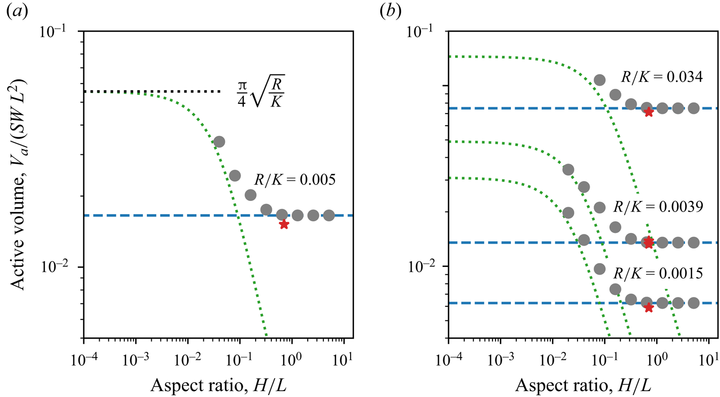
Using the numerical procedure introduced in § 8.2, we compute the active volume of water as a function of the aquifer's aspect ratio for a fixed rainfall rate  $R/K=5\times 10^{-3}$ (figure 15a). Our numerical method converges only for aspect ratios larger than
 $a \gtrsim 10^{-2}$. Within this range, we observe that the active volume decreases as the aquifer becomes deeper (figure 15a). When the aspect ratio exceeds
 $a\sim 0.5$, the active volume of water saturates at the asymptotic value predicted by the infinitely deep aquifer theory (figure 15a).
(a) Active volume of water stored in an aquifer,  $V_a/(SWL^2)$, as a function of its aspect ratio,
 $a=H/L$, for a rainfall rate set to
 $R/K=5\times 10^{-3}$. (b) Relationship between active volume and aspect ratio for three different rainfall rates
 $R/K = 1.5\times 10^{-3}$,
 $3.9\times 10^{-3}$ and
 $3.4\times 10^{-2}$. Grey markers: numerical computation following the procedure described in § 8. Red stars: experimental data. Blue dashed line: infinitely deep aquifer limit (7.1) combined with the integral (7.3). Green dashed line: Dupuit–Boussinesq approximation (8.6).

Repeating this procedure for various rainfall rates reveals the same qualitative behaviour: for a given rainfall rate, the active volume decreases as the aquifer deepens, eventually saturating at a plateau predicted by the infinitely deep aquifer theory (figure 15b). Changing the rainfall rate affects the relation between active volume and aspect ratio in two ways: (1) increasing the rainfall rate shifts this relation towards larger active volumes; and (2) the aspect ratio at which the active volume reaches its plateau slightly increases with the rainfall rate.
Although somewhat counterintuitive, the decrease of the active volume with the aquifer depth is easily understood with the following reasoning. The groundwater discharge roughly scales with the aquifer depth times the velocity of groundwater averaged across the depth of the aquifer. As a result, the deeper the aquifer, the smaller the velocity and, consequently, the smaller the pressure gradient that drives the flow. The deviation of the water surface, which induces this pressure gradient, is therefore smaller in a deeper aquifer.
8.5. Dupuit–Boussinesq approximation
We now compare our numerical computations with the predictions of the Dupuit–Boussinesq approximation. This approximation, which neglects the vertical component of the flow, yields the following prediction for the active volume of water (Appendix G):
 \begin{equation} \frac{V_a}{S L^2 W} = \frac{R/K+a^2}{2\sqrt{R/K}} \arcsin\left(\frac{\sqrt{R/K}}{\sqrt{R/K+a^2} } \right) -\frac{a}{2} . \end{equation}
A comparison of (8.6) with our numerical calculations suggests that the two modelling approaches accord for aspects ratios  $a \lesssim 0.02-0.1$ (figure 15). Unfortunately, our numerical method does not allow us to compute the active volume for aspect ratios smaller than
 $a \lesssim 10^{-2}$. It is therefore impossible to verify whether our numerical calculations approach the Dupuit–Boussinesq prediction of
 $V_a/(S L^2 W) = {\rm \pi}/4 \times \sqrt {R/K}$ as the aspect ratio tends to zero.
For aspect ratios greater than  $a \gtrsim 0.02$–0.1, the Dupuit–Boussinesq approximation systematically underestimates the active volume, a discrepancy that increases with the aquifer's aspect ratio (figure 15). In particular, the Dupuit–Boussinesq approximation predicts that the active volume vanishes when the aspect ratio tends to infinity, whereas it saturates to a finite asymptotic value in the present theory (figure 15). As a result, the Dupuit–Boussinesq approximation utterly fails to predict the active volume in our experimental aquifer of aspect ratio
 $a=0.7$ (figure 12).
A closer look at figure 15(b) suggests that the cutoff aspect ratio, above which the two modelling approaches diverge, slightly varies with the dimensionless rainfall rate  $R/K$. We now discuss this point in more detail. We first note that the flow of groundwater is made of two superimposed horizontal layers (figure 2). The deeper layer, of thickness equal to the aquifer depth
 $H$, lies below the aquifer outlet, and develops a strong vertical flow component near the drainage divide (right wall) and along the vertical wall below the outlet (figure 5). The upper layer lies above the aquifer outlet, and the amplitude of its vertical flow component depends on its thickness, which is equal to the elevation of the water table,
 $h$.
As the Dupuit–Boussinesq approximation requires that the vertical component of the flow be negligible, we suspect that its validity depends on the thickness of the upper layer. If this layer is too thin,  $h \ll H$, the vertical component of the deeper layer dominates the flow, and the Dupuit–Boussinesq approximation fails (figure 16a). Conversely, if the upper layer is too thick compared with the aquifer length,
 $h \gg L$, it develops a strong vertical component, and the Dupuit–Boussinesq approximation fails again (figure 16b). In short, we suspect that the Dupuit–Boussinesq approximation holds only when
 $H \ll h \ll L$ (figure 16c).
Numerical solutions of the flow for different aquifer aspect ratios and rainfall rates: (a)  $a = 1.28$ and
 $R/K=0.001$, (b)
 $a = 0.32$ and
 $R/K=0.5$ and (c)
 $a = 0.08$ and
 $R/K=0.07$. Orange dashed lines: isoheads. Black dashed lines: streamlines. (d) Map of the error of the Dupuit–Boussinesq approximation relative to the present theory in the aspect ratio–rainfall rate plane. The colour and the size of the bullets indicate the amplitude of the relative error. The red dotted line indicates the limits predicted from inequality (8.7). Red stars indicate the position of the solutions (a–c).

Within the Dupuit–Boussinesq approximation, the characteristic thickness of the upper layer scales like  $h/L \sim \sqrt {a^2+R/K} - a$ (Appendix G). The above inequality therefore translate into the following condition:
 \begin{equation} 3 a^2 \ll R/K \ll 1 , \end{equation}
since the rainfall rate cannot exceed  $R/K=1$. To test this prediction, we compare the active volume of water from the Dupuit–Boussinesq approximation (8.6),
 $V_{DB}$, with the prediction of our numerical simulations,
 $V_a$. A map of the relative error between the two models,
 $| V_{db}/V_a - 1|$, in the aspect ratio–rainfall rate plane shows that the Dupuit–Boussinesq approximation works best within the limits predicted by the inequality (8.7) (figure 16d). In short, the Dupuit–Boussinesq approximation is valid provided that the aspect ratio of the aquifer is small, and as long as the rainfall rate is not too low.
9. Conclusion
The experiments presented in this paper have revealed that the active volume of water stored in an aquifer decreases with the depth of the latter. This result conforms with intuition: the discharge at the aquifer outlet scales as the product of its depth by the average flow velocity. In a deeper aquifer, a smaller flow velocity, and consequently a smaller deformation of the water table, is thus required for the groundwater discharge to equilibrate the rainfall input.
Despite its simplicity, turning this qualitative observation into a quantitative prediction proved a challenging problem: the seepage face and the water table freely adjust their shapes to accommodate the rainfall input, and calculating the active volume stored in the aquifer required Darcy's law to be solved inside a domain that is a priori unknown. Four approaches have allowed us to bypass this issue. The first is to linearise the boundary condition at the free surface. This linear theory represents fairly well the flow streamlines in the limit of small rainfall rates ( $R/K \lesssim 5\times 10^{-3}$), but fails to account for the active volume of water stored in the aquifer (Jules et al. Reference Jules, Lajeunesse, Devauchelle, Guérin, Jaupart and Lagrée2021). The second approach is to use the Dupuit–Boussinesq approximation (Horton Reference Horton1936; Guérin et al. Reference Guérin, Devauchelle, Robert, Kitou, Dessert, Quiquerez, Allemand and Lajeunesse2019). By design, this theory, which neglects the vertical component of the groundwater velocity, is unable to represent the flow streamlines (Jules et al. Reference Jules, Lajeunesse, Devauchelle, Guérin, Jaupart and Lagrée2021). However, our numerical calculations show that it provides an accurate estimate of the active volume of water stored in aquifers provided that the aspect ratio of the aquifer is small and the rainfall rate not too low (
 $R/K \gg 3(H/L)^2$). The third approach is to consider the limiting case of an aquifer of infinite depth. In this asymptotic configuration, conformal mapping allows us to map the seepage face and the water table onto well-defined surfaces, and derive a closed-form solution for the groundwater flow. While strictly valid for an aquifer of infinite depth, our experiments and simulations show that this solution provides a satisfying estimate of the active volume provided the aquifer's aspect ratio exceeds
 $H/L\gtrsim 0.5$. We are left with the case of aquifers of aspect ratios between
 $H/L\gtrsim 10^{-2}$ and
 $H/L \lesssim 0.5$, for which we were unable to derive any closed-form solution. Instead, we propose a numerical procedure that allows us to solve the problem. We find that the resulting numerical solution is in good agreement with our experiments.
According to this solution, the active volume in an aquifer, once properly rescaled, is proportional to  $-(R/K)\log (R/K)$. This unusual scaling bears the mark of the viscous dissipation that takes place in the neighbourhood of the river that drains the aquifer. The logarithm of this formula, indeed, is directly inherited from the behaviour of a Darcy flow around a point sink.
As the water table recedes after a rainfall event, surface tension retains a portion of the water stored within the aquifer (Tschapek et al. Reference Tschapek, Falasca and Wasowski1985; De Gennes et al. Reference De Gennes, Brochard-Wyart and Quéré2004). Consequently, the active volume of water stored in the aquifer may be significantly larger than the volume of water collected at the aquifer's outlet, after rainfall has stopped. Based on our experiments, we have proposed a semi-empirical model that accounts for the variation of the fraction of water retained inside the aquifer with the characteristic pore size. Since our experiments involve only water and glass beads, we cannot explore the influence of surface tension. Given that the latter plays a crucial role in the retention process, additional experiments are necessary to elucidate this aspect of the problem.
Our theory predicts that the active volume of water stored in the aquifer depends on two dimensionless parameters: (1) the ratio of the aquifer depth to the aquifer length,  $H/L$; and (2) the ratio of the rainfall rate to the aquifer hydraulic conductivity,
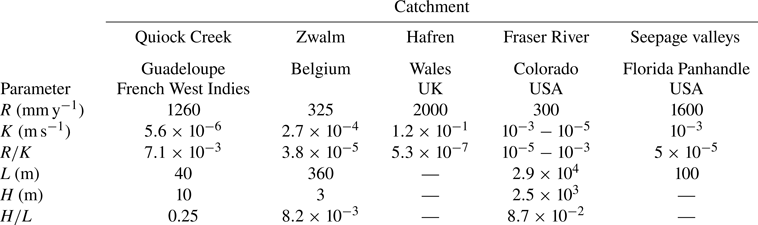
 $R/K$. Evaluating the hydraulic conductivity of an aquifer in the field is notoriously challenging and measuring its depth is even more difficult. As a result, data are scarce. The little we found in the literature fall within the ranges
 $H/L=10^{-3}$ to
 $10^{-1}$ and
 $R/K=10^{-7}$ to
 $10^{-2}$ (Appendix H, table 2). However, these data are likely not representative of the variability of
 $H/L$ and
 $R/K$ in nature. The ongoing development of geophysical methods to map the subsurface of catchments could help to better constrain these two parameters (Pasquet et al. Reference Pasquet, Marçais, Hayes, Sak, Ma and Gaillardet2022).
Annual recharge rate  $R$ (rainfall rate minus evapotranspiration), hydraulic conductivity
 $K$, dimensionless recharge
 $R/K$, aquifer length
 $L$, depth
 $H$ and aspect ratio
 $H/L$ for several aquifers in the field. Data from Pauwels & Troch (Reference Pauwels and Troch2010), Petroff et al. (Reference Petroff, Devauchelle, Abrams, Lobkovsky, Kudrolli and Rothman2011), Aigler & Ge (Reference Aigler and Ge2013), Benettin et al. (Reference Benettin, Kirchner, Rinaldo and Botter2015), Guérin et al. (Reference Guérin, Devauchelle, Robert, Kitou, Dessert, Quiquerez, Allemand and Lajeunesse2019) and Pasquet et al. (Reference Pasquet, Marçais, Hayes, Sak, Ma and Gaillardet2022).

In this paper, we have restricted our analysis to the case of an aquifer bounded by a flat horizontal bottom. However, the iterative numerical scheme presented in § 8.2 can be adapted to accommodate the more complex, variable topographies sometimes encountered in the field (see Appendix I, figure 19).
Finally, our theory has addressed the steady-state regime, for which the discharge at the aquifer outlet balances the rainfall input. As a result, it predicts the maximum volume of water that an aquifer can store (Horton Reference Horton1936). In the field, however, the duration of a rainfall event is often too short for the water table to reach this maximum storage volume. This calls for an investigation of the transient stormflow regime, which is crucial to flood forecasting (Guérin et al. Reference Guérin, Devauchelle, Robert, Kitou, Dessert, Quiquerez, Allemand and Lajeunesse2019). A theory of this dynamical regime remains to be established for deep aquifers.
Acknowledgements
We thank P. Aussillous, P.Y. Lagrée, F. Métivier and J. Neufeld for numerous insightful discussions. We are grateful to O. Bour and S. Pasquet for sharing their expertise about field data. Some of the field data used in this paper were collected by the Observatoire de l'Eau et de l’éRosion aux Antilles (ObsERA, INSU- CNRS, http://webobsera.ipgp.fr/).
Declaration of interests
The authors report no conflict of interest.
Appendix A. Hydraulic conductivity
Figure 17 displays the hydraulic conductivity  $K$ as a function of the characteristic velocity,
 $g d_s^2/\nu$, where
 $d_s$ is the size of the beads that make up the aquifer,
 $\nu$ is the kinematic viscosity of water and
 $g$ is the acceleration of gravity. We find that
 $K$ increases linearly with
 $g d_s^2/\nu$, in accordance with the empirical Kozeni–Carman relationship (Carman Reference Carman1937). A fit of the data yields
 $K = c g d_s^2/\nu$, with
 $c=5.9 \pm 0.1 \times 10^{-4}$.
Hydraulic conductivity,  $K$, as a function of the characteristic velocity,
 $g d_s^2/\nu$, where
 $d_s$ is the size of the beads that make up the aquifer,
 $\nu$ is the kinematic viscosity of water and
 $g$ is the acceleration of gravity. Bullets: experimental data. Red-dotted line: linear relationship fitted to the data.

Appendix B. Flow near the aquifer outlet in the weak-rainfall regime
Near the outlet, the flow is described by the following expression for  $\tilde {z}$,
 \begin{equation} \tilde{z} = \frac{{\rm
i}}{{\rm \pi} (1-\tilde{R} )} [ (\tilde{R} -\omega)
\log(\tilde{R} -\omega) + (\tilde{R} +\omega)
\log(\tilde{R} +\omega) - 2\tilde{R} \log \tilde{R}]
. \end{equation}
To better understand how the seepage face constrains the flow in the aquifer, we expand (B1) under the conditions of a small rainfall rate, and at a distance from the outlet sufficiently large to ensure that  $\tilde {R}/\omega$ is small. Assuming that
 $0 < \tilde {R}/\omega \ll \tilde {R} \ll 1$, we find that
 \begin{equation} \tilde{z} = \omega + \frac{2 {\rm i}}{\rm \pi} \tilde{R} \log\omega , \end{equation}
which yields the following expression for the potential:
 \begin{equation} \tilde{\varPhi} = \frac{2}{\rm \pi} \tilde{R} \log\omega . \end{equation}
As expected when the rainfall rate vanishes, we find  $\tilde {\varPhi } = 0$, and therefore
 $\tilde {z} = \omega$: the water surface is flat, and the groundwater flow vanishes. This observation allows us to further simplify the complex potential and recover (6.10):
 \begin{equation} \tilde{\varPhi} = \frac{2}{\rm \pi} \tilde{R} \log\tilde{z} . \end{equation}
Appendix C. Infinitely deep aquifer
For an infinitely deep aquifer, the condition at the aquifer bottom (5.16) disappears from the set of equations formulated in § 5, and the boundary conditions reduce to
 $$\begin{gather} \tilde{x} = 1 \quad \text{on the divide } (u= 1, v < 0), \end{gather}$$
 $$\begin{gather}\tilde{x} = 0 \quad \text{on the wall below the outlet } (u= 0, v < 0), \end{gather}$$
 $$\begin{gather}\tilde{x} = 0 \quad \text{on the seepage face } (0< u< \tilde{R}, v= 0), \end{gather}$$
 $$\begin{gather}\tilde{x} = \frac{u-\tilde{R}}{1-\tilde{R}} \quad \text{on the water table } (\tilde{R}< u< 1, v= 0). \end{gather}$$
Finding an analytical function  $\tilde {z}(\omega )$ that satisfies these conditions is challenging, due to the dependency of the last boundary condition on the variable
 $u = {\rm Re}(\omega )$. To bypass this issue, we follow a reasoning similar to that of § 6, and look for
 $\tilde {z}'(\omega )$, the derivative of
 $\tilde {z}(\omega )$, instead of
 $\tilde {z}(\omega )$ itself. To do this, we introduce the intermediate function
 $\chi (\omega ) = (1-\tilde {R}) \tilde {z}'$. Both
 $\tilde {z}(\omega )$ and its derivative
 $\tilde {z}'(\omega )$ are analytical, so that our intermediate function
 $\chi (\omega )$ is also analytical. The latter satisfies the following boundary conditions:
 $$\begin{gather} {\rm Im}(\chi)= 0 \quad \text{on the divide}, \end{gather}$$
 $$\begin{gather}{\rm Im}(\chi)= 0 \quad \text{on the wall below the outlet}, \end{gather}$$
 $$\begin{gather}{\rm Re}(\chi)= 0 \quad \text{on the seepage face}, \end{gather}$$
 $$\begin{gather}{\rm Re}(\chi) = 1 \quad \text{on the water table}. \end{gather}$$
This system of equation admits the following solution:
 \begin{equation} \chi ={-} \frac{{\rm i}}{\rm \pi} \log\left( \frac{{\rm e}^{{\rm i}{\rm \pi} \omega} - {\rm e}^{{\rm i}{\rm \pi} \tilde{R}}}{{\rm e}^{{\rm i}{\rm \pi} \omega} - {\rm e}^{-{\rm i}{\rm \pi} \tilde{R}}} \right) + (1-\tilde{R}) . \end{equation}
We now define the integral of  $\chi$ as
 $\tilde {z}_s$:
 \begin{equation} \tilde{z}_s = \int
\frac{\chi}{1-\tilde{R}} \,{\rm d}\omega = \omega +
\frac{1}{{\rm \pi}^2(1-\tilde{R})} [\text{Li}_2( {\rm
e}^{-{\rm i}{\rm \pi} (\omega +\tilde{R})} ) -
\text{Li}_2({\rm e}^{-{\rm i}{\rm \pi} (\omega
-\tilde{R})})],
\end{equation}
where  $\text {Li}_2$ denotes Spence's function. This function, sometimes referred to as ‘dilogarithm’, is defined by the following integral:
 \begin{equation} \text{Li}_2(z) ={-}\int_0^z \frac{\log(1-u)}{u} \,{\rm d}u, \end{equation}
where the logarithm has its branch cut along the real negative axis.
For readability, we have left integral (C10) indefinite. The actual solution of our problem is
 \begin{equation} \tilde{z}(\omega) = \widetilde{z_s}(\omega) - \widetilde{z_s}(0) , \end{equation}
which corresponds to (7.1).
Appendix D. Active volume of water stored in the aquifer during rainfall
The active volume of water stored in the aquifer during rainfall reads
 \begin{equation} V_a = S L^2 W \int_0^1 {\tilde{h}(\tilde{x})} \,{\rm d}\tilde{x} , \end{equation}
where  $S$ is the porosity of the aquifer. To calculate this integral we first note that, at the water table, condition (5.5) allows us to substitute
 $\tilde {\phi }$ for
 $\tilde {h}$ in the above expression. Using the definition of
 $\omega$ (5.13), we also rewrite
 ${\rm d}\tilde {x}$ as
 \begin{equation} {\rm d}\tilde{x} = {\rm d} u - {\rm d}\tilde{\psi}. \end{equation}
Finally, the water balance at the free surface (5.6) yields
 \begin{equation} {\rm d}\tilde{\psi} ={-} \tilde{R} \,{\rm d}\tilde{x}, \end{equation}
so that we can express the active volume in a more convenient way:
 \begin{align} \frac{V_a}{S L^2 W} &= \frac{1}{1-\tilde{R}}~{\rm Re}\left[\int_{{free\ surface}} \tilde{\varPhi}\,{\rm d} u \right]\nonumber\\ &= \frac{1}{1-\tilde{R}}\,{\rm Im}\left[\int_{{free\ surface}} (\tilde{z} - \omega)\,{\rm d} \omega \right] . \end{align}
Integrating the above equation yields (7.3).
Appendix E. Volume of water collected at the aquifer outlet
In our experiments, we evaluate the active volume from the volume of water collected at the aquifer outlet, after the rainfall has stopped. Figure 18(a) displays this volume,  $V_{out}$, rescaled with respect to the characteristic volume
 $S L^2 W$ as a function of the dimensionless rainfall rate,
 $R/K$. The data do not gather along the same trend, but exhibit a residual dependency: the quantity of water collected at the outlet decreases with the size of the beads that make up the aquifer (figure 18a).
(a) Dimensionless volume of water collected at the aquifer outlet as a function of the dimensionless rainfall rate. (b) Dimensionless active volume of water as a function of the dimensionless rainfall rate. The active volume of water is evaluated from the volume collected at the aquifer outlet, using (7.6). Different markers indicate different experimental series (see legend of figure 10). Blue line: infinitely deep aquifer theory. Red line: weak-rainfall limit of the infinitely deep aquifer theory (7.8). Dashed black line: numerical computation for an aquifer of aspect ratio  $a=0.7$.

As discussed in § 7.4, this trend reflects the influence of surface tension, which retains a fraction of the active volume of water stored in the aquifer. Using (7.6), we correct for this effect, and evaluate the active volume of water. We find that the three experimental series, corrected from the effect of surface tension, gather along the same curve, regardless of bead size (figure 18b).
Appendix F. Weak-rainfall regime in an infinitely deep aquifer
Equation (7.1) is an exact solution of Laplace's equation in an aquifer of infinite depth. As the rainfall rate decreases, we expect that the water table declines until it joins the horizontal axis when  $\tilde {R}=0$. Expanding (7.1) at leading order in
 $\tilde {R}$, we find
 \begin{equation} \tilde{\varPhi} \sim \frac{2}{\rm \pi} \tilde{R} [ \log(1-{\rm e}^{-{\rm i}{\rm \pi}\omega}) - \log{\rm \pi} - \log \tilde{R} ] . \end{equation}
As expected when the rainfall rate vanishes, we find  $\tilde {\varPhi } = 0$, and therefore
 $\tilde {z}=\omega$. In short, the water surface is flat and the groundwater flow vanishes. This observation allows us to further simplify the complex potential (F1) by keeping only the leading-order terms. We find
 \begin{equation} \tilde{\varPhi} \sim \frac{2}{\rm \pi} \tilde{R} \left[ \log\left( \frac{1-{\rm e}^{-{\rm i}{\rm \pi}\tilde{z}}}{\rm \pi}\right) - \log \tilde{R} \right] , \end{equation}
which corresponds to (7.7).
To evaluate the active volume of water stored in the aquifer in the limits of small rainfall rates, we inject (F2) in the expression of the active volume (7.3)
 \begin{equation} \frac{V_a}{S L^2 W} \sim \frac{2}{\rm \pi} \tilde{R}\,{\rm Re} \left[ \int_{\tilde{R}}^1 \left[ \log(1-{\rm e}^{-{\rm i}{\rm \pi}\omega}) - \log{\rm \pi} - \log \tilde{R} \right] \,{\rm d}\omega \right], \end{equation}
which, keeping only the leading-order terms in  $\tilde {R}$, yields (7.8):
 \begin{equation} \frac{V_a}{ S L^2 W} \sim{-} \frac{2}{\rm \pi} \tilde{R} \log \tilde{R}. \end{equation}
Appendix G. Active volume in the Dupuit–Boussinesq approximation
The Dupuit–Boussinesq approximation assumes that the vertical component of the flow is negligible with respect to the horizontal one (Dupuit Reference Dupuit1863; Boussinesq Reference Boussinesq1903). Darcy's law (5.1), combined with the mass balance, yields the Dupuit–Boussinesq equation, which, in steady state, reads
 \begin{equation} \frac{\partial^2 (H+h)^2}{\partial x^2} ={-} 2 \frac{R}{K} . \end{equation}
The Dupuit–Boussinesq equation requires two boundary conditions. At the outlet, the groundwater pressure vanishes. The first boundary condition is therefore  $h=0$ in
 $x=0$. The right-hand side of the aquifer is bounded by an impervious wall that mimics a drainage divide. The water discharge therefore vanishes on that wall, a condition that reads
 $\partial h / \partial x=0$ in
 $x=L$. With these two boundary conditions, the Dupuit–Boussinesq equation (G1) admits the following solution (Horton Reference Horton1936):
 \begin{equation} \frac{h}{L} = \sqrt{a^2- \frac{R}{K}\frac{x}{L}\left(\frac{x}{L}-2\right) } - a. \end{equation}
Integrating the above equation yields the expression of the active volume of water stored in the aquifer within the Dupuit–Boussinesq approximation (8.6):
 \begin{equation} \frac{V_a}{S L^2 W} = \frac{R/K+a^2}{2\sqrt{R/K}} \arcsin\left(\frac{\sqrt{R/K}}{\sqrt{R/K+a^2} } \right) -\frac{a}{2} . \end{equation}
This expression appears on figure 15.
When the aspect ratio of the aquifer tends to 0, the active volume predicted from the Dupuit–Boussinesq approximation tends to
 \begin{equation} \frac{V_a}{S L^2 W} = \frac{\rm \pi}{4} \sqrt{R/K} . \end{equation}
Conversely, when the aspect ratio of the aquifer goes to infinity, the active volume tends to  $V_a \sim 0$.
In § 8.5, we define the upper layer of the groundwater flow as the layer of fluid above the outlet level. We estimate the characteristic thickness of this upper layer by setting  $x=L$ in (G2), which yields
 \begin{equation} \frac{h}{L} \sim \sqrt{a^2+\frac{R}{K}} - a . \end{equation}
Appendix H. Aspect ratios and dimensionless recharge rates of free aquifers in nature
The flow of groundwater in a free aquifer depends on two dimensionless parameters: (1) the ratio of the aquifer depth to the aquifer length,  $H/L$; (2) the ratio of the rainfall rate to the aquifer hydraulic conductivity,
 $R/K$. Evaluating the hydraulic conductivity of an aquifer in the field is notoriously challenging and measuring its depth is even more difficult. Table 2 summarises the data we found in the literature. However, this data is likely not representative of the variability of
 $H/L$ and
 $R/K$ in nature.
Appendix I. Tilted aquifer
So far, we have restricted our analysis to the case of an aquifer bounded by a flat horizontal bottom. However, the iterative numerical scheme presented in § 8.2 can be adapted to accommodate the more complex, variable topographies sometimes encountered in the field. Figure 19 shows, for example, the numerical solution obtained in an aquifer inclined with respect to the horizontal. This aquifer of aspect ratio  $a=0.2$ is submitted to a rainfall rate
 $R/K = 0.2$. The slope of its impervious bottom is 0.2 (approximately
 $11\,^{\circ }$). The Python routines used to solve that problem are available online: https://github.com/odevauchelle/pyFreeFem.
Numerical solution in an aquifer inclined with respect to the horizontal: (a) mathematical plane,  $\omega = u+{\rm i}v$; and (b) physical plane,
 $\tilde {z} = x/L +{\rm i}y/L$. The aquifer of aspect ratio
 $a=0.2$ is submitted to a rainfall rate
 $R/K = 0.2$. The slope of its impervious bottom is 0.2. Orange dashed lines: isoheads. Black dashed lines: streamlines. The other lines represent the different boundaries of the problem, according to the legend of figure 6.