Nomenclature

AI

artificial intelligence

ANN

artificial neural network

CART

classification and regression trees

GBDT

gradient boosting decision tree

IoT

Internet of Things

LR

linear regression

LSTM

long short-term memory

LSTM-RNN

long short-term memory recurrent neural network

MAE

mean absolute error

MEMS

micro electro-mechanical systems

MSE

mean square error

NODE

neural ordinary differential equations

PoF

phase of flight

QAR

quick access recorder

RF

random forest

RMSE

root mean square error

SVM

support vector machine

SVR

support vector regression

UAV

unmanned aerial vehicle

XGBoost

Extreme Gradient Boosting

2.0 Machine learning

Machine learning, a sub-branch of artificial intelligence, is the technology of developing computer algorithms that can imitate human intelligence and perform self-learning. It is the modeling of systems, which make predictions by making inferences on data through mathematical and statistical processes, by computers [Reference Mitchell23]. Machine learning algorithms are divided into three categories: supervised, unsupervised and reinforcement learning.

1. i. Supervised learning examines how the relationships between the dependent and the independent variables are learned based on the label information of the data set. Training data consists of both inputs and outputs. If the outputs are categorical, classification algorithms are used, if they are numerical, regression algorithms are used [Reference Kotsiantis, Zaharakis and Pintelas24].

2. ii. Unsupervised learning aims to understand and discover the relationships between unlabeled data. In this type of learning, there is no dependent variable and there is data without a cause and effect relationship. Clustering operations are performed according to the similarities of the observations to each other [Reference Celebi and Aydin25].

3. iii. Reinforcement learning is based on an agent using the trial-and-error method to interact with the environment in a certain situation and complete the given task in the most successful way. Its main purpose is to develop the optimal strategy to obtain the most reward in order to achieve the best result [Reference Sutton26].

The machine learning process, whose flow diagram is given in Fig. 1, is done by performing certain steps. First, data is collected, subjected to preprocessing steps, and received as input. In the preprocessing stage, data cleaning, checking of missing data and taking appropriate actions according to the problem situation are carried out [Reference Alzubi, Nayyar and Kumar27]. Next, model selection and feature engineered steps are applied. It is very important that the model selection is determined with appropriate features depending on the type of problem. Feature engineered is a critical preliminary step for machine learning algorithms. Feature extraction is the process of identifying and removing unnecessary features in order to reduce the problem size and make the algorithms work faster and more effectively. After feature engineered is implemented, the selected model is properly installed. Necessary parameter adjustments of the established model are made to obtain better results. As a result of model training, certain performance evaluation metrics are used to evaluate the performance of the model and model development steps are applied when necessary [Reference Grossberg28–Reference Kuhn, Johnson, Kuhn and Johnson30]. Finally, the predictive values of the model are obtained and the results are analysed. This process can be repeated and continuously improved in machine learning projects [Reference Farhat, Mourali, Jemni and Ezzedine31].

Figure 1.

Flow diagram of the machine learning process.

The types of machine learning algorithm preferred in this study are briefly explained below.

2.1 Linear regression

Linear regression (LR) is a supervised learning algorithm that determines how the dependent variable constantly changes according to a set of independent variables and the relationship between them [Reference Liang and Song32]. The widely used linear regression is generally preferred in small data sets thanks to its simple structure. The parameters of the model can be easily interpreted. This makes it easier for analysts to understand the relationships between variables and explain the outputs of the model [Reference Su, Yan and Tsai33]. The mathematical model of simple LR is given in Equation (1) [Reference Fitzmaurice34].

(1) \begin{align}{y_i} = {\beta _0} + {\beta _1}\,{x_i} + {e_i}\end{align}

Here, n is the number of individuals (i = 1, …,n), y _i is the dependent variable, x _i is the independent variable, e _i is a random error term representing uncertainties, and $\beta_{\textit{0}}$ and $\beta_{\textit{1}}$ are the regression coefficients [Reference Fitzmaurice34].

2.2 Support vector regression

Support vector machines (SVM) consist of two basic categories as classification and solving regression problems. The basic working principle is to perform classification or regression operations on data points by creating a hyperplane [Reference Aghelpour, Mohammadi and Biazar35, Reference Cortes and Vapnik36].

SVM used in regression problems are called as support vector regression (SVR). SVR is a supervised learning model that aims to achieve good performance on both linear and nonlinear data sets. SVR tries to learn an optimal hyperplane with the most points within a margin using support vectors representing the closest data points on the hyperplane. This margin provides an organisation that is increasing the generalisation ability of the model [Reference Awad, Khanna, Awad and Khanna37].

The relationship between input and output in SVR is formulated with a linear function as given in Equation (2) [Reference Deka38].

(2) \begin{align}f\left( x \right) = {w^T}\phi \left( x \right) + b\end{align}

Here, f(x) is the predicted value, w is the weight vector, and φ(x) is the kernel function. Various kernel functions such as linear, polynomial, radial basis function and sigmoid, which form the basis of SVR, can be selected depending on the problem and data set and are used to move the data to a high-dimensional feature space [Reference Cortez and Morais39]. b is the bias value and provides the effect that determines how the classes will be separated.

2.4 Random forest regression

Random forest (RF) is an ensemble learning method that works by combining many decision trees for classification and regression operations. It aims to create a general and effective model by combining different learning algorithms. RF regression combines the predictions of decision trees and uses the voting method for classification problems and the mean value for regression problems [Reference Breiman44, Reference Breiman45]. The basic working principle of the RF algorithm is given in Equation (3).

(3) \begin{align}\hat y = {1 \over n}\mathop \sum \limits_{1 = i}^1 {h_i}\left( x \right)\end{align}

Here, ŷ is the general estimate, n is the total number of trees, h _i is the estimated value of the decision tree, and x is the mean of the independent variables [Reference Cutler, Cutler and Stevens46].

In RF regression, decision trees are combined into a hierarchical structure. This arrangement, which prevents the over-learning problem of a single tree structure, ensures that each tree has a hierarchical structure. Each tree represents the applied constraints, starting from a root node. The diversity between the trees reduces the tendency of the model to over-learning, allowing it to make more general and reliable predictions [Reference Breiman42, Reference Cox47, Reference Quinlan48].

The advantages of RF include working effectively on complex data sets, being resistant to over-learning and outliers. It is used to obtain successful results especially on large and complex data sets [Reference Kotsiantis, Zaharakis and Pintelas24]. These features make RF stand out as a machine learning method with wide application areas.

2.5 Extreme Gradient Boosting

Extreme Gradient Boosting (XGBoost) is a decision tree-based ensemble machine learning algorithm. Gradient boosting decision tree (GBDT) algorithm is a XGBoost version developed to increase speed and prediction performance. It performs well in both classification and regression problems. The XGBoost algorithm uses a mathematical function expressed as the sum of the predictions (ŷ _i) of the total k trees in an ensemble, as given in Equation (4). In this function, the prediction of each tree for observation number i is represented by f _k (x _i ) [Reference Chen and Guestrin49].

(4) \begin{align}{\hat y_i} = \mathop \sum \limits_{k = 1}^k {f_k}\left( {{x_i}} \right),{f_k} \in F\end{align}

The main purpose of the algorithm is to improve the tree created from continuously splitting trees according to the residual error between the prediction results of the previous one and the true value. The new prediction value is obtained by adding it to the previous prediction value [Reference Chen and Guestrin49, Reference Li, An, Li, Wang, Yu, Zhou and Geng50]. As a result, the trees are connected to each other and a tree tries to correct the residual errors of the predictions of the previous trees.

3.0 Problem definition

In this section, the steps followed for takeoff speed prediction using machine learning algorithms and the proposed models are discussed.

First, the data set was determined. For this purpose, the aircraft takeoff data shared by Boeing was used. This data set consists of the pressure altitude in feet (ft) during aircraft takeoff, the outer environmental temperature in Fahrenheit (F), the aircraft’s weight in pounds (lb), the angle of the flaps on its wings in degrees (°) and the aircraft’s speed in knots (kn). The lower and upper limits given in the data set for these variables are 0-9000 ft for pressure altitude, (-40)-(160) F for temperature, 75–140lb for weight, 1°–15° for flap angle, and 98–162kn for takeoff speed, respectively [22].

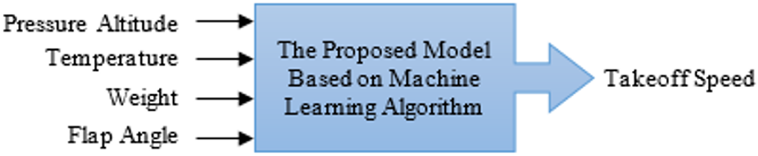
In the model proposed in this study, the pressure altitude, the outer environmental temperature, aircraft’s weight and flap angle were selected as independent variables, and the takeoff speed was selected as the dependent variable. Analytical methods are not very suitable for takeoff speed prediction using this complex relationship consisting of independent-dependent variables. For this reason, artificial intelligence techniques are used to solve problems with complex relationships that do not have a direct relationship between them. In this study, machine learning, one of the artificial intelligence techniques, was preferred in the takeoff speed prediction with complex relationships. The block diagram of the proposed method is presented in Fig. 2.

Figure 2.

Block diagram of the proposed models for takeoff speed prediction.

After determining the data, LR, SVR, CART, RF and XGBoost algorithms were selected from machine learning algorithms for training and test the data. Seventy per cent of the data set was used for training and 30% for testing, and the models were created accordingly. These algorithms were modeled using Anaconda Python software.

The root mean square error (RMSE) expressed by Equation (5), the mean square error (MSE) expressed by Equation (6) and the mean absolute error (MAE) expressed by Equation (7) were used as performance criteria to evaluate the simulation performance. The smaller the error value, the higher the model accuracy is considered. Therefore, these metrics were prefered to objectively evaluate the performance of the proposed models [Reference Chicco, Warrens and Jurman51].

(5) \begin{align}RMSE = \sqrt {{1 \over n}\mathop \sum \limits_{i = 1}^n {{\left( {{y_i} - {{\hat y}_i}} \right)}^2}} \end{align}

(6) \begin{align}MSE = {1 \over n}\mathop \sum \limits_{i = 1}^n {\left( {{y_i} - \hat yi} \right)^2}\end{align}

(7) \begin{align}MAE = {1 \over n}\mathop \sum \limits_{i = 1}^n \left| {{y_i} - {{\hat y}_i}} \right|\end{align}

4.0 Simulation results

In this section, the results of the study are presented in detail.

The first step of the study is to determine the data. For this purpose, the aircraft takeoff data shared by Boeing was used. The parameters of pressure altitude, the outer environment temperature, aircraft’s weight, the angle of the flaps were selected as independent variables and takeoff speed was selected as dependent variable. Then, the data pre-processing step was performed. In this step, missing values, outliers and variable types were checked and necessary corrections were made. The StandardScaler operation in the Scikit-Learn library was applied to scale the data. Thus, each variable was standardised. The standardised data was separated as 70% train data and 30% test data with the holdout method. Models were generated using LR, SVR, CART, RF and XGBoost algorithms from machine learning algorithms. The generated models were trained with the training data and evaluated with the test data. For takeoff speed estimation, the values of the performance criteria of the simulation results made with base models are presented in Table 1.

Table 1.

The RMSE, MSE and MAE values of the proposed base models

When Table 1 is examined, the largest error metric value is obtained in the SVR model, while the smallest error metric value is obtained in the XGBoost model. Considering the error values of the proposed base models to improve the performance of the selected models, feature engineered steps were applied and new variables were added. The new variables derived in this study represent important factors that evaluate the performance of the aircraft. Speed_weight_ratio measures agility of the aircraft by showing the ratio of speed to weight. Altitude_flaps_ratio evaluates the relationship between pressure altitudes and flaps. Performance_score measures overall performance by considering the interaction between speed, weight and flaps. Altitude_pressure reflects the interaction between pressure altitude and temperature. Flap_weight_ratio affects manoeuverability by determining the ratio of flaps to weight. These characteristics help understand the aircraft’s efficiency. The correlation map of the numerical data created with these new variables is presented in Fig. 3.

Figure 3.

The correlation map of the numerical data created with these new variables.

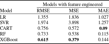
When the correlation map of the numerical data in Fig. 3 is examined, since the flap angle is a categorical variable, it is not directly specified in the correlation map. However, new variables were generated using the flap angle data. Remodelings and predictions were made using the updated data set with the addition of new variables. For this purpose, scaling was first applied to the updated data. Then, the scaled data was separated into training and test data at the same rates in the base model using the holdout method. Models were generated again using LR, SVR, CART, RF and XGBoost algorithms. The new models generated were trained with training data and evaluated with test data. For takeoff speed prediction, the RMSE, MSE and MAE values of the simulation results made with the new models obtained by applying feature engineered are presented in Table 2.

Table 2.

The RMSE, MSE and MAE values of the proposed new models with feature engineered

When Table 2 is examined, in the takeoff speed prediction made with the new feature engineered models, the largest error metric value is obtained in the SVR model, while the smallest error metric value is obtained in the XGBoost model. Although there is a minimal increase in the error values in the feature engineered model compared to the base model for XGBoost, when Table 2 is compared to Table 1, it is generally seen that there is an improvement in the error values of the proposed models. In other words, it is seen that the models generated with the feature engineered data perform better than the base models. The comparison of the actual takeoff speed values and the takeoff speed values estimated with models established with the feature engineered data is given from Figs. 4 to 8, respectively, for the LR, SVR, CART, RF and XGBoost algorithms.

Figure 4.

Comparison of actual takeoff speed values with predicted takeoff speed values for LR.

Figure 5.

Comparison of actual takeoff speed values with predicted takeoff speed values for SVR.

Figure 6.

Comparison of actual takeoff speed values with predicted takeoff speed values for CART.

Figure 7.

Comparison of actual takeoff speed values with predicted takeoff speed values for RF.

Figure 8.

Comparison of actual takeoff speed values with predicted takeoff speed values for XGBoost.

The comparison of the true takeoff speed values with the predicted takeoff speed values is presented in the first column (A) of Fig. 9. The graphs of true versus predicted values make it easier to visually evaluate the model accuracy and variability with the regression line and 95% confidence interval. The graphs of the residuals versus predicted values in the second column (B) of Fig. 9 analyse the distribution of errors in the model predictions. In these graphs, the red line representing zero error provides a reference for evaulating the accuracy of the predictions.

Figure 9.

First column A: Comparison of actual takeoff speed values with predicted takeoff speed values, second column B: Comparison of the residuals versus predicted values, for LR, CART, RF, SVR and XGBoost algorithms.

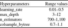
When the figures comparing the actual takeoff speed values with the estimated takeoff speed values are examined, satisfactory results are observed. However, another method that can be done to increase the model performance is hyperparameter optimisation. In this study, when Table 2 is taken as reference, it is seen that the XGBoost algorithm has a smaller error value compared to the other models. Therefore, hyperparameter optimisation was applied to the XGBoost algorithm to increase the model performance. For this purpose, learning_rate, max_depth, n_estimators, colsample_bytree hyperparameters were selected for optimisation. learning_rate limits the contribution of each tree and its default value is 0.3. max_depth controls the maximum depth of the trees and its default value is 6. n_estimators affects the complexity of the model and its default value is 100. colsample_bytree determines the percentage of random selection of features for each tree and its default value is 1. The value ranges selected for hyperparameter optimisation in this study are given in Table 3.

Using GridSearchCV, hyperparameter optimisation on the XGBoost model was performed with using the value ranges in Table 3. he optimisation result was obtained as learning_rate=0.05, max_depth=6, n_estimators=1000, colsample_bytree=1. As a result of the simulation performed with the new XGBoost model established with the obtained optimum hyperparameter values, the RMSE value was found as 0.564, the MSE value as 0.319 and the MAE value as 0.143. The comparison of the actual takeoff speed values and the takeoff speed values estimated with the new XGBoost model is given in Fig. 10.

When Fig. 10 is examined, it is seen that the XGBoost algorithm shows better performance in takeoff speed prediction than previous models with the determined hyperparameters.