2. A calendar year model

Let us denote by $\tau_{t,x}$ , the random remaining lifetime of a x years old individual at time t. We assume that the death occurs when then integral of mortality rates reaches the realization of an exponential random variable $\epsilon$ , of parameter 1. Mortality processes are denoted by $\left(\mu_{t,x}\right)_{t\geq0,x\geq0}$ where $t\,\geq\,0$ is the calendar time and $x\in[0,\omega]$ is the age. 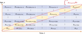They are defined on a probability space $\Omega$ , endowed with their filtration $\left(\mathcal{G}_{t}\right)_{t\geq0}$ and a probability measure P. Contrary to existing affine frameworks, we consider a continuum of mortality processes for each age x instead of a single mortality process per cohort. The set of mortality rates is then a random field indexed by time and age, as illustrated in Figure 1.

Figure 1.

Mortality rates belong to a random field indexed by time and age. The survival probability $P\!\left(\tau_{t,x}\geq s\,|\,\mathcal{G}_{s}\right)$ depends then on a continuum of random variables $\left(\mu_{t+u,x+u}\right)_{u\in[0,s-t]}$ .

In this model, the probability that the individual survives up to time s, conditionally to the knowledge of $\,\left(\mu_{t+u,x+u}\right)_{u\in[0,s-t]}$ , is then equal to

(2.1) \begin{eqnarray}P\!\left(\tau_{t,x}\geq s-t\,|\,\mathcal{G}_{s}\right) & = & P\!\left(\int_{0}^{s-t}\mu_{t+u,x+u}du\geq\epsilon\right)\\[5pt] & = & \exp\!\left(-\int_{0}^{s-t}\mu_{t+u,x+u}du\right)\,.\nonumber\end{eqnarray}

The integral in this last expression is an integral of an infinity of processes indexed by $x+u$ for $u\in[0,s-t]$ as illustrated in Figure 1.

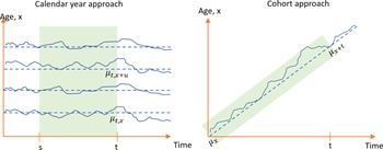
Our model is a calendar year approach in the sense that we associate with each age x, a mortality process indexed by the calendar time. In an affine framework such as the one of Luciano and Vigna (Reference Luciano and Vigna2005), mortality rates are defined by cohort and the survival probability depends on a single mortality process indexed by the cohort age. Figure 2 compares the calendar year and the cohort approaches. Cohort models usually present a high level of analytical tractability and offer closed-form expression for survival probabilities. Nevertheless, their calibration requires to observe the mortality of cohorts till their extinction. For this exercise, we have then to consider mortality rates dating from the first half of the 19th century. This introduces a bias in the estimation due to the considerable progress made in the healthcare sector during the last 50 years. An alternative to estimate affine cohort models consists in fitting them to prospective tables computed with a statistical method. Nevertheless, this approach lacks of consistency and accumulates biases from the cohort model and from the statistical method used for the construction of prospective tables. Another issue is the joint-modeling of multiple cohorts. A life insurer is exposed to mortality/longevity risks of customers belonging to different cohorts. Introducing correlations between cohorts is a challenging task which reduces the analytical tractability of cohort models. From a statistical inference point of view, a calendar year approach is more reliable as it is based on multiple time series of mortality rates. These time series are stationary, and the calendar year model can be estimated with data on a smaller time window than a cohort model. In the remainder of this article, we show that it is still possible to infer analytical expression for survival probabilities subject to some assumptions on the evolution of mortality. By construction, the correlation between cohorts is included in the calendar year approach.

Figure 2.

Comparison of calendar year and cohort approaches. Shaded areas represent the time window of data needed for statistical inference.

In our framework, the death occurs when then integral of mortality processes reaches the realization of an exponential random variable of parameter 1. An alternative approach consists in assuming that the death occurs at the first jump of a point process. But the alternative definition (2.1) allows us to consider mortality processes $\left(\mu_{t,x}\right)_{t\geq0}$ defined on $\mathbb{R}$ instead of $\mathbb{R}^{+}$ . This feature makes then possible to adopt a Gaussian model for $\left(\mu_{t,x}\right)_{t\geq0}$ leading to closed-form expression of survival probabilities. Notice that Gaussian frameworks are also used for approximating the dynamic of mortality rates in various affine cohort models, as in Luciano and Vigna (Reference Luciano and Vigna2005) or Zeddouk and Devolder (Reference Zeddouk and Devolder2020).

In order to preserve the analytical tractability of further developments, we assume that mortality processes are Gaussian with a mean-reverting dynamic defined by:

(2.2) \begin{equation}d\mu_{t,x}=\kappa\!\left(\theta_{t}\,\mu(x)-\mu_{t,x}\right)dt+\Sigma(x)^{\top}d\boldsymbol{W}_{t}^{\mu}\,,\end{equation}

where $\kappa\in\mathbb{R}^{+}$ and $\left(\boldsymbol{W}_{t}^{\mu}\right)_{t\geq0}\in\mathbb{R}^{d}$ is a Brownian motion of dimension d, common to all $\left(\mu_{t,x}\right)_{x\in[0,\omega]}$ . $\left(\theta_{t}\right)_{t\geq0}$ is a stochastic process driving the evolution of longevity. $\Sigma(x)=\left(\Sigma_{1}(x),...,\Sigma_{d}(x)\right)$ is a volatility vector where, $\Sigma_{k}(x)\;:\;[0,\omega]\to\mathbb{R}^{+}$ is a continuous function of age for $k=1,...,d$ . The mean reversion level of $\mu_{t,x}$ is the product of the longevity process $\left(\theta_{t}\right)_{t\geq0}$ and of a continuous function $\mu(x)\;:\;[0,\omega]\to\mathbb{R}^{+}$ , defining the baseline mortality. This function can be the Gompertz–Makeham law or any other parametric function. The longevity process is a mean-reverting jump-diffusion defined by:

(2.3) \begin{equation}d\theta_{t}=\alpha\!\left(\beta(t)-\theta_{t}\right)dt+\nu dW_{t}^{\theta}+dL_{t}\,,\end{equation}

where $\alpha\in\mathbb{R}^{+}$ and $\left(W_{t}^{\theta}\right)_{t\geq0}$ is a Brownian motion independent of $\left(\boldsymbol{W}_{t}^{\mu}\right)_{t\geq0}$ . The function $\beta(t)\;:\;\mathbb{R}^{+}\to\mathbb{R}^{+}$ is strictly positive and decreasing. In later developments, we assume that $\beta(t)$ is equal to

\begin{eqnarray*}\beta(t) & = & \theta_{0}e^{-\gamma t}+\bar{\theta}\!\left(1-e^{-\gamma t}\right)\,,\end{eqnarray*}

where $\theta_{0}$ , $\bar{\theta}$ , and $\gamma\in\mathbb{R}^{+}$ . For this choice of $\beta(t)$ , $\theta_{t}$ converges on average to $\bar{\theta}$ that is lower than $\theta_{0}$ . In order to replicate jumps in mortality caused by pandemics such as the one of COVID-19, we assume that the longevity risk process is exposed to positive jumps. The jump size, denoted by J, is distributed according to an exponential distribution of parameter $\rho$ . The moment generating function of jumps is denoted by:

\begin{align*}\psi(\omega) & =\mathbb{E}\!\left(e^{\omega J}\right)=\frac{\rho}{\rho-\omega},\omega<\rho.\end{align*}

Shocks hitting the longevity process, occur according to a Poisson process, denoted by $\left(N_{t}\right)_{t\geq0}$ , with an intensity $\lambda$ and such that

\begin{align*} L_{t}=\sum_{k=1}^{N_{t}}J_{k}\,.\end{align*}

The filtration of $\left(\theta_{t}\right)_{t\geq0}$ is denoted by $\mathcal{H}_{t}$ . The union of mortality and longevity filtrations is $\mathcal{F}_{t}=\mathcal{G}_{t}\vee\mathcal{H}_{t}$ . Notice that we could think to introduce correlation between longevity and mortality processes. Nevertheless, given the additive structure of $\mu_{t,x}$ and as $\left(\theta_{t}\right)_{t\geq0}$ is not directly observed, this correlation cannot be estimated. Contrary to an affine framework in which there is one single mortality rate process per cohort, the calculation of survival probabilities involves an infinity of mortality processes. Nevertheless, the next section shows that it is still possible to infer closed-form expression for these probabilities.

3. Survival probabilities

Over the last 20 years, statistical frameworks based on the LC model (Reference Lee and Carter1992) became a standard in the insurance industry. This success is explained by several features such as their statistical robustness and their ability to explain the evolution of longevity. Their main disadvantage is that survival probabilities do not admit analytical solution and need to be computed by Monte-Carlo simulations.

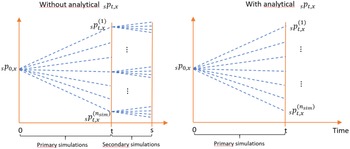
In the context of Solvency II, estimating the SCR and the risk margin (RM) for covering adverse evolution of longevity is therefore computationally intensive. For instance, to forecast future SCR’s covering the longevity risk of a portfolio of annuities, we have to consider simulations in simulations (eventually approached by the Longstaff–Schwartz method) to calculate survival probabilities. Figure 3 illustrates this point. Let us imagine that we generate $n_{sim}$ primary scenarios of mortality and evaluate survival probabilities, noted $\left(_{s}p^{(k)}{}_{t,x}\right)_{k=1,...,n_{sim}}$ in each simulation. In the absence of analytical formula, we have to simulate for each primary scenario several secondary mortality paths up to time s to estimate $_{s}p^{(k)}{}_{t,x}$ . This is done by computing by the following average:

\begin{eqnarray*}\,_{s}p_{t,x}^{(k)} & = & \mathbb{E}\!\left(e^{-\int_{0}^{s-t}\mu_{t+u,x+u}du}\,|\,\mathcal{F}_{t}\right)\\[5pt] & \approx & \frac{1}{n_{sec.\,sim.}}\sum_{j=1}^{n_{sec.\,sim.}}\left(\!\exp\!\left(-\sum_{u=0}^{s-t-1}\mu_{t+u,x+u}^{(k,j)}\right)\right)\,,\end{eqnarray*}

where $n_{sec.\,sim.}$ is the number of secondary simulations and $\mu_{t+u,x+u}^{(k,j)}$ is the simulated mortality force in the $j{\rm th}$ secondary scenario of the $k{\rm th}$ primary scenario (i.e., $\mu_{t,x}^{(k,j)}=\mu_{t,x}^{(k)}$ ). We will see that the calendar year model studied in this article admits analytical expressions for survival probabilities and then remedies to this drawback. By construction, conditionally to the sample paths of $\,\left(\mu_{t+u,x+u}\right)_{u\in[s,t]}$ , the survival probability is provided by Equation (2.1). The unconditional survival probability of a x-year-old individual at time t up to time s noted $_{s}p_{t,x}$ is therefore equal to an expectation:

\begin{eqnarray*} _{s}p_{t,x}&=&P\!\left(\tau_{t,x}\geq s\right)\\[5pt] &=& \mathbb{E}\!\left(\!\exp\!\left(-\int_{0}^{s-t}\mu_{t+u,x+u}du\right)\,|\,\mathcal{F}_{t}\right)\,.\end{eqnarray*}

Figure 3.

Analytical framework versus simulations in simulations.

In order to calculate this expectation, we first develop the analytical expression of $\mu_{t+u,x+u}$ conditioned by $\mathcal{F}_{t}$ , as stated in the next proposition.

Proposition 3.1. For $u\in[0,\omega-x]$ , the mortality process $\mu_{t+u,x+u}$ may be developed as follows:

(3.1)

where , $\tilde{W}_{z}^{\theta}=W_{t+z}^{\theta}$ are Brownian motions and $\tilde{L}_{z}=L_{t+z}$ is a compound Poisson process.

A key quantity for calculating the survival probability is the integral of $\mu_{t+u,x+u}$ . The next proposition states that is may be rewritten as the sum of a deterministic drift, several Brownian integrals, and a jump component. This result will next be used to infer survival probabilities.

Proposition 3.2. For any $\xi\geq0$ , the integral $\int_{0}^{\xi}\mu_{t+u,x+u}du$ may be developed as follows:

(3.2)

We dispose of all the elements to propose a closed-form expression of the survival probability.

Proposition 3.3. The survival probability of a x-year-old individual at time t up to time s, noted $_{s}p_{t,x}$ , is equal to

(3.3) \begin{eqnarray}_{s}p_{t,x} & = & \exp\!\left(-\,_{s-t}m_{t,x}+\frac{1}{2}\,_{s-t}v_{t,x}+A(0,s-t)\right)\end{eqnarray}

where $_{\xi}m_{t,x}$ is drift of the integral $\int_{0}^{\xi}\mu_{t+u,x+u}du$ , that is

(3.4) \begin{eqnarray}\,_{\xi}m_{t,x} & = & \int_{0}^{\xi}e^{-\kappa u}\mu_{t,x+u}du+\frac{\kappa\theta_{t}}{\kappa-\alpha}\int_{0}^{\xi}\mu(x+u)\left(e^{-\alpha u}-e^{-\kappa u}\right)du\\[5pt] & & +\frac{\kappa\alpha\!\left(\theta_{0}-\bar{\theta}\right)e^{-\gamma t}}{\kappa-\alpha}\int_{0}^{\xi}\mu(x+u)\left(\frac{e^{-\gamma u}-e^{-\alpha u}}{\alpha-\gamma}-\frac{e^{-\gamma u}-e^{-\kappa u}}{\kappa-\gamma}\right)du\nonumber \\[5pt] & & +\frac{\kappa\alpha\bar{\theta}}{\kappa-\alpha}\int_{0}^{\xi}\mu(x+u)\left(\frac{1}{\alpha}\left(1-e^{-\alpha u}\right)-\frac{1}{\kappa}\left(1-e^{-\kappa u}\right)\right)du\,.\nonumber\end{eqnarray}

and $\,_{\xi}v_{t,x}$ is the variance of the Brownian part of $\int_{0}^{\xi}\mu_{t+u,x+u}du$ :

(3.5) \begin{eqnarray}\,_{\xi}v_{t,x} & = & \left(\frac{\kappa\nu}{\kappa-\alpha}\right)^{2}\int_{0}^{\xi}\left(\int_{z}^{\xi}\mu(x+u)\left(e^{-\alpha(u-z)}-e^{-\kappa(u-z)}\right)du\right)^{2}\,dz\\[5pt] & & +\int_{0}^{\xi}\left(\int_{z}^{\xi}\Sigma(x+u)e^{-\kappa(u-z)}du\right)^{\top}\left(\int_{z}^{\xi}\Sigma(x+u)e^{-\kappa(u-z)}du\right)dz\,.\nonumber\end{eqnarray}

Whereas the function $A(\xi,s-t)$ solves the following ordinary differential equation (ODE):

(3.6) \begin{eqnarray} \partial_{\xi}A(\xi,s-t) = -\lambda\!\left(\psi\!\left(-\frac{\kappa}{\kappa-\alpha}\int_{\xi}^{s-t}\mu(x+v)\left(e^{-\alpha(v-\xi)}-e^{-\kappa(v-\xi)}\right)\,dv\right)-1\right),\end{eqnarray}

with the terminal condition $A(s-t,s-t)=0$ .

For general expressions of $\mu(x)$ and $\Sigma(x)$ , the integrals in Equations (3.4), (3.5), and (3.6) are numerically computable. The ODE (3.6) is also solved numerically by finite difference approximation. For some model specifications, they can be fully developed. For instance, this is the case when $\mu(x)$ follows a Gompertz–Makeham distribution:

(3.7) \begin{eqnarray}\mu(x) & = & a+bc^{x}\,,\end{eqnarray}

where $a\in\mathbb{R}^{+}$ is the constant death rate caused by accidents and $bc^{x}$ with $b,c\in\mathbb{R}^{+}$ is proportional to age. We will see in numerical illustrations that this assumption provides a good fit to mortality tables with a parsimonious model.

Corollary 3.4. If the function $\mu(x)$ defining the level of mean reversion of mortality rates is the Gompertz–Makeham law (3.7), the drift $\,_{\xi}m_{t,x}$ of $\int_{0}^{\xi}\mu_{t+u,x+u}du$ , is

(3.8) \begin{eqnarray} \,_{\xi}m_{t,x}&=&\int_{0}^{\xi}e^{-\kappa u}\mu_{t,x+u}du+\frac{\kappa\theta_{t}}{\kappa-\alpha}\left(\frac{a}{\alpha}\left(1-e^{-\alpha\xi}\right)-\frac{a}{\kappa}\left(1-e^{-\kappa\xi}\right)\right)\\[5pt] & & +\frac{\kappa\theta_{t}}{\kappa-\alpha}\left(\frac{bc^{x}\left(e^{\left(\ln c-\alpha\right)\xi}-1\right)}{\ln c-\alpha}-\frac{bc^{x}\left(e^{\left(\ln c-\kappa\right)\xi}-1\right)}{\ln c-\kappa}\right)\nonumber \\[5pt] & & +\frac{\kappa\alpha\!\left(\theta_{0}-\bar{\theta}\right)e^{-\gamma t}\left(\frac{1}{\alpha-\gamma}-\frac{1}{\kappa-\gamma}\right)}{\kappa-\alpha}\left(\frac{a}{\gamma}\left(1-e^{-\epsilon\gamma}\right)-\frac{a}{\alpha}\left(1-e^{-\alpha\xi}\right)\right)\nonumber \\[5pt] & & +\frac{\kappa\alpha\!\left(\theta_{0}-\bar{\theta}\right)e^{-\gamma t}\left(\frac{1}{\alpha-\gamma}-\frac{1}{\kappa-\gamma}\right)}{\kappa-\alpha}\left(\frac{bc^{x}\left(e^{\left(\ln c-\gamma\right)\xi}-1\right)}{\ln c-\gamma}-\frac{bc^{x}\left(e^{\left(\ln c-\alpha\right)\xi}-1\right)}{\ln c-\alpha}\right)\nonumber \\[5pt] & & +\frac{\kappa\alpha\bar{\theta}}{\kappa-\alpha}\left(\frac{1}{\alpha}-\frac{1}{\kappa}\right)\left(a\xi+\frac{bc^{x}\left(e^{\xi\ln c}-1\right)}{\ln c}\right)\nonumber \\[5pt] & & +\frac{\kappa\alpha\bar{\theta}}{\kappa-\alpha}\left(\frac{a}{\kappa^{2}}\left(1-e^{-\kappa\xi}\right)+\frac{bc^{x}\left(e^{\left(\ln c-\kappa\right)\xi}-1\right)}{\kappa\ln c-\kappa^{2}}\right)\nonumber \\[5pt] & & -\frac{\kappa\alpha\bar{\theta}}{\kappa-\alpha}\left(\frac{a}{\alpha^{2}}\left(1-e^{-\alpha\xi}\right)+\frac{bc^{x}\left(e^{\left(\ln c-\alpha\right)\xi}-1\right)}{\alpha\ln c-\alpha^{2}}\right)\,.\nonumber\end{eqnarray}

Let us introduce the function $h\!\left(\xi|\beta_{1},\beta_{2}\right)$ for $\xi\in\mathbb{R}^{+}$ and $\beta_{1},\beta_{2}\in\mathbb{R}$ :

\begin{eqnarray*}h\!\left(\xi|\beta_{1},\beta_{2}\right) & = & \xi+\frac{1}{\beta_{1}+\beta_{2}}\left(1-e^{-\left(\beta_{1}+\beta_{2}\right)\xi}\right)\\[5pt] & & -\frac{1}{\beta_{2}}\left(1-e^{-\beta_{2}\xi}\right)-\frac{1}{\beta_{1}}\left(1-e^{-\beta_{1}\xi}\right)\,.\end{eqnarray*}

The variance of $\int_{0}^{\xi}\mu_{t+u,x+u}du$ simplifies as follows:

(3.9) \begin{eqnarray} \,_{\xi}v_{t,x}&=&\left(\frac{\kappa\nu}{\kappa-\alpha}\right)^{2}\left[\frac{a^{2}}{\alpha^{2}}h\!\left(\xi|\alpha,\alpha\right)+\frac{a^{2}}{\kappa^{2}}h\!\left(\xi|\kappa,\kappa\right)-2\frac{a^{2}}{\alpha\kappa}h\!\left(\xi|\alpha,\kappa\right)\right.\\[5pt] & & +\left(\frac{bc^{x}}{\ln c-\alpha}\right)^{2}h\!\left(\xi|\alpha-\ln c,\alpha-\ln c\right)+\left(\frac{bc^{x}}{\ln c-\kappa}\right)^{2}h\!\left(\xi|\kappa-\ln c,\kappa-\ln c\right)\nonumber \\[5pt] & & -2\frac{abc^{x}}{\alpha\!\left(\ln c-\alpha\right)}h\!\left(\xi|\alpha,\alpha-\ln c\right)+2\frac{abc^{x}}{\alpha\!\left(\ln c-\kappa\right)}h\!\left(\xi|\alpha,\kappa-\ln c\right)\nonumber \\[5pt] & & +2\frac{abc^{x}}{\kappa\!\left(\ln c-\alpha\right)}h\!\left(\xi|\kappa,\alpha-\ln c\right)-2\frac{abc^{x}}{\kappa\!\left(\ln c-\kappa\right)}h\!\left(\xi|\kappa,\kappa-\ln c\right)\nonumber \\[5pt] & & \left.-2\frac{\left(bc^{x}\right)^{2}}{\left(\ln c-\alpha\right)\left(\ln c-\kappa\right)}h\!\left(\xi|\alpha-\ln c,\kappa-\ln c\right)\right]\nonumber \\[5pt] & & +\int_{0}^{\xi}\left(\int_{z}^{\xi}\Sigma(x+u)e^{-\kappa(u-z)}du\right)^{\top}\left(\int_{z}^{\xi}\Sigma(x+u)e^{-\kappa(u-z)}du\right)dz\,.\nonumber\end{eqnarray}

The function $A(\xi,s-t)$ related to the jump parts of $\theta_{t}$ is solution of

(3.10) \begin{align} 0&=\partial_{\xi}A(\xi,s-t)+\lambda\\[5pt] & \quad\times\left(\psi\!\left(\begin{array}{c}-\dfrac{\kappa}{\kappa-\alpha}\left[\dfrac{a}{\alpha}\left(1-e^{-\alpha(s-t-\xi)}\right)+\dfrac{bc^{x+\alpha\xi}}{\ln(c)-\alpha}\left(e^{(s-t)\left(\ln(c)-\alpha\right)}-e^{\xi\left(\ln(c)-\alpha\right)}\right)\right.\\[10pt] \left.-\dfrac{a}{\kappa}\left(1-e^{-\kappa(s-t-\xi)}\right)-\dfrac{bc^{x+\kappa\xi}}{\ln(c)-\kappa}\left(e^{(s-t)\left(\ln(c)-\kappa\right)}-e^{\xi\left(\ln(c)-\kappa\right)}\right)\right]\end{array}\right)\!-\!1\right)\,.\nonumber\end{align}

In Corollary 3.4, the ODE (3.10) and the last term of Equation (3.9) can be numerically computed without particular difficulty. Notice that in the absence of jumps and for a simple function $\Sigma(x)$ , the variance admits a full analytical solution. For instance, if we consider a two factors model ( $d=2$ ) with

\begin{align*}\Sigma(x)^{\top}=\left(\sigma_{0}\,,\,\sigma_{1}e^{\sigma_{2}x}\right)\,,\end{align*}

where $\sigma_{0},\sigma_{1},\sigma_{2}\in\mathbb{R}^{+}$ , the double integral in the variance (3.9) becomes

\begin{eqnarray*} & & \int_{0}^{\xi}\left(\int_{z}^{\xi}\Sigma(x+u)e^{-\kappa(u-z)}du\right)^{\top}\left(\int_{z}^{\xi}\Sigma(x+u)e^{-\kappa(u-z)}du\right)dz\\[5pt] & & =\frac{\sigma_{0}^{2}}{\kappa^{2}}\left(\xi-\frac{2}{\kappa}\left(1-e^{-\kappa\xi}\right)+\frac{1}{2\kappa}\left(1-e^{-2\kappa\xi}\right)\right)+\left(\frac{\sigma_{1}}{\sigma_{2}-\kappa}\right)^{2}e^{2\sigma_{2}x}\\[5pt] & & \times\left(\frac{e^{2\sigma_{2}\xi}}{2\kappa}\left(1-e^{-2\kappa\xi}\right)-\frac{2e^{\sigma_{2}\xi}}{\kappa+\sigma_{2}}\left(e^{\sigma_{2}\xi}-e^{-\kappa\xi}\right)+\frac{1}{2\sigma_{2}}\left(e^{2\sigma_{2}\xi}-1\right)\right)\,.\end{eqnarray*}

In this particular case, the $_{s}p_{t,x}$ are fully analytical and parameters may be estimated by minimizing the mean square errors between observed and modeled survival probabilities. We do not explore this way for calibrating the model. Instead, we opt in the next section for a more complex expression of $\Sigma(x)$ and a higher number of Brownian factors. The calibration will be done by log-likelihood maximization. But before, we conclude this section by a short discussion about the calculation of survival probabilities for pricing. Insurers evaluate policies under an equivalent probability measure to P, called the pricing or risk-neutral measure and denoted here by Q. Roughly speaking, this measure allows to include a safety loading in insurance premiums, to face adverse evolution of mortality. Our model is defined under the P-measure, and we need therefore to specify the condition that Q must fulfill to keep similar dynamics of mortality rates. Given two equivalent measures Q and P, there exists a $\mathcal{F}_{t}$ − measurable random variable, $\frac{dQ}{dP}$ called the Radon–Nikodym derivative which is strictly positive and such that $\mathbb{E}\!\left(\frac{dQ}{dP}|\mathcal{F}_{0}\right)=1$ . The Radon–Nikodym density process is defined as follows:

\begin{align*}\eta_{t}=\mathbb{E}\!\left(\frac{dQ}{dP}|\mathcal{F}_{t}\right)\,.\end{align*}

The next proposition reminds us the general structure of this Radon–Nikodym density process and the dynamic of processes under the equivalent measure Q.

Proposition 3.5. Let $\boldsymbol{\phi}_{t}^{\mu}=\left(\phi_{1,t}^{\mu},...,\phi_{d,t}^{\mu}\right)$ , $\phi_{t}^{\theta}$ and $\phi_{t}^{N}$ be $\mathcal{F}_{t}$ -adapted square-integrable processes. We also define

\begin{align*}\Upsilon\left(x,y\right)=\ln\!\left(y\frac{f_{J}^{Q}(x)}{f_{J}(x)}\right)\end{align*}

where $f_{J}(x)$ and $f_{J}^{Q}(x)$ are, respectively, the probability density functions of jumps under the P and Q measures, such that their ratio is well defined. An equivalent measure Q to P is defined by the following Radon–Nikodym derivative:

(3.11) \begin{equation}\eta_{t}=\eta_{t}^{\mu}\eta_{t}^{\theta}\eta_{t}^{L}\,,\end{equation}

where

\begin{eqnarray*} & & \eta_{t}^{\mu}=\exp\!\left(-\int_{0}^{t}\left(\boldsymbol{\phi}_{u}^{\mu}\right)^{\top}d\boldsymbol{W}_{u}^{\mu}-\frac{1}{2}\int_{0}^{t}\left(\boldsymbol{\phi}_{u}^{\mu}\right)^{\top}\boldsymbol{\phi}_{u}^{\mu}du\right)\,,\\[5pt] & & \eta_{t}^{\theta}=\exp\!\left(-\int_{0}^{t}\phi_{u}^{\theta}dW_{u}^{\theta}-\frac{1}{2}\int_{0}^{t}\left(\phi_{u}^{\theta}\right)^{2}du\right)\,,\\[5pt] & & \eta_{t}^{L}=\exp\!\left(\int_{0}^{t}\Upsilon\left(J_{u},\phi_{u}^{N}\right)dN_{u}-\int_{0}^{t}\lambda(\phi_{u}^{N}-1)du\right)\,.\end{eqnarray*}

Under the Q measure, $\boldsymbol{W}_{t}^{\mu,Q}$ and $W_{t}^{\theta,Q}$ defined as:

\begin{align*}\boldsymbol{W}_{t}^{\mu,Q} & =\boldsymbol{W}_{t}^{\mu}+\int_{0}^{t}\boldsymbol{\phi}_{u}^{\mu}du\\[5pt] W_{t}^{\theta,Q} & =W_{t}^{\theta}+\int_{0}^{t}\phi_{u}^{\theta}du\end{align*}

are Brownian motion. Whereas $\left(L_{t}\right)_{t\geq0}$ is point process with an intensity $\lambda_{t}^{Q}=\lambda\phi_{t}^{N}$ and jumps distributed as $f_{J}^{Q}(x)$ .

We see from the previous proposition that the dynamics of mortality and longevity processes under the pricing measure are

\begin{align*}d\mu_{t,x} & =\kappa\!\left(\theta_{t}\,\mu(x)-\mu_{t,x}\right)dt-\Sigma(x)^{\top}\boldsymbol{\phi}_{t}^{\mu}dt+\Sigma(x)^{\top}d\boldsymbol{W}_{t}^{\mu,Q}\,,\\[5pt] d\theta_{t} & =\alpha\!\left(\beta(t)-\theta_{t}\right)dt-\nu\phi_{t}^{\theta}dt+\nu dW_{t}^{\theta,Q}+dL_{t}\,,\end{align*}

and $L_{t}$ is a point process with an intensity $\lambda_{t}^{Q}$ and marks distributed as $f_{J}^{Q}(x)$ . The structure of the model can then widely differ under Q from the one under P. This observation motivates us to focus on changes of measure preserving the features of processes under the pricing measure. From previous results, we immediately obtain the following corollary:

Corollary 3.6. Let us define $\mu^{Q}(x)\;:\;\mathbb{R}^{+}\to\mathbb{R}^{+}$ and $\beta^{Q}(t)\;:\;\mathbb{R}^{+}\to\mathbb{R}^{+}$ the baseline mortality function and the mean reversion level of $\theta_{t}$ under Q. If processes $\boldsymbol{\phi}_{t}^{\mu}$ and $\phi_{t}^{\theta}$ satisfies the equalities:

\begin{eqnarray*}\kappa\theta_{t}\mu^{Q}(x) & = & \Sigma(x)^{\top}\boldsymbol{\phi}_{t}^{\mu}\,,\\[5pt] \alpha\beta^{Q}(t) & = & \nu\phi_{t}^{\theta}\,.\end{eqnarray*}

and $\phi_{t}^{N}$ is constant, then mortality rates have dynamics under Q similar to those under P.

If conditions of the previous corollary are fulfilled, we can apply formulas of Proposition 3.3 and Corollary 3.4 to calculate survival probabilities under the pricing measure. In the next section, we explain how to calibrate the model under P.

4. Filtering of $\theta$ _t and parameters estimation

If we remember Equation (2.2), mortality rates oscillate around a level of reversion proportional to the longevity process, $\left(\theta_{t}\right)_{t\geq0}$ . For this process being hidden in practice, we need to guess its most likely value based on observed mortality rates. Under the assumption of absence of jumps in the dynamics of $\left(\theta_{t}\right)_{t\geq0}$ , we exploit the properties of the multivariate normal distribution to filter the longevity process. Jumps are next estimated by a simple but robust “peak over threshold” method applied to the filtered longevity process. Let us now detail each step of the estimation procedure.

The data set contains sampled mortality rates at $n+1$ equispaced times $\left\{ 0,1,...,n\right\} $ for p ages $\left(x_{j}\right)_{j=1,...p}$ . The interval between two successive sampling times is equal to 1 year. We assume that we have as much Brownian motions as observed ages, that is, $d=p$ . We consider a step-wise volatility vector. For $\left(x_{j}\right)_{j=1,...p}$ , $\Sigma(.)$ is assumed equal to

(4.1) \begin{eqnarray}\Sigma(x_{j}) & = & \left(\sigma_{0}e^{\sigma_{1}x_{j}}\times e^{-(j-k)^{2}/\left(\sigma_{2}x_{j}\right)^{2}}\right)_{k=1,...,p}\quad j=1,...,p\end{eqnarray}

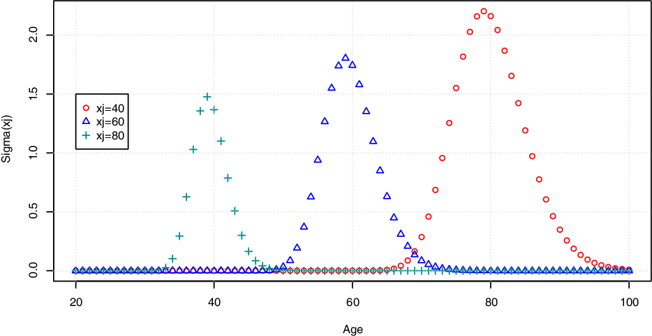
where $\sigma_{0},\sigma_{1}$ , and $\sigma_{2}\in\mathbb{R}^{+}$ . With such a specification, the variance of mortality rates increases exponentially with age, whereas the covariance between $\mu_{t,x_{j}}$ and $\mu_{t,x_{k}}$ is proportional to a normal kernel valued at $|j-k|$ . For this choice of $\Sigma(x_{j})$ , the covariance of variations of mortality rates for close (resp. distant) ages is high (resp. low). Figure 4 illustrates the structure of correlation between mortality rates, generated with a vector $\Sigma(.)$ such as defined by Equation (4.1). In this framework, mortality rates are locally correlated to their close neighborhood which size is determined by the parameter $\sigma_{2}$ . The covariance function $\Sigma(.)$ is similar to the squared exponential (SE) kernel used by Wu and Wang (Reference Wu and Wang2018) who propose a Gaussian process regression for mortality rates. SE kernels are also commonly used in spatial statistics, and we refer the reader to Adler (Reference Adler1981) for details.

For non-integer ages, $\Sigma(x)$ is set to closest $\Sigma(x_{j})$ -value :

\begin{eqnarray*}\Sigma(x) & = & \left\{ \Sigma(x_{j})\,|\,j=\arg\min_{k\in\{1,...,p\}}|x-x_{k}|\right\} \,.\end{eqnarray*}

Figure 4.

$\Sigma(x_{j})$ for $x_{j}=40,60,80$ with $\sigma_{0}=1$ , $\sigma_{1}=0.01$ , and $\sigma_{2}=0.09$ .

In numerical illustrations, we assume that the baseline mortality is a Gompertz–Makeham function. Nevertheless, we draw the attention of the reader that the estimation procedure is not constrained by the choice of the volatility and baseline mortality functions. Any other specification may be considered under the condition that $d=p$ . The next proposition is a key result to filter the longevity process.

Proposition 4.1. Let us denote the vector of mortality rates by $\boldsymbol{\mu}_{t}=\left(\mu_{t,x}\right)_{x=x_{1},...,x_{p}}$ . In the absence of shock on the longevity process ( $L_{t}=0$ , for all $t\geq0$ ), $\left(\boldsymbol{\mu}_{t+1},\theta_{t+1}\,|\,\boldsymbol{\mu}_{t},\theta_{t}\right)$ is a multivariate normal distribution:

(4.2) \begin{eqnarray}\left(\left.\left(\begin{array}{c}\theta_{t+1}\\[5pt] \boldsymbol{\mu}_{t+1}\end{array}\right)\right|\left(\begin{array}{c}\theta_{t}\\[5pt] \boldsymbol{\mu}_{t}\end{array}\right)\right) & \sim & N\left(\left(\begin{array}{c}m_{\theta}(t,\boldsymbol{\mu}_{t},\theta_{t})\\[5pt] m_{\boldsymbol{\mu}}(t,\boldsymbol{\mu}_{t},\theta_{t})\end{array}\right),\left(\begin{array}{cc}\sigma_{\theta}^{2} & \sigma_{\boldsymbol{\mu},\theta}^{\top}\\[5pt] \sigma_{\boldsymbol{\mu},\theta} & \sigma_{\boldsymbol{\mu}}^{2}\end{array}\right)\right)\,,\end{eqnarray}

where $m_{\theta}(t,\boldsymbol{\mu}_{t},\theta_{t})$ and $m_{\boldsymbol{\mu}}(t,\boldsymbol{\mu}_{t},\theta_{t})=\left(m_{\boldsymbol{\mu}}(t,\mu_{t,x_{j}},\theta_{t})\right)_{j=1,...,p}$ are respectively a scalar and a p-vector equal to

(4.3) \begin{eqnarray} & & m_{\theta}(t,\boldsymbol{\mu}_{t},\theta_{t})=e^{-\alpha}\theta_{t}+\bar{\theta}\!\left(1-e^{-\alpha}\right)+\frac{\alpha(\theta_{0}-\bar{\theta})}{\alpha-\gamma}e^{-\gamma t}\left(e^{-\gamma}-e^{-\alpha}\right), \end{eqnarray}

(4.4) \begin{eqnarray} m_{\boldsymbol{\mu}}(t,\mu_{t,x_{j}},\theta_{t})&=&e^{-\kappa}\mu_{t,x_{j}}+\frac{\kappa\theta_{t}\mu(x_{j})\left(e^{-\alpha}-e^{-\kappa}\right)}{\kappa-\alpha}\\[5pt] & & +\,\mu(x_{j})\frac{\kappa\alpha\bar{\theta}}{\kappa-\alpha}\left(\frac{1}{\alpha}\left(1-e^{-\alpha}\right)-\frac{1}{\kappa}\left(1-e^{-\kappa}\right)\right)\nonumber \\[5pt] & & +\,\mu(x_{j})\frac{\kappa\alpha\!\left(\theta_{0}-\bar{\theta}\right)e^{-\gamma t}}{\kappa-\alpha}\left(\frac{e^{-\gamma}-e^{-\alpha}}{\alpha-\gamma}-\frac{e^{-\gamma}-e^{-\kappa}}{\kappa-\gamma}\right)\,.\nonumber\end{eqnarray}

The variance of $\theta_{t+1}\,|\,\boldsymbol{\mu}_{t},\theta_{t}$ is equal to $\sigma_{\theta}^{2}=\frac{\nu^{2}}{2\alpha}\left(1-e^{-2\alpha}\right)$ . The covariance vector $\sigma_{\boldsymbol{\mu},\theta}=\left(\sigma_{\boldsymbol{\mu},\theta}(x_{j})\right)_{j=1,...,p}$ of dimension $p-1$ is given by 4.

(4.5) \begin{eqnarray}\sigma_{\boldsymbol{\mu},\theta}(x_{j}) & = & \nu^{2}\frac{\kappa\mu(x_{j})}{\kappa-\alpha}\left(\frac{1}{2\alpha}\left(1-e^{-2\alpha}\right)-\frac{1}{\alpha+\kappa}\left(1-e^{-\left(\alpha+\kappa\right)}\right)\right)\,.\end{eqnarray}

The ( $p-1)\times(p-1)$ covariance matrix $\sigma_{\boldsymbol{\mu}}^{2}=\left(\sigma_{\boldsymbol{\mu}}^{2}(x_{j},x_{k})\right)_{j,k=1,...,p}$ contains the following elements:

(4.6) \begin{align} \sigma_{\mu}^{2}(x_{j},x_{k})&=\frac{\Sigma(x_{j})^{\top}\Sigma(x_{k})}{2\kappa}\left(1-e^{-2\kappa}\right)+\mu(x_{j})\mu(x_{k})\left(\frac{\kappa\nu}{\kappa-\alpha}\right)^{2}\\[5pt] & \quad\times\left(\frac{1}{2\alpha}\left(1-e^{-2\alpha}\right)+\frac{1}{2\kappa}\left(1-e^{-2\kappa}\right)-\frac{2}{\alpha+\kappa}\left(1-e^{-\left(\alpha+\kappa\right)}\right)\right)\,.\nonumber\end{align}

If $\boldsymbol{\mu}_{t+1}$ and $\theta_{t+1}$ would be both observable, we could estimate the model by maximizing the log-likelihood of the distribution (4.2). In practice, $\theta_{t+1}$ is not directly visible and we need to filter it. We exploit the properties of the multivariate normal distribution to find an estimate, noted $\widehat{\theta}_{t+1}$ of $\theta_{t+1}$ . In the absence of jump, we know that that the conditional expectation of $\theta_{t+1}$ is related to parameters of the multivariate normal (4.2) as follows:

\begin{eqnarray*}\mathbb{E}\!\left(\theta_{t+1}|\boldsymbol{\mu}_{t+1},\boldsymbol{\mu}_{t},\theta_{t}\right) & = & m_{\theta}(t,\boldsymbol{\mu}_{t},\theta_{t})+\sigma_{\boldsymbol{\mu},\theta}^{\top}\left(\sigma_{\boldsymbol{\mu}}^{2}\right)^{-1}\left(\boldsymbol{\mu}_{t+1}-m_{\boldsymbol{\mu}}(t,\boldsymbol{\mu}_{t},\theta_{t})\right),\end{eqnarray*}

and its conditional variance is equal to

\begin{eqnarray*}\mathbb{V}\!\left(\theta_{t+1}|\boldsymbol{\mu}_{t+1}\right) & = & \sigma_{\theta}^{2}-\sigma_{\boldsymbol{\mu},\theta}^{\top}\left(\sigma_{\boldsymbol{\mu}}^{2}\right)^{-1}\sigma_{\boldsymbol{\mu},\theta}\,.\end{eqnarray*}

Therefore, a natural recursive estimator of $\theta_{t+1}$ , based on the observation of mortality rates and previous filtered values of the longevity process is provided by:

(4.7) \begin{eqnarray}\widehat{\theta}_{t+1} & = & \mathbb{E}\!\left(\theta_{t+1}|\boldsymbol{\mu}_{t+1},\boldsymbol{\mu}_{t},\widehat{\theta}_{t}\right)\\[5pt] & = & m_{\theta}(t,\boldsymbol{\mu}_{t},\widehat{\theta}_{t})+\sigma_{\boldsymbol{\mu},\theta}^{\top}\left(\sigma_{\boldsymbol{\mu}}^{2}\right)^{-1}\left(\boldsymbol{\mu}_{t+1}-m_{\boldsymbol{\mu}}(t,\boldsymbol{\mu}_{t},\widehat{\theta}_{t})\right)\,.\nonumber\end{eqnarray}

For a given set of parameters, we filter recursively $\left(\theta_{t}\right)_{t\geq0}$ with Equation (4.7). The matrix $\sigma_{\boldsymbol{\mu}}^{2}$ is inverted by singular value decomposition (SVD). We first compute the $d\times d$ matrix U, $\Lambda$ , and V where $\Lambda$ is diagonal and such that $\sigma_{\boldsymbol{\mu}}^{2}=U\Lambda V^{\top}$ . The inverse is $\left(\sigma_{\boldsymbol{\mu}}^{2}\right)^{-1}=U\Lambda^{-1}V^{\top}$ . After the filtration of $\widehat{\theta}_{t}$ , the log-likelihood of the sample of observations, denoted by $\ln L$ , is approached by the following sum:

(4.8) \begin{eqnarray}\ln L & = & \sum_{t=0}^{n-1}\ln\!\left(f_{\boldsymbol{\mu}}\left(\boldsymbol{\mu}_{t+1}|m_{\boldsymbol{\mu}}(t,\boldsymbol{\mu}_{t},\widehat{\theta}_{t})\,,\,\sigma_{\boldsymbol{\mu}}^{2}\right)\right)\end{eqnarray}

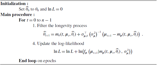
where $f_{\boldsymbol{\mu}}\left(\,.\,|\,m_{\boldsymbol{\mu}},\sigma_{\boldsymbol{\mu}}^{2}\right)$ is the probability density function of a multivariate normal with mean $m_{\boldsymbol{\mu}}$ and covariance matrix $\sigma_{\boldsymbol{\mu}}^{2}$ . Algorithm 1 summarizes the procedure to compute the log-likelihood. For a model without jump, the parameter estimates are next found by maximizing the log-likelihood (4.8) in which $\left(\theta_{t}\right)_{t\geq0}$ is replaced by its filtered values $\left(\widehat{\theta}_{t}\right)_{t\geq0}$ .

Algorithm 1

Procedure to compute the log-likelihood of a sample of observations, model with no jump.

Proposition 4.1 and Algorithm 1 allow us to fit a model without jump. The estimation by log-likelihood maximization of the model with jump risk is a challenging task because the multivariate distribution of $\left(\boldsymbol{\mu}_{t},\theta_{t}\right)$ and the conditional distribution $\theta_{t+1}|\boldsymbol{\mu}_{t+1},\boldsymbol{\mu}_{t},\theta_{t}$ are unknown in this case. To remedy this issue, we employ a peak-over-threshold approach, similar to Hainaut (Reference Hainaut2022, Chapter 4, Section 3). This approach is robust and easy to implement. The first stage consists in fitting a Gaussian model without jumps by log-likelihood maximization and in filtering $\{\widehat{\theta}_{0},\widehat{\theta}_{1},...,\widehat{\theta}_{n}\}$ . We next consider the discrete record of n variations $\{\Delta\widehat{\theta}_{1},...,\Delta\widehat{\theta}_{n}\}$ where $\Delta\widehat{\theta}_{k}=\widehat{\theta}_{k}-\widehat{\theta}_{k-1}$ for $k=1,...,n$ . A mortality jump is believed to occur when one of these variations is above a threshold noted $g(\alpha)$ . In practice, $g(\alpha)$ is the $\alpha$ -percentile of the empirical distribution of $\left(\Delta\widehat{\theta}_{k}\right)_{k=1,...,n}$ . The time of the $k{\rm th}$ jump is therefore:

\begin{eqnarray*}t_{k} & = & \min\{t_{j}\in\{1,...,n\}\,|\,\Delta\widehat{\theta}_{j}\geq g(\alpha)\,,\,j\geq k\}\,.\end{eqnarray*}

and the sample path of $\left(N_{t}\right)_{t\geq0}$ is approached by the following time series:

\begin{align*}N(t_{j})=\max\{k\in\mathbb{N}\,|\,t_{k}\leq t_{j}\}\,.\end{align*}

The level of confidence $\alpha$ is chosen such that years during which a jump is detected, correspond to a year during which an abnormal over-mortality is identified (e.g., such as in 2020 due to the COVID 19 pandemics). In numerical illustrations, we set $\alpha$ to 94%. The jump size parameter, $\rho$ , is estimated by log-likelihood maximization under the assumption that the entire variation $\Delta\widehat{\theta}_{k}$ is caused by the jump. This choice is motivated by the difficulty to decompose the yearly variation into Brownian and jump components.

5. Estimation and validation on the Belgian population

We fit the model to the Belgian female and male populations. The data setFootnote 1 contains mortality rates from 1950 to 2010 for the range of ages 20–10 years. The number of Brownian motion is then equal to $d=p=81$ . The baseline mortality, $\mu(x)$ , is the Gompertz–Makeham function. Notice that we can choose any other baseline function without affecting the performance of the estimation procedure. 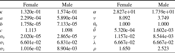Indeed, the Algorithm 1 depends solely on $\mu(x)$ and not of its integral. Parameter estimates found by log-likelihood maximization are reported in Table 1. To avoid identification issues, the parameter $\theta_{0}$ is set to 1. The instantaneous volatility $\nu$ of $\theta_{t}$ is high, but the speed of mean reversion, $\alpha$ , is also high and drives quickly back $\theta_{t}$ to $\beta(t)$ . The mean reversion level $\beta(t)$ of $\theta(t)$ slowly decays from $\theta_{0}$ to a lower value, $\bar{\theta}$ .

Table 1.

Parameter estimates for the 20–100 years old female and male populations, 1950–2010.

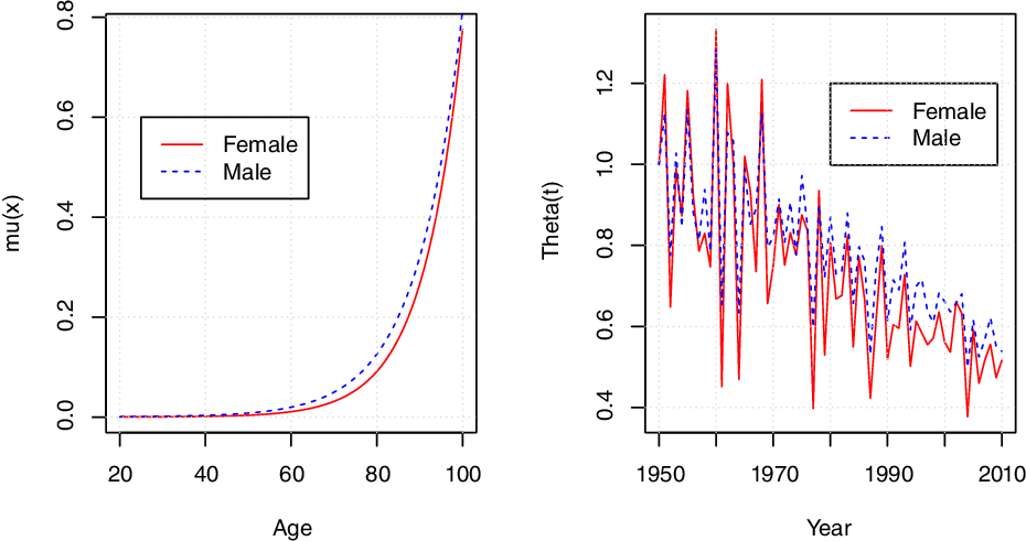
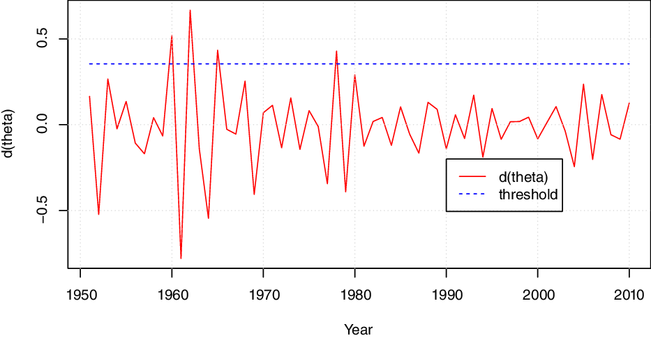
Figures 5 presents calibration results. The left plots shows the estimated baseline mortality functions, $\mu(x)$ . Male baseline rates are slightly higher than female ones. The right plots present filtered values of longevity process, $\widehat{\theta}_{t}$ for $t\in\{1950,...,2010\}$ . Female and male longevity processes decline on average over time, but the decrease is slightly more pronounced for women than for men. This is explained by the fact that the female life expectancy has risen quicker than the one of the male population. 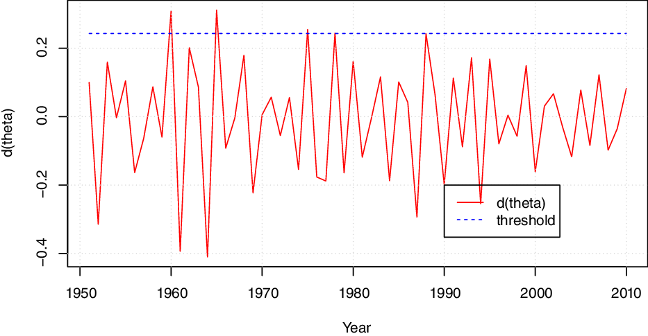Figures 6 and 7 show the variation of female and male longevity processes, $\Delta\widehat{\theta}_{k}$ and the percentile above which a jump is supposed to occur. For the female and male populations and a confidence level of $\alpha=$ 94%, we identify four shocks.

Figure 5.

Belgian female and male populations, 1950–2010, 20 to 100 years old. Left plot: estimated $\mu(x)$ function. Right plot: filtered $\left(\widehat{\theta}_{t}\right)_{t\geq0}$ .

Figure 6.

Belgian female population, jumps detection by peaks over threshold. The red line is $\Delta\widehat{\theta}_{t}=\widehat{\theta}_{t+1}-\widehat{\theta}_{t}$ , and the threshold is the 95% percentile of $\Delta\widehat{\theta}_{t}$ .

Figure 7.

Belgian male population, jumps detection by peaks over threshold. The red line is $\Delta\widehat{\theta}_{t}=\widehat{\theta}_{t+1}-\widehat{\theta}_{t}$ , and the threshold is the 95% percentile of $\Delta\widehat{\theta}_{t}$ .

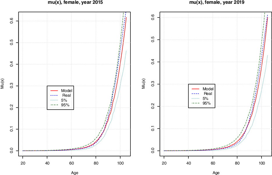
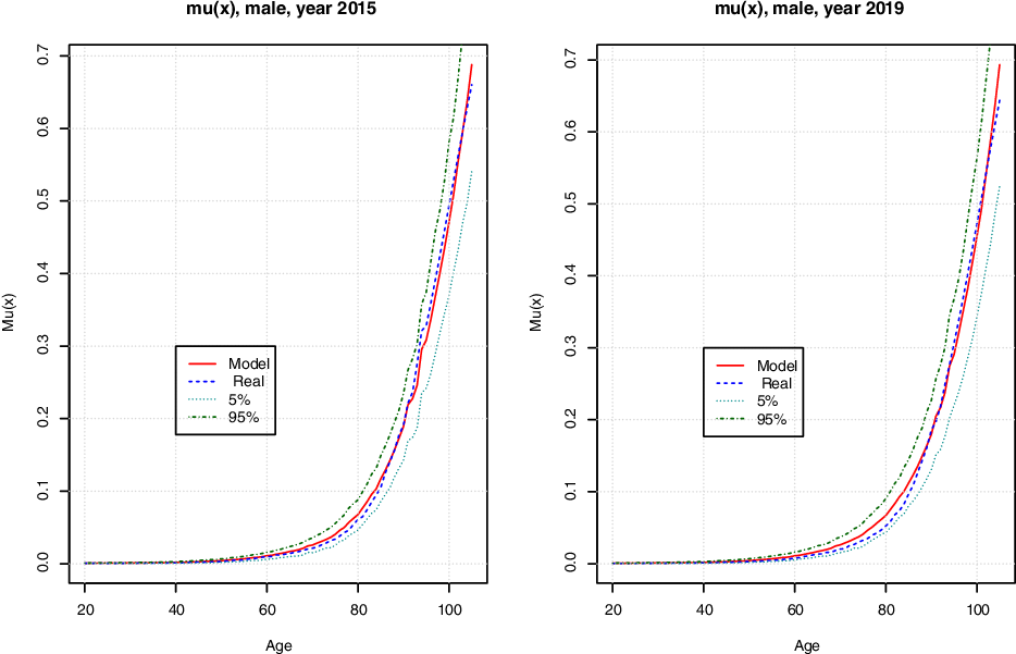
In order to evaluate the predictive power of our model, we generate 1000 mortality scenarios over the period 2011 up to 2020 for ages from 0 up to 105 years. Processes $\mu_{t,x}$ and $\theta_{t}$ are simulated by discretizing Equations (2.2) and (2.3) with a time step equal to $1/300$ . Figures 8 and 9 display statistics about male and female mortality forecasts in 2015 and 2019. For men, the gap between average simulated and observed mortality rates is small. This gap is slightly wider for women, but observed rates are located in the 5–95% confidence interval of simulated rates. This confirms the ability of our model to generate realistic mortality scenarios. We also notice that 5% and 95% percentiles of mortality rates are positive. This observation justifies the Gaussian assumption for the dynamics of $\mu_{t,x}$ and $\theta_{t}$ .

Figure 8.

Female population, forecast mortality rates with parameter estimates fitted to the sample 1950–2010, ages from to 20 to 105.

Figure 9.

Male population, forecast mortality rates with parameter estimates fitted to the sample 1950–2010, ages from to 20 to 105.

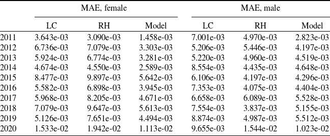
We benchmark our framework to the LC and the Renshaw–Haberman (RH) models, under the assumption that the number of deaths follows a Poisson distribution. For this purpose, we use the R package STMoMo to fit the two first models to Belgian mortality rates from 1950 to 2010 and ages between 20 and 105 years. Let us recall that in the LC and RH models, the mortality rates are ruled by the following equations:

\begin{align*}\ln\mu_{x}(t) & =\alpha_{x}+\beta_{x}\kappa_{t}\\[5pt] \ln\mu_{x}(t) & =\alpha_{x}+\rho_{t-x}+\beta_{x}^{1}\kappa_{t}\end{align*}

where $\kappa_{t}$ explains the global evolution of mortality and $\rho_{t-x}$ represents the cohort effect. Both models are estimated with a Poisson law for the number of deaths. Next, we forecast 1000 mortality scenarios over the period 2011–2020 with standard auto-regressive models AR(1) for $\kappa_{t}$ and $\rho_{t-x}$ . Table 2 reports the mean absolute errors (MAE) between observed and average simulated mortality rates. According to this criterion, our model outperforms the LC and RH approaches from 2011 up to 2019 for the female population. Knowing that the year 2020 is particular due to the over-mortality caused by the COVID-19, this is a remarkable performance. For men, our model outperforms the LC framework up to 2019 and has smaller or similar MAE to the RH model. It is worth to mention that such a good performance of the calendar year model is obtained with only 14 parameters, whereas the LC and RH models count more than 100 coefficients to estimate.

Table 2.

Mean Absolute Errors (MAE) between average simulated and observed mortality rates from 2011 to 2020 and for ages from 20 to 105 years.

Finally, we compare our model to a Gaussian cohort framework in which the mortality rate at time t, of a $x+t$ years old individual is

\begin{align*}\mu_{x+t} & =a_{x}+\lambda_{x+t}\,,\\[5pt] d\lambda_{x+t} & =\kappa_{x}\lambda_{x+t}dt+\sigma_{x}dW_{t}^{x}\,,\end{align*}

where $a_{x}$ , $\kappa_{x}$ , and $\sigma_{x}$ $\in\mathbb{R}^{+}$ . The survival probability in this model, $_{t}p_{x}=\mathbb{E}\!\left(e^{-\int_{0}^{t}\mu_{x+s}ds}\right)$ is equal to

\begin{eqnarray*}_{t}p_{x} & = & \exp\!\left(-\left(a_{x}-\frac{\sigma_{x}^{2}}{2\kappa_{x}^{2}}\right)t-\frac{1}{\kappa_{x}}\left(e^{\kappa_{x}t}-1\right)\left(\lambda_{x}+\frac{\sigma_{x}^{2}}{\kappa_{x}^{2}}-\frac{\sigma_{x}^{2}}{4\kappa_{x}^{2}}\left(e^{\kappa_{x}t}+1\right)\right)\right)\,.\end{eqnarray*}

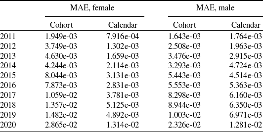
We fit this model to cohorts of ages 30–90 years in 2010. We use the same window of time as for the LC, RH, and calendar year model: Belgian mortality rates from 1950 to 2010. The 60 sets of parameters $\left(a_{x},\kappa_{x},\sigma_{x},\lambda_{x}\right)$ are estimated by least square minimization between observed and modeled survival of probabilities. The model for the youngest cohort is estimated with 20 observations, but we wanted to use data prior to the second world war as sanitary conditions were significantly different from those of the post-war period. We have also sufficient to have a good fit and forecasts at short term. We next use the 60 models to compute mortality rates over the period 2011 (ages 31–91 years) to 2020 (ages 40–100 years). The corresponding MAE’s are reported and compared to these obtained with the calendar year model in Table 3. For the female population, the calendar year model leads to a lower MAE from 2011 to 2020. For the male population, cohort and calendar model have a similar predictive power from 2011 to 2013. At longer term, the MAE computed with the calendar year are the longer. Globally, the calendar year model outperforms the cohort approach. It is also more parsimonious when we need to forecast the mortality of multiple cohorts (in our illustration, 14 instead of 60 $\times$ 4 parameters).

Table 3.

Mean Absolute Errors (MAE) between average simulated and observed mortality rates from 2011 to 2020 and for 30 to 90 years old cohorts in 2010.

6. Estimation over 1950–2020 and life expectancy

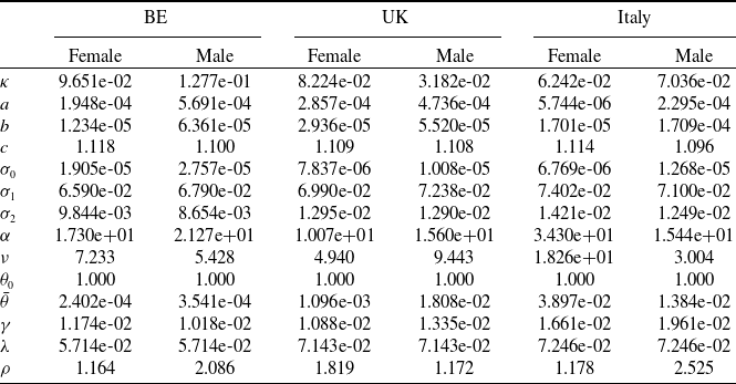
Table 4 presents parameter estimates for Belgium, UK, and Italy. The model is fitted to mortality rates of female and male populations from 1950 up to 2020 (2019 for Italy because the 2020 data is not available yet on HMD) and for ages between 20 and 105 years. As previously, the longevity process is filtered using a subsample of $q=15$ equispaced mortality rates. We observe many similarities between parameters for UK and Belgium. Some parameters for Italy move away from their Belgian and UK equivalents, but this is explained by the longer life expectancy in this country.

Table 4.

Parameter estimates for Belgium, UK, and Italy.

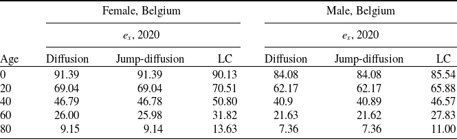
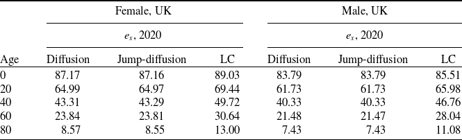
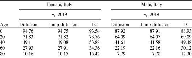
Tables 5, 6, and 7 report the prospective life expectancy in 2020 (2019 for Italy) at 0, 20, 40, 60, and 80 years old. The columns “Diffusion” and “Jump-Diffusion,” respectively, report expectancies computed within a pure Brownian framework and with the jump-diffusion model. Whatever the considered population, these life expectancies are very close (less than 1/10 of year). This emphasizes the small impact of punctual mortality shocks on the evolution of life expectancy. For the year 2019 in Belgium, the (cross-sectional) female and male life expectancies were, respectively, equal to 84.0 years and 79.6 years. In comparison, the prospective life expectancies at birth calculated increase of 7.39 years for women and of 4.48 years for men. The life expectancy at birth in the UK in 2018 to 2020 was 79.0 years for males and 82.9 years for females. Our model forecast a higher prospective life expectancy of 4.79 years for men and of 4.27 years for women. In Italy, the male and female life expectancies were equal to 81.40 and 85.70 years in 2019. In comparison, female and male prospective life expectancies, respectively, rise by 9.06 and by 6.52 years.

Table 5.

Prospective life expectancies, $e_{x}$ , in 2020 at 0, 20, 40, 60, and 80 years old.

Table 6.

Prospective life expectancies, $e_{x}$ , in 2020 at 0, 20, 40, 60, and 80 years old.

Table 7.

Prospective life expectancies, $e_{x}$ , in 2019 at 0, 20, 40, 60, and 80 years old.

Tables 5, 6, and 7 also report the prospective life expectancies computed with the LC model (column LC). The expectation at birth predicted by calendar year and LC models are relatively close to each other. A gap appears for life expectancies at older ages. We explain this gap by the trend of the model to overestimate mortality rates between 60 and 85 years of age. This overestimation is clearly visible in Figures 8 and 9 and is partly due to shape of the Makeham–Gompertz law.

7. Pricing and risk management

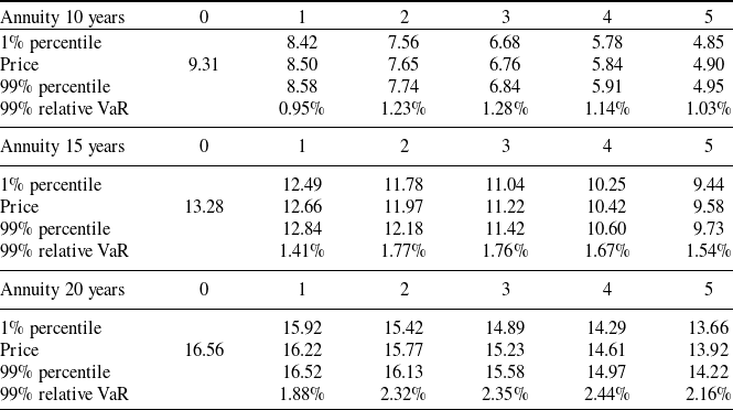
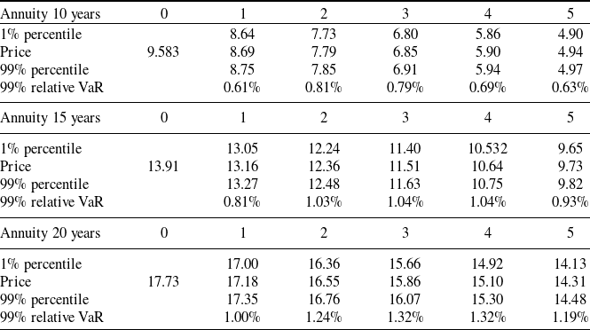
In this last section, we test the capacity of our model to evaluate a term life annuity and the related longevity risk. We consider annuities with three maturities 10, 15, and 20 years. They are valued with parameter estimates of Table 4 for a 60-year-old Belgian woman and man. The valuation is then done under the real measure P. The interest rate r is set to 0%. Prices are reported in the columns “0” of Tables 8 and 9. The female longevity being higher that the male one, annuity prices are slightly more expensive for women than for men.

Table 8.

Annuity values and percentiles over the first 5 years, male, Belgium.

Table 9.

Annuity values and percentiles over the first 5 years, female, Belgium.

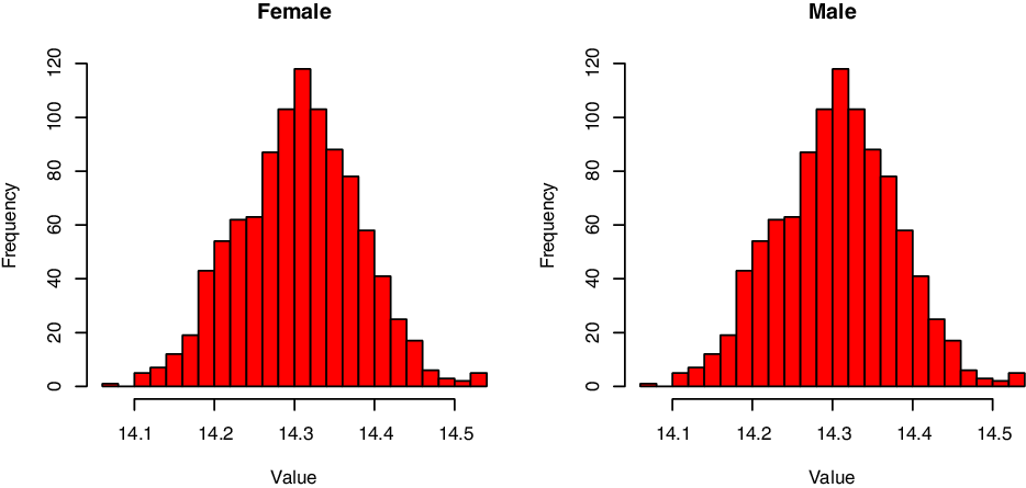
As emphasized in Section 3, we do not need to perform simulations in simulations for determining the distribution of future values as survival probabilities admit a closed-form expression. To illustrate this, we simulate a sample of 1000 mortality rates over a period of 5 years. Annuities are re-evaluated in each scenario at the end of each year. Figure 10 shows the histogram of 20 years annuity values after 5 years. Both for male and female, we observe a small left asymmetry.

Figure 10.

Simulated values in 5 years of an annuity with an initial maturity of 20 years. 1000 simulations.

The average values, the 1% and 99% percentile of annuity values, are reported in columns “1” up to “5” of Tables 8 and 9. The exposure to the longevity risk is measured by the 99% relative Value at Risk (VaR), computed as the spread between average and percentile values divided by the average price. This exposure is higher for men than for women, whatever the duration of the annuity. This is explainable by the difference between male and female life expectancies. Women live on average longer than men and therefore cash flows paid by a term life annuity are less volatile. This drives up prices of female annuity and decreases the uncertainty related to premature deaths. The VaR for male and female, respectively, climbs up to 2.44% and 1.32% for a 20-year annuity.

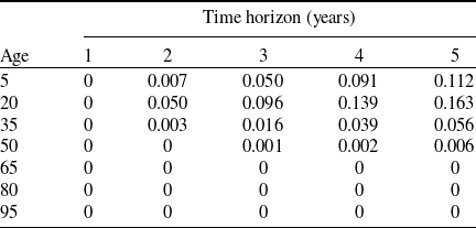
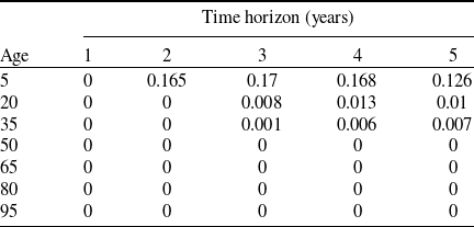
To conclude this section, we analyze the probability of generating negative mortality rates. Tables 10 and 11 report the probability of generating negative mortality rates by ages and time horizons, for the Belgian female and male populations. We observe that this probability is the higher for younger ages (ages at which the average mortality is quasi null) but becomes null or neglible after 35 years old. This confirms the reliability of our model for modeling longevity for the usual annuitants range of ages.

Table 10.

Probability of generating negative mortality rates by ages and time horizons. Belgian female population.

Table 11.

Probability of generating negative mortality rates by ages and time horizons. Belgian male population.