





1. Introduction
Active flow control (AFC) has emerged as a relevant strategy to enhance the aerodynamic performance of ground and air vehicles (Brunton & Noack Reference Brunton and Noack2015). By manipulating flow separation and wake structures using actuators such as synthetic jets, plasma devices or moving surfaces, significant performance gains can be achieved (Greenblatt & Wygnanski Reference Greenblatt and Wygnanski2000; Glezer & Amitay Reference Glezer and Amitay2002; Cattafesta & Sheplak Reference Cattafesta and Sheplak2011). For ground vehicles, the efficacy of open-loop actuation has been well demonstrated in wind tunnel studies on simplified bluff bodies, where steady and pulsed blowing can substantially recover base pressure and reduce drag (Littlewood & Passmore Reference Littlewood and Passmore2012; McNally et al. Reference McNally, Fernandez, Robertson, Kumar, Taira, Alvi, Yamaguchi and Murayama2015; Cerutti et al. Reference Cerutti, Sardu, Cafiero and Iuso2020; Amico et al. Reference Amico, Cafiero and Iuso2022, Reference Amico, Serpieri, Iuso and Cafiero2024; Robledo et al. Reference Robledo, Alfaro, Duro, Solera-Rico, Castellanos and Sanmiguel Vila2026).
Feedback control promises further significant improvements (Brunton & Noack Reference Brunton and Noack2015). Real-world conditions are inherently unsteady, and an effective AFC system must be able to sense the current flow state, predict its evolution and apply an optimal control action that is adapted in real time. To meet these demands, data-driven methods and machine learning are now opening new research avenues (Brunton et al. Reference Brunton, Noack and Koumoutsakos2020). Broadly, these approaches fall into two categories: model-free controllers that learn a policy directly from data, and model-based controllers that exploit an explicit dynamical model.
Model-free strategies can be attractive when little is known a priori about the system. Such approaches have shown promising results in low-Reynolds-number or numerically simulated flows where large amount of training data are generated in a cheap and safe manner (Garcia et al. Reference Garcia, Miró, Suárez, Alcántara-Ávila, Rabault, Font, Lehmkuhl and Vinuesa2025; Suárez et al. Reference Suárez, Alcántara-Ávila, Rabault, Miró, Font, Lehmkuhl and Vinuesa2025). However, model-free methods are often sample inefficient, provide less transparent guarantees on stability and safety and struggle to incorporate hard constraints on actuators or states. These limitations are particularly restrictive in experimental AFC, where data are expensive and hardware must operate within strict bounds. This motivates a focus on model-based approaches, where control decisions are derived from an explicit predictive model.
A typical example of model-based control is model predictive control (MPC) (Camacho & Bordons Reference Camacho and Bordons2013; Rawlings et al. Reference Rawlings, Mayne and Diehl2017). At each time step, MPC leverages a model of the dynamics to forecast future flow states over a finite horizon and solves an optimisation problem to obtain the optimal control sequence. Compared with purely model-free strategies, this framework is more sample efficient, offers clearer routes to stability and safety guarantees and handles constraints naturally. The primary challenge is therefore the development of a predictive model that is both sufficiently accurate to capture the controlled dynamics and computationally efficient for real-time execution (Kaiser et al. Reference Kaiser, Kutz and Brunton2018; Bieker et al. Reference Bieker, Peitz, Brunton, Kutz and Dellnitz2020; Marra et al. Reference Marra, Meilán-Vila and Discetti2024b ; Liu et al. Reference Liu, Beckers and Eldredge2025; Solera-Rico et al. Reference Solera-Rico, Sanmiguel Vila and Discetti2026).
The effectiveness of MPC ultimately hinges on the reliability of the plant model. In turbulent flows, the difficulty is not only to approximate the unforced dynamics, but also to represent how actuation reshapes the accessible state space. Recent studies show that controlled wakes often evolve on low-dimensional, actuation-dependent manifolds (Marra et al. Reference Marra, Cornejo Maceda, Meilán-Vila, Guerrero, Rashwan, Noack, Discetti and Ianiro2024a ). Reduced coordinates learned without accounting for control inputs may thus yield a latent dynamics that is unnecessarily complex or even inconsistent with feasible actuation commands. This perspective motivates the need to develop actuation-aware reduced-order predictors that remain simple enough for receding-horizon optimisation while capturing the key controlled dynamics.
For this reason, this work focuses on the central challenge of building predictive models suitable for model-based control. While being a gold standard and highly informative in predictive-control implementations (Bewley et al. Reference Bewley, Moin and Temam2001), full-order simulations are computationally intractable in real-time loops. We thus focus on a framework based on reduced-order models (ROMs), with two stages: (i) compress the high-dimensional velocity field into a low-dimensional latent space (the encoding stage), and (ii) learn a time-stepping model that predicts the latent evolution under actuation (the prediction step). This approach has been recently explored by several studies with data-driven methods (Maulik et al. Reference Maulik, Lusch and Balaprakash2021; Bukka et al. Reference Bukka, Gupta, Magee and Jaiman2021; Solera-Rico et al. Reference Solera-Rico, Sanmiguel Vila, Gómez-López, Wang, Almashjary, Dawson and Vinuesa2024). This separation is consistent with many classical ROM pipelines, where the compression step is based on proper orthogonal decomposition (POD): since POD is a purely energy-based decomposition, the resulting latent basis is not explicitly optimised jointly with the subsequent dynamical estimator. While the merits of such techniques are already apparent, we identify two research gaps. On the one hand, the generalisation capabilities of these methods under different exogenous inputs are not clear, and a recipe for training and predicting under environments with active control has not been consolidated yet. On the other hand, there is a growing tendency towards using powerful encoders, while it is not clear if an Occam’s razor solution could be more effective under some configurations. Wake flows, for instance, often evolve on low-dimensional attractors, with a rather predictable dynamics. In flows dominated by vortex shedding, the leading POD coefficients often exhibit a narrow-band, nearly oscillatory dynamics because POD isolates the most energetic coherent structures. In special cases, such as nearly periodic flows, these structures may align with Koopman-related spectral components (Rowley et al. Reference Rowley, Mezić, Bagheri, Schlatter and Henningson2009; Mezić Reference Mezić2013; Taira et al. Reference Taira, Brunton, Dawson, Rowley, Colonius, McKeon, Schmidt, Gordeyev, Theofilis and Ukeiley2017). However, it must be remarked that, even though POD is a linear decomposition, it does not imply that a linearised dynamics is achievable in its reduced space. Therefore, any analogy between the dynamics of the leading POD coefficients and Koopman modes should be understood as problem-dependent rather than intrinsic to POD. On the other hand, convolutional autoencoders (CAEs) can be driven to approximate Koopman operators (Lusch et al. Reference Lusch, Kutz and Brunton2018), although, generally speaking, training driven by reconstruction compactness does not entail robustness guarantees on the dynamics. Existing comparisons between POD and CAE have been targeted already for systems with autonomous dynamics (Fresca et al. Reference Fresca, Dede’ and Manzoni2021; Fresca & Manzoni Reference Fresca and Manzoni2022); however, the interaction between the encoder choice and multi-input actuation, on actuation-dependent manifolds, remains less explored.
To address the gaps above, we compare linear and nonlinear options for encoding, considering wake flow systems under control actions. For encoding, we contrast the classical energy-optimal POD (Sirovich Reference Sirovich1987) with nonlinear CAEs (Solera-Rico et al. Reference Solera-Rico, Sanmiguel Vila, Gómez-López, Wang, Almashjary, Dawson and Vinuesa2024), which typically yield more compact latent representations but may induce a more complex controlled latent dynamics. For temporal prediction, we employ long short-term memory (LSTM) networks (Hochreiter & Schmidhuber Reference Hochreiter and Schmidhuber1997), which are well suited for sequential latent dynamics. Using two two-dimensional (2-D) wake flows, a simplified truck model (Solera-Rico et al. Reference Solera-Rico, Sanmiguel Vila and Discetti2026) and the fluidic pinball (Deng et al. Reference Deng, Noack, Morzyński and Pastur2020), we quantify the trade-off between compactness and forecast accuracy of the latent-space dynamics, and show how the preferred reduction strategy depends on the prediction horizon required by the controller.
The paper is organised as follows. Section 2 provides a description of the methodology, including the generation of data for the chosen test cases. The analysis of the model results is provided in § 3. Finally, the conclusions are discussed in § 4.
2. Methodology
This section details the methodology to develop and evaluate predictive ROMs. First, we describe the two flow configurations and the generation of their respective high-fidelity direct numerical simulation (DNS) datasets. Next, we present the two methods used to encode the high-dimensional spatial fields into a low-dimensional latent space. Finally, in § 2.3, we detail three approaches based on LSTM network architectures for predicting the temporal evolution of this latent space in response to control inputs. The proposed ROM framework is illustrated schematically in figure 1.
2.1. Flow configurations and data generation
Two different 2-D wake flow configurations are used to assess the control architectures. These cases are chosen to represent different control challenges: the first is a single-input system, while the second is a more complex multi-input problem. Both datasets are created using DNSs with open-loop control signals designed to excite the underlying flow dynamics. In low-Reynolds-number flows, DNS provides a simulation framework with minimal numerical approximations to precisely represent the flow dynamics and capture all scale features. The following sections describe the set-up for each case in detail, and a summary of the datasets can be found in table 1.
Summary of the datasets for the two flow configurations.

Table 1. Long description
The table has three columns: Parameter, Simplified truck and Fluidic pinball, and eight parameter rows. Reynolds number is 500 for the truck and 150 for the pinball. Control type is single-input synthetic jets for the truck and multi-input rotating cylinders for the pinball. The control signal is filtered random for the truck and quasi-stationary step ramps for the pinball, with control dimension 1 and 3 respectively. Total snapshots are 50,000 for the truck and 70,000 for the pinball, of which 5,000 and 20,000 are test snapshots. The time step is 0.2 convective times for the truck and 0.1 convective times for the pinball, and the spatial resolution is 128 by 256 grid points for the truck and 96 by 192 for the pinball.
Schematic of the data-driven reduced-order modelling framework. High-dimensional input velocity fields are compressed into a low-dimensional latent-space time series using an encoder (POD or CAE). This latent state, along with the corresponding control sequence, is fed into a temporal predictor to infer the future evolution of the latent space. Finally, a decoder reconstructs the predicted latent states back into the high-dimensional, full-field velocity state space.

Figure 1. Long description
The diagram reads left to right. On the left, a box labelled input holds a stack of vorticity field snapshots at times t minus L, t minus 1 and t, each showing the three pinball cylinders and their wake. A trapezoidal encoder narrows this stack into a small block labelled latent space, holding a few latent time series. Below it a second block labelled control vector holds the corresponding step-like actuation signals. Both feed a tall block labelled Predictor, whose output is a wider block labelled augmented latent space containing the predicted latent time series. A second trapezoidal block, the decoder, expands this into the box labelled output on the right, a stack of reconstructed vorticity snapshots at times t plus 1, t plus 2 and t plus H.
2.1.1. Simplified 2-D truck model
This first case is a simplified model of a wake flow around a road vehicle. Figure 2 depicts the flow configuration based on the horizontal mid-plane geometry of the ground transportation system (Storms et al. Reference Storms, Ross, Heineck, Walker, Driver, Zilliac and Bencze2001), a standard truck model also studied in recent work (McArthur et al. Reference McArthur, Burton, Thompson and Sheridan2016). The model under study is a rectangular bluff body with a reference non-dimensional width
 $W=1$
, length
 $L = 7.647W$
and rounded leading edges with radius
 $r=0.118W$
. The inflow velocity is uniform with a magnitude of
 $U_\infty$
, and the Reynolds number, defined as
 $\textit {Re} = U_\infty W / \nu$
, where
 $\nu$
represents the fluid kinematic viscosity, is set to
 $500$
. The rectangular computational domain extends across the range
 $(-7W, 23W)$
in the streamwise direction (
 $x$
) and
 $(-7.5W, 7.5W)$
in the transverse direction (
 $y$
), with the front of the bluff body placed at
 $x = 0$
. The simulation domain employs a hybrid mesh, structured near the wall and unstructured elsewhere, encompassing around
 $168\,000$
cells. The time is scaled using the convective time
 $t_c=W/U_\infty$
. The DNS is executed in OpenFOAM, using the Gym-preCICE (Shams & Elsheikh Reference Shams and Elsheikh2023) wrapper for the coupling library (Chourdakis et al. Reference Chourdakis2022) and the OpenFOAM adapter (Chourdakis et al. Reference Chourdakis, Schneider and Uekermann2023) to integrate the simulation with the specified control sequence. This Reynolds number is chosen as a representative bluff-body wake configuration to develop and validate control-oriented ROMs before scaling to higher-
 $\textit {Re}$
turbulent regimes. At
 $\textit {Re} = 500$
the wake already exhibits the features relevant to this study, namely vortex shedding and sensitivity to base actuation, while the 2-D flow assumption remains valid, as verified in advance with a 3-D simulation. The compactness–predictability trade-off identified in this work, rooted in the spectral organisation of POD versus the broadband character of the CAE latent dynamics, is not expected to be specific to this Reynolds-number regime; an explicit assessment at higher
 $\textit {Re}$
and in 3-D configurations is left for future work.
Schematic of the simplified truck flow configuration. Zero-net-mass flow jets are illustrated in blue.

The control is implemented using two opposing flow jets at the sides of the vehicle base with zero-net-mass flow, similar to previous experimental set-ups (Barros et al. Reference Barros, Borée, Noack, Spohn and Ruiz2016; Cerutti et al. Reference Cerutti, Sardu, Cafiero and Iuso2020). In this case, the overall mass flow rate of the two jets combined is forced to be zero at each instant of the simulation. The jets, each with a width of
 $w_{\textit{jet}}=0.05W$
, exhibit parabolic velocity profiles with a maximum mean velocity of
 $1.5U_\infty$
. The dataset comprises a time series of velocity fields, with a time increment of
 $\Delta t = t_c/5 = W/{5U_\infty }$
. Figure 3 illustrates the global mesh and a flow sample around the jet region.
Direct numerical simulation mesh and flow details near the base of the truck when jets operate at peak suction/blowing. The symbol
 $U_x$
in the inset indicates the streamwise velocity component. Figure adapted from Solera-Rico et al. (Reference Solera-Rico, Sanmiguel Vila and Discetti2026).

The control input for the simplified truck configuration was generated using a filtered-noise excitation strategy to ensure a rich broadband excitation. First, a discrete white Gaussian noise sequence was generated
 \begin{equation} \xi _n \sim \mathcal{N}(0,1), \end{equation}
where
 $n \in \mathbb{N}_0$
represents the discrete time step index. This index corresponds to the physical time
 $t_n = n\Delta t$
, with a control update interval of
 $\Delta t = 0.2 t_c$
.
To target the relevant flow dynamics, this stochastic sequence was processed through a fourth-order Butterworth bandpass filter, denoted by the operator
 $\mathcal{B}_4$
 \begin{equation} \tilde {\xi }_n = \mathcal{B}_4 \left ( \xi _n; f_{\mathit{low}}, f_{\mathit{high}} \right )\!. \end{equation}
The filter cutoff frequencies were set to
 $f_{\mathit{low}} = 0.05 t_c^{-1}$
and
 $f_{\mathit{high}} = 0.5 t_c^{-1}$
to encompass the wake’s natural shedding frequency of
 $f_{sh} \approx 0.2 t_c^{-1}$
. The filter was applied in a zero-phase (forward–backward) configuration to prevent distortion.
Finally, the filtered sequence
 $\tilde {\xi }_n$
was bounded to reflect the physical limits of the synthetic jets and scaled to determine the applied jet flow rate,
 $b(t_n)$
 \begin{equation} b(t_n) = \dot {m}_{\mathit{max}} \min \big ( 1, \max \big ( -1, \tilde {\xi }_n \big ) \big ), \end{equation}
where the maximum volumetric flow rate capacity of the actuator is
 $\dot {m}_{\mathit{max}} = 0.075 U_{\infty } W$
. During the simulation, the environment linearly interpolated the commanded values between the discrete points
 $t_n$
and
 $t_{n+1}$
to provide a continuous forcing signal to the DNS solver.
Following the simulation, a data preprocessing pipeline was executed to convert the raw OpenFOAM output into a structured dataset. The velocity fields (with
 $u, v$
being respectively the streamwise and cross-wise velocity components) were first interpolated onto a uniform Cartesian grid of
 $128 \times 256$
points using cubic interpolation. This grid spans the domain from
 $x/W = -6$
to
 $x/W = 22$
and
 $y/W = -7$
to
 $y/W = 7$
. A mask was applied to set to zero the velocity in the grid points inside the truck body. The velocity fields
 $\boldsymbol{U}(\boldsymbol{x}, t)$
were then normalised by subtracting the temporal mean field,
 $\boldsymbol{\bar {U}}(\boldsymbol{x})$
, and dividing the components
 $u$
and
 $v$
by their respective global scalar standard deviations (
 $\sigma _u$
,
 $\sigma _v$
), calculated throughout the entire dataset. In parallel, the actual jet flow rate was extracted from post-processing files and time synchronised with the velocity snapshots. The final
 $10\,\%$
snapshots of the long sequence were used for testing, with the remaining used for training.
2.1.2. Fluidic pinball
The second test case is the fluidic pinball, a canonical 2-D set-up often used for complex multi-input multi-output control problems (Deng et al. Reference Deng, Noack, Morzyński and Pastur2020), schematised in figure 4. The geometry consists of three cylinders of equal diameter
 $D=2R$
, with their centres located at the vertices of an equilateral triangle. The centre-to-centre side length of the triangle is
 $3R$
. The origin of the reference system is located in the midpoint between the two centres of the downstream cylinders, with the
 $x$
axis pointing in the direction and the sense of the free-stream velocity
 $U_\infty$
and the
 $y$
axis perpendicular to it in the transverse direction. The rectangular computational domain extends from
 $(-5D, 15D)$
in the streamwise (
 $x$
) direction and
 $(-5D, 5D)$
in the transverse (
 $y$
) direction.
Schematic of the fluidic pinball flow configuration.

The dataset for this configuration was generated with a solver based on an implicit time integration finite element method. The Reynolds number is set to
 $\textit {Re}=150$
, higher than the transition point
 $\textit {Re} \simeq 115$
from a quasi-periodic asymmetric regime to chaotic flow (Deng et al. Reference Deng, Noack, Morzyński and Pastur2020, Reference Deng, Noack, Cornejo Maceda and Pastur2025). This regime exhibits a dominant vortex shedding with random upward and downward switches in the centre jet, remaining as a challenging dynamical system. The time is scaled using the convective time
 $t_{c}=D/U_\infty$
. The resulting dataset contains the 2-D velocity fields (
 $u, v$
) for each time step, normalised with the free-stream velocity
 $U_\infty$
. Control is applied by changing the tangential speed of the three cylinder surfaces, providing three independent control parameters. Notice that the input speeds are normalised with
 $U_\infty$
and defined positive when the rotation is set to be counter-clockwise.
The control set-up for the fluidic pinball configuration was designed as a multi-input strategy using quasi-stationary step ramps to excite the dynamics of the system. The control inputs are defined by the normalised tangential speeds of the three cylinders,
 $\boldsymbol{b}(t) = [b_1(t), b_2(t), b_3(t)]^{\top}$
, corresponding to the top, bottom and forward cylinders, respectively.
To cover the control spectrum, target speed combinations, denoted as
 $\boldsymbol{v}_k$
, were generated from the
 $125$
possible permutations of discrete rotational speeds
 \begin{equation} \boldsymbol{v}_k \in \mathcal{V}^3, \quad \mathrm{where} \quad \mathcal{V} = \{-1, -0.5, 0, 0.5, 1\}. \end{equation}
For a given target step
 $k$
, each cylinder
 $i \in \{1, 2, 3\}$
maintains its target speed
 $v_{k,i}$
for a constant hold duration of
 $T_{\mathit{hold},i}$
. Following the hold phase, the speed transitions linearly to the subsequent target value
 $v_{k+1,i}$
over a cylinder-specific ramp duration
 $T_{\mathit{ramp},i}$
.
Mathematically, the control signal for cylinder
 $i$
during the transition to the
 $(k+1)$
th step and its subsequent hold phase can be described by the piecewise function
 \begin{equation} b_i(t) = \begin{cases} v_{k,i} + \frac {v_{k+1,i} - v_{k,i}}{T_{\mathit{ramp}, i}} (t - t_{k,i}), & \mathrm{if }\, t_{k,i} \le t \lt t_{k,i} + T_{\mathit{ramp}, i} ,\\[5pt] v_{k+1,i}, & \mathrm{if } \,t_{k,i} + T_{\mathit{ramp}, i} \le t \le t_{k+1,i}, \end{cases} \end{equation}
where
 $t_{k,i}$
marks the beginning of the
 $k$
th ramp for cylinder
 $i$
, and
 $t_{k+1,i} = t_{k,i} + T_{\mathit{ramp}, i} + T_{\mathit{hold}, i}$
is the beginning of the next cycle. The transition durations vary for each actuator, defined as
 $T_{\mathit{ramp}, 1} = 25\,t_c$
for the top cylinder,
 $T_{\mathit{ramp}, 2} = 40\,t_c$
for the bottom cylinder and
 $T_{\mathit{ramp}, 3} = 120\,t_c$
for the forward cylinder. Similarly, the hold durations are also specific to each cylinder, i.e.
 $T_{\mathit{hold}, 1} = 30\,t_c$
,
 $T_{\mathit{hold}, 2} = 235\,t_c$
and
 $T_{\mathit{hold}, 3} = 1250\,t_c$
.
This dataset contains a total of 70 000 snapshots, captured with a time spacing of 0.1 convective times between each snapshot. The final 20 000 snapshots are reserved for testing, with the first 50 000 used for training. Following the simulation, each snapshot of the velocity field was preprocessed and interpolated onto a regular grid, resulting in a final resolution of
 $96 \times 192$
pixels. As with the previous flow configuration, a zero velocity mask is applied to the inner body regions. Both POD and CAE operate on the fluctuating velocity components
 $\boldsymbol{u}(\boldsymbol{x}, t) = \boldsymbol{U}(\boldsymbol{x}, t) - \bar {\boldsymbol{U}}(\boldsymbol{x})$
, normalised by their respective global standard deviations.
2.2. Dimensionality reduction methods
The datasets consist of long time series of full-field velocity field snapshots under different control actions. Attempting to directly predict the temporal evolution of the entire high-dimensional spatial field,
 $\boldsymbol{U}(\boldsymbol{x}, t)$
, is computationally intractable for real-time control applications. The core strategy is therefore to first reduce the high spatial dimensionality of each snapshot into a low-dimensional latent-space representation,
 $\boldsymbol{z}(t) \in \mathbb{R}^d$
, where
 $d \ll N_p$
is the latent dimension, and
 $N_p$
the number of grid points. The subsequent task, detailed in § 2.3, is to build a predictive model that can forecast the temporal evolution of this much smaller state vector. In this work, we implement and systematically compare two canonical families of methods for the spatial dimensionality reduction task: the classical, energy-optimal linear POD, and nonlinear deep CAEs following previous work such as Solera-Rico et al. (Reference Solera-Rico, Sanmiguel Vila, Gómez-López, Wang, Almashjary, Dawson and Vinuesa2024) and Fukagata & Fukami (Reference Fukagata and Fukami2025). Within the nonlinear family, we additionally consider two regularised variational variants, a
 $\beta$
-variational autoencoder (
 $\beta$
-VAE) and a decomposed Kullback–Leibler (KL) variational autoencoder (DKL-VAE), to assess whether latent-space regularisation modifies the resulting latent dynamics. The following sections detail the implementation of each model.
To compare the performance of CAE and POD methods, we define the energy percentage
 $E$
metric, following Eivazi et al. (Reference Eivazi, Le Clainche, Hoyas and Vinuesa2022) and Solera-Rico et al. (Reference Solera-Rico, Sanmiguel Vila, Gómez-López, Wang, Almashjary, Dawson and Vinuesa2024), a metric of the energy captured by the low-order reconstruction as
 \begin{equation} E = \left ( 1 - \left \langle \frac {\sum _{j=1}^{N_p}\sum _{i=1}^{N_c}\left (u_{i,j}-\tilde {u}_{i,j}\right )^2} {\sum _{j=1}^{N_p}\sum _{i=1}^{N_c} u_{i,j}^2} \right \rangle \right ) \times 100\,\%, \end{equation}
where
 $\langle \boldsymbol{\cdot }\rangle$
indicates ensemble averaging in time,
 $N_p$
is the number of grid points,
 $N_c$
the number of velocity components,
 $u_{i,j}$
denotes the
 $i$
th component of the reference fluctuating velocity at grid point
 $j$
and
 $\tilde {u}_{i,j}$
its low-order reconstruction. The same metric is evaluated at two stages of the framework: on the decoded snapshot to assess the compression quality of POD or CAE, and on the decoded prediction at a horizon
 $\tau$
(in convective-time
 $t_c$
units) to assess the end-to-end prediction accuracy. When the time average
 $\langle \boldsymbol{\cdot }\rangle$
is omitted, the same error ratio evaluated for a single snapshot is referred to as the instantaneous accuracy; the pooled distributions reported in § 3 are built from these instantaneous values.
2.2.1. Proper orthogonal decomposition
Proper orthogonal decomposition is employed as a linear baseline to compare against the nonlinear CAE. Proper orthogonal decomposition provides an optimal linear basis to represent a dataset in terms of the
 $L_2$
norm, which can be interpreted in this case as turbulent kinetic energy. We first decompose the velocity field
 $\boldsymbol{U}(\boldsymbol{x},t)$
(which contains both
 $u$
and
 $v$
components) as
 \begin{equation} \boldsymbol{U}(\boldsymbol{x},t) = \boldsymbol{\bar {U}}(\boldsymbol{x}) + \boldsymbol{u}(\boldsymbol{x},t), \end{equation}
where
 $\boldsymbol{\bar {U}}(\boldsymbol{x})$
is the velocity field averaged over time and
 $\boldsymbol{u}(\boldsymbol{x},t)$
is the fluctuating component. The fluctuating velocity field can be approximated as a linear combination of orthonormal spatial basis functions
 $\boldsymbol{\phi }_i(\boldsymbol{x})$
, the POD modes
 \begin{equation} \boldsymbol{u}(\boldsymbol{x},t) \approx \sum _{i=1}^{d} a_i(t) \boldsymbol{\phi }_i(\boldsymbol{x}), \end{equation}
where
 $a_i(t)$
are the time-dependent modal coefficients and
 $d$
is the number of modes retained for reconstruction.
To find the modes, the snapshot matrix
 $\boldsymbol{S}$
is assembled from the training data, where each row is a flattened velocity snapshot
 $\boldsymbol{u}(\boldsymbol{x}, t_j)$
. Let
 $N_t$
be the number of training snapshots and
 $N_p$
be the number of grid points. The matrix
 $\boldsymbol{S}$
thus has dimensions
 $N_t \times (N_pN_c)$
, with
 $N_c$
being the number of velocity components. Following the method of snapshots (Sirovich Reference Sirovich1987), the spatial modes
 $\boldsymbol{\phi }_i$
are found by solving the eigenvalue problem for the spatial covariance matrix
 $\boldsymbol{C}$
 \begin{equation} \boldsymbol{C} = \frac {1}{N_t - 1} \boldsymbol{S}^{\textrm{T}} \boldsymbol{S}, \end{equation}
where
 $\boldsymbol{C}$
is an
 $N_pN_c \times N_pN_c$
matrix. The eigenvectors of
 $\boldsymbol{C}$
, sorted by their corresponding eigenvalues
 $\lambda _i$
, are the POD modes
 $\boldsymbol{\phi }_i$
. The eigenvalues represent the kinetic energy content of each mode. Given the high dimensionality of
 $\boldsymbol{C}$
, for computational efficiency we compute only the leading
 $d$
eigenvectors using a randomised SVD algorithm.
Once the spatial modes
 $\boldsymbol{\varPhi }$
(a matrix of size
 $N_p N_c \times d$
) are known, the temporal modes
 $\boldsymbol{A}$
(a matrix of size
 $N_t \times d$
) are obtained by projecting the snapshot matrix onto the modes
 \begin{equation} \boldsymbol{A} = \boldsymbol{S} \boldsymbol{\varPhi }. \end{equation}
This matrix
 $\boldsymbol{A}$
of temporal coefficients forms the latent-space representation for POD-based models, analogous to the latent vector
 $\boldsymbol{z}$
of the CAE.
2.2.2. Convolutional autoencoder
An autoencoder (AE) is a neural network architecture designed for dimensionality reduction (Hinton & Salakhutdinov Reference Hinton and Salakhutdinov2006), commonly used for feature learning and data compression. It consists of two main components: an encoder (
 $\mathcal{E}$
) and a decoder (
 $\mathcal{D}$
). The encoder maps the high-dimensional input
 $\boldsymbol{u}$
to a low-dimensional latent-space vector
 $\boldsymbol{z} = \mathcal{E}(\boldsymbol{u})$
. The decoder then reconstructs the input from this latent vector,
 $\tilde {\boldsymbol{u}}=\mathcal{D}(\boldsymbol{z})$
, aiming to obtain a reconstruction
 $\tilde {\boldsymbol{u}}$
as close to the original
 $\boldsymbol{u}$
as possible.
The encoder and decoder networks are trained simultaneously by gradient descent and backpropagation using the Adam algorithm (Kingma & Ba Reference Kingma and Ba2014), with the hyperparameters detailed in table 2. The training process minimises a loss function that measures the discrepancy between the input
 $\boldsymbol{u}$
and the reconstruction
 $\tilde {\boldsymbol{u}}$
, defined as the squared
 $L_2$
norm of the reconstruction error:
 $\mathcal{L}_{rec} = \left \| \boldsymbol{u} - \tilde {\boldsymbol{u}} \right \|^2_2$
. Once trained, the encoder is used to generate the temporal evolution of the latent space by applying it to each time step:
 $\boldsymbol{z}_t = \mathcal{E}(\boldsymbol{u}_t)$
.
The CAE,
 $\beta$
-VAE and DKL-VAE training hyperparameters for each case. Here,
 $\beta$
applies to the
 $\beta$
-VAE, and the loss weights
 $\lambda _{\mathit{MI}}$
,
 $\lambda _{\mathit{TC}}$
,
 $\lambda _{\mathit{Dim}}$
to the DKL-VAE.

Table 2. Long description
The table has three columns: Hyperparameter, Simplified truck and Fluidic pinball, and nine rows. The latent dimension is 8 for the truck and 10 for the pinball. The beta-VAE weight beta is 0.0025 for the truck and 0.005 for the pinball. For the DKL-VAE, the mutual-information weight is 1.6 times ten to the minus four for the truck and 1 times ten to the minus four for the pinball; the total-correlation weight is 5 times ten to the minus four and 5 times ten to the minus three respectively; and the dimension-wise weight is again 1.6 times ten to the minus four and 1 times ten to the minus four. The batch size is 1024 for the truck and 256 for the pinball, the learning rate is 1 times ten to the minus three in both cases, training runs for 200 and 300 epochs respectively, and the test sets contain 5,000 and 20,000 snapshots.
The spatial nature of flow field data guides the choice of a convolutional neural network to build the encoder and decoder networks, since spatial patterns are encoded more naturally by convolutional layers (Lecun et al. Reference Lecun, Bottou, Bengio and Haffner1998). In the encoder, we use five or six convolutional layers (for the pinball and truck case, respectively) with a stride of two so that each layer halves the spatial dimension. This spatial reduction allows the subsequent layers to capture information at larger scales in the input flow data. As the spatial dimensions decrease, the count of filters in each layer increases to maintain information of the flow. After the last convolutional layer, the spatial information is flattened, and a fully connected layer is added to combine the information. Finally, a single linear layer with
 $d$
units outputs the latent vector
 $\boldsymbol{z}$
.
The decoder model is configured as a nearly symmetric network relative to the encoder. The latent vector
 $\boldsymbol{z}$
is input into a fully connected layer, with its output reshaped to match the last convolutional layer of the encoder. Subsequently, five to six transposed convolution layers are applied to incrementally expand the spatial dimension while reducing the number of filters. The last transposed convolution layer, using two filters, generates the output channels for the
 $u$
and
 $v$
velocity components. The activation function is the exponential linear unit (Clevert et al. Reference Clevert, Unterthiner and Hochreiter2015) for all layers except the last, where the activation is linear.
2.2.3. The
 $\beta$
-variational autoencoder

In addition to the deterministic CAE, we also include a
 $\beta$
-VAE (Solera-Rico et al. Reference Solera-Rico, Sanmiguel Vila, Gómez-López, Wang, Almashjary, Dawson and Vinuesa2024) as a regularised nonlinear baseline. The
 $\beta$
-VAE shares the same convolutional encoder-decoder backbone as the CAE described above, but uses a probabilistic latent representation (Higgins et al. Reference Higgins, Matthey, Pal, Burgess, Glorot, Botvinick, Mohamed and Lerchner2017). The encoder outputs the parameters of a Gaussian distribution in latent space,
 $\boldsymbol{\mu }(\boldsymbol{u})$
and
 $\boldsymbol{\sigma }(\boldsymbol{u})$
, from which the latent vector is sampled via the reparametrisation trick,
 $\boldsymbol{z} = \boldsymbol{\mu } + \boldsymbol{\sigma } \odot \boldsymbol{\epsilon }$
, with
 $\boldsymbol{\epsilon } \sim \mathcal{N}(\boldsymbol{0}, \boldsymbol{I})$
. The decoder reconstructs
 $\tilde {\boldsymbol{u}}$
from
 $\boldsymbol{z}$
. This probabilistic structure allows us to assess whether constraining the geometry of the nonlinear latent manifold can mitigate the loss of long-horizon predictability observed for the CAE.
The training loss combines the reconstruction error with the KL divergence
 $D_{\mathit{KL}}$
, which measures the discrepancy between the encoded latent distribution and a unit Gaussian prior
 \begin{equation} \mathcal{L}_{\beta \text{-}\mathrm{VAE}} = \| \boldsymbol{u} - \tilde {\boldsymbol{u}} \|^2_2 + \beta \, D_{\mathit{KL}} , \end{equation}
where
 $\beta$
controls the strength of the regularisation. Larger values of
 $\beta$
promote more disentangled and statistically independent latent coordinates at the cost of reconstruction fidelity (Solera-Rico et al. Reference Solera-Rico, Sanmiguel Vila, Gómez-López, Wang, Almashjary, Dawson and Vinuesa2024). The parameter
 $\beta$
is tuned to increase in statistical independence relative to the deterministic CAE without significantly increasing reconstruction error. The
 $\beta$
-VAE is trained with the same latent dimension and remaining hyperparameters as the CAE, reported in table 2.
2.2.4. DKL-VAE
A limitation of the
 $\beta$
-VAE is that the single coefficient
 $\beta$
weights the whole KL term, which couples several effects: promoting independence between latent coordinates also forces each marginal towards the prior, and an excessive penalty can reduce the information capacity of the latent space. To assess whether a more selective regularisation modifies the latent dynamics, we consider a DKL-VAE, in which the divergence is split into three independently weighted contributions following the decomposition of Chen et al. (Reference Chen, Li, Grosse and Duvenaud2018), recently applied to manifold learning of fluid flows by Wang et al. (Reference Wang, Tirelli, Discetti and Ianiro2026)
 \begin{equation} \mathcal{L}_{\mathit{DKL}\text{-}\textit{VAE}} = \| \boldsymbol{u} - \tilde {\boldsymbol{u}} \|^2_2 + \lambda _{\mathit{MI}}\, \mathcal{I} + \lambda _{\mathit{TC}}\, \mathcal{T} + \lambda _{\mathit{Dim}}\, \mathcal{K}, \end{equation}
where
 $\mathcal{I}$
is the index-code mutual information between the snapshot index and the latent code,
 $\mathcal{T}$
is the total correlation that measures the statistical dependence among latent coordinates and
 $\mathcal{K}$
is the dimension-wise divergence between each marginal latent distribution and the prior. These three terms sum to the standard KL divergence, so the
 $\beta$
-VAE is recovered when
 $\lambda _{\mathit{MI}}=\lambda _{\mathit{TC}}=\lambda _{\mathit{Dim}}=\beta$
. Increasing
 $\lambda _{\mathit{TC}}$
alone encourages independent latent coordinates without tightening the matching of each coordinate to the prior, thereby decoupling disentanglement from prior matching. The aggregated posterior required by these terms is estimated through minibatch stratified sampling (Chen et al. Reference Chen, Li, Grosse and Duvenaud2018). We evaluate the DKL-VAE on the simplified truck and fluidic pinball cases as an alternative regularisation strategy, using
 $\lambda _{\mathit{MI}}=\lambda _{\mathit{Dim}}=1.6\times 10^{-4}$
and
 $\lambda _{\mathit{TC}}=5\times 10^{-4}$
for the truck, and
 $\lambda _{\mathit{MI}}=\lambda _{\mathit{Dim}}=1\times 10^{-4}$
and
 $\lambda _{\mathit{TC}}=5\times 10^{-3}$
for the pinball (table 2), keeping the same convolutional backbone, latent dimension and remaining hyperparameters as the CAE and
 $\beta$
-VAE.
2.3. Time-series prediction models
Once high-dimensional spatial data
 $\boldsymbol{U}(\boldsymbol{x}, t)$
are compressed into a low-dimensional latent-space time series
 $\boldsymbol{z}(t)$
, the next task is to build a predictive model that can predict the evolution of this latent state. The goal is to learn a function
 $f$
that predicts a future sequence of
 $H$
latent states (the horizon), given a sequence of
 $L$
past latent states and their corresponding control inputs (the lookback). Critically, the control action
 $\boldsymbol{b}_t$
applied at time
 $t$
influences the state at
 $t+1$
. Therefore, a causal model must predict the discrete state sequence
 $[\hat {\boldsymbol{z}}_{t+1}, \ldots , \hat {\boldsymbol{z}}_{t+H}]$
using the control sequence
 $[\boldsymbol{b}_{t-L}, \ldots , \boldsymbol{b}_t, \ldots , \boldsymbol{b}_{t+H-1}]$
 \begin{equation} [\hat {\boldsymbol{z}}_{t+1}, \ldots , \hat {\boldsymbol{z}}_{t+H}] = f([\boldsymbol{z}_{t-L+1}, \ldots , \boldsymbol{z}_t], [\boldsymbol{b}_{t-L}, \dots , \boldsymbol{b}_{t}, \dots, \boldsymbol{b}_{t+H-1}]), \end{equation}
where
 $\hat {\boldsymbol{z}}$
denotes the predicted state.
From a closure-modelling standpoint, projection-based ROMs are not in general closed (Noack et al. Reference Noack, Afanasiev, Morzyński, Tadmor and Thiele2003). An in-principle infinite Mori–Zwanzig memory kernel encodes the action of unresolved scales on the resolved coordinates (Menier et al. Reference Menier, Bucci, Yagoubi, Mathelin and Schoenauer2023; Gupta et al. Reference Gupta, Schmid, Sipp, Sayadi and Rigas2025). We adopt as a working hypothesis a finite-memory approximation in which this kernel is truncated to a window of length
 $L$
and represented by the learned predictor, which absorbs both the resolved-mode contribution and a deterministic, data-driven surrogate of the orthogonal-dynamics term. Under this hypothesis, latent representations that better separate resolved and unresolved scales are expected to render the truncated closure a closer approximation; the empirical consequences are revisited in § 3.3.
We restrict the temporal modelling stage to LSTM-based predictors (Hochreiter & Schmidhuber Reference Hochreiter and Schmidhuber1997) for two reasons. First, LSTMs are a well-established baseline for nonlinear time-series modelling in fluids and ROM settings (Solera-Rico et al. Reference Solera-Rico, Sanmiguel Vila and Discetti2026), and they provide sufficient expressive power to test our main question, namely how the choice of spatial encoder affects predictability in the latent space. Second, LSTMs offer a favourable accuracy–complexity balance: they are comparatively lightweight, stable to train on moderate datasets, and amenable to real-time deployment on embedded hardware. By keeping the predictor family fixed, we ensure a controlled comparison in which differences in forecasting performance can be attributed primarily to the latent representations produced by POD versus CAEs.
The input to the LSTM at each step in the lookback sequence is the concatenation of the latent state and the control signal at that time. In this study, we implement and compare three distinct predictive LSTM architectures, illustrated in figure 5.
Schematic of the three LSTM-based prediction architectures tested. For all architectures, the latent space (in blue) and control space (in grey) are fed as input throughout the entire lookback period up to the current time step
 $t$
. (a) Single-step model, consisting of an LSTM layer that predicts the immediate next time step of the latent space
 $\boldsymbol{z}_{t+1}$
(in red). (b) Direct sequence model. The latter predicts the entire horizon sequence of the latent space at once by combining a latent context vector (yellow bar) as the output of the LSTM layer with the horizon sequence of the control space through a multi-layer perceptron (MLP) layer. (c) Derivative-based model. The LSTM predicts the time derivative of the latent state
 $\dot {\boldsymbol{z}}_t$
. An Adams–Bashforth method is used to propagate the solution to
 $\boldsymbol{z}_{t+1}$
with derivative information. The process is repeated up to time instant
 $t+H$
by feeding the predictions into the advanced lookback sequence.

Figure 5. Long description
Panel a, the single-step model: a box encloses the lookback window from time t minus L to time t, containing an upper row of latent-state blocks z and a lower row of control blocks b; an arrow leads to an LSTM block whose output is a single latent block at time t plus 1, marked as the horizon. Panel b, the direct sequence model: the same lookback window and LSTM produce a latent context vector, which is combined with the control blocks over the horizon from t plus 1 to t plus H and passed through a fully connected multilayer perceptron, giving the whole horizon of latent blocks at once. Panel c, the derivative-based model: the lookback window and LSTM output the latent time derivative, which enters an Adams-Bashforth block that advances the state to t plus 1; a feedback arrow labelled times horizon returns the prediction into the lookback window so that the process repeats up to t plus H.
-
(i) Single step: this is a standard autoregressive model, corresponding to figure 5(a). The LSTM takes the lookback sequence (up to
$\boldsymbol{z}_t$
and
$\boldsymbol{b}_t$
) and predicts only the single next latent state,
$\hat {\boldsymbol{z}}_{t+1}$
. To generate long-term predictions, this output is combined with the next control input
$\boldsymbol{b}_{t+1}$
and fed back into the model to predict
$\hat {\boldsymbol{z}}_{t+2}$
. This process is repeated recursively, thus potentially suffering from error propagation. -
(ii) Direct sequence: this model, shown in figure 5(b), is a sequence-to-sequence architecture. It takes the lookback sequence as input to the LSTM core. The final hidden state of the LSTM (which encodes information up to time
$t$
) is then concatenated with the future control sequence that will modify the future states,
$[\boldsymbol{b}_t, \ldots , \boldsymbol{b}_{t+H-1}]$
, and passes through a MLP. This network directly predicts the entire future sequence of latent states
$[\hat {\boldsymbol{z}}_{t+1}, \ldots , \hat {\boldsymbol{z}}_{t+H}]$
in a single forward pass, avoiding the recursive error accumulation of the single-step model. While this requirement for the complete future control sequence makes it unsuitable for standard reactive controllers, it is the ideal structure for MPC, where this exact future control sequence is the variable being optimised. -
(iii) Derivative based: this hybrid architecture, shown in figure 5(c), embeds a numerical time integrator within the prediction loop as described in Yang et al. (Reference Yang, Vinuesa and Kang2025). Instead of directly predicting the future state
$\hat {\boldsymbol{z}}_{t+1}$
, the LSTM is trained to predict the time derivative of the latent state
$\dot {\boldsymbol{z}}$
, based on the inputs at time
$t$
,
$\dot {\boldsymbol{z}}_t=g(\boldsymbol{z}_t,\boldsymbol{b}_t)$
. The future state is then obtained using an explicit time-stepping scheme. The model uses the second-order Adams–Bashforth method(2.14)where the LSTM provides the derivative
\begin{equation} \hat {\boldsymbol{z}}_{t+1} = \hat {\boldsymbol{z}}_t + \Delta t \left ( \frac {3}{2}\dot {\boldsymbol{z}}_t - \frac {1}{2}\dot {\boldsymbol{z}}_{t-1} \right )\!, \end{equation}
$\dot {\boldsymbol{z}}_t$
at each step.
$\dot {\boldsymbol{z}}_{t-1}$
is initialised by estimating the initial derivative using a backward finite difference of the last two latent states in the lookback window. This imposes a physical structure on the model, which can improve stability for long-horizon predictions.


All three architectures are trained by minimising a loss function,
 $\mathcal{L}_{\mathit{pred}}$
, based on the
 $L_2$
norm between the predicted latent-state sequence and the ground truth sequence over the prediction horizon
 $H$
 \begin{equation} \mathcal{L}_{\mathit{pred}} = \frac {1}{H} \sum _{i=1}^{H} \left \| \hat {\boldsymbol{z}}_{t+i} - \boldsymbol{z}_{t+i} \right \|^2_2. \end{equation}
While Single-step and Direct sequence models are trained using this standard
 $L_2$
loss, the Derivative-based architecture employs a specific loss, also introduced in Yang et al. (Reference Yang, Vinuesa and Kang2025), which weights only the
 $L_2$
norm of the first and last steps in the horizon. This was found to improve the long-term stability of the derivative-based integration. A summary of the training parameters is shown in table 3. We note that the hyperparameters have been tuned via a manual hyperparameter search on the test set metrics, specifically for each predictor architecture, in order to compare each architecture in its optimal configuration.
The LSTM training hyperparameters.

Table 3. Long description
The table has eight columns: Model, latent dimension d, lookback L, horizon H, LSTM layers, LSTM dimension, MLP dimension and dropout. Rows form two blocks, the simplified truck and the fluidic pinball, each split into POD-based and autoencoder-based models with three rows per group: Single-step, Direct sequence and Derivative-based. All truck models use d equal to 8. The truck POD-based rows give lookbacks 16, 16 and 4, horizons 1, 8 and 8, two layers, dimensions 32, 64 and 64, and dropouts 0, 0 and 0.3. The truck autoencoder rows give lookback 8, horizons 1, 2 and 2, two layers, dimensions 128 and zero dropout. The pinball POD-based rows use d equal to 22 and the autoencoder rows d equal to 10, with otherwise identical settings: lookbacks 64, 32 and 8, horizons 1, 16 and 16; one layer and dimensions 16 with dropout 0.3 for Single-step, two layers with LSTM 128, MLP 256 and zero dropout for Direct sequence, and two layers with dimensions 64 and dropout 0.3 for Derivative-based.
3. Results
This section presents a systematic comparison of the performance of the eight main model combinations: POD and CAE encoding, each paired with the three LSTM predictors, plus the
 $\beta$
-VAE and DKL-VAE encodings, each paired with the best-performing predictor. We first evaluate the baseline compression efficiency of encoders, followed by an analysis of the long-term predictive accuracy, and conclude with an investigation into the latent-space dynamics to explain the observed performance.
3.1. Compression methods: POD, CAE,
$\beta$
-VAE and DKL-VAE

We first establish the reconstruction accuracy of the four dimensionality reduction methods, independent of the temporal prediction. Figure 6 provides a qualitative comparison of the reconstructed velocity fields from POD, CAE,
 $\beta$
-VAE and DKL-VAE models against the reference (top row of figure 6). The ‘Decoded’ columns show the instantaneous reconstruction of a test snapshot from its latent representation.
Qualitative comparison of flow field reconstruction and long-term prediction for the fluidic pinball ((a), at
 $\tau = 20$
) and the simplified truck ((b), at
 $\tau = 50$
). The top row shows the reference non-dimensional vorticity; all rows for a given case are extracted from the same test snapshot. The ‘Decoded’ column shows the instantaneous reconstruction from the latent space for the POD,
 $\beta$
-VAE, CAE and DKL-VAE models, without prediction. The ‘Predicted’ column shows the final predicted field decoded from the best LSTM models’ latent-space predictions after the specified time horizon.

Figure 6. Long description
The figure has two blocks: the fluidic pinball at a horizon of 20 convective times on the left and the simplified truck at 50 on the right. In each block a single True panel sits above four rows labelled POD, beta-VAE, CAE and DKL-VAE and two columns labelled Decoded and Predicted. The latent dimension is given at the right of each row: 22 for the pinball POD row, 10 for the other pinball rows and 8 for all truck rows. Every panel shows nondimensional vorticity on a diverging scale spanning minus 2 to 2, with the cylinders or the truck body shown as solid silhouettes. The pinball panels show an alternating vortex street forming behind the cylinders and convecting downstream; the truck panels show thin shear layers leaving the base and rolling up into a wake. Decoded and predicted fields resemble the True field for all encoders, with the POD fields smoother and the autoencoder fields retaining finer small-scale structure.
In all cases, the latent-dimension selection criterion is such that the minimum number of coordinates leads to at least
 $95\,\%$
of the original variance of the data for the truck and
 $90\,\%$
for the fluidic pinball configuration. These thresholds refer to the mean reconstruction accuracy
 $E$
averaged over the entire test set (or the cumulative eigenvalue ratio for POD). For the simplified truck case (figure 6
b), both models use a latent dimension of
 $d=8$
. A more significant difference is seen in the fluidic pinball case (figure 6
a). Here, the CAE,
 $\beta$
-VAE and DKL-VAE are able to encode, across the entire test set,
 $90\,\%$
of the variance with a latent space of dimension 10, compared with POD which needs 22.
The nonlinear AEs are more efficient and powerful compressors, capable of capturing the features of the flow under control actions in a more compact latent representation than the linear POD, as observed in previous works (Murata et al. Reference Murata, Fukami and Fukagata2020; Fukami et al. Reference Fukami, Nakamura and Fukagata2020; Eivazi et al. Reference Eivazi, Le Clainche, Hoyas and Vinuesa2022; Zhu et al. Reference Zhu, Sun, Xiao, Yao and Mao2024). Notably, the AE reconstructions in figure 6 retain less diffuse and higher-wavenumber features than POD, while
 $\beta$
-VAE prediction exhibits a visible phase shift in the wake, discussed in § 3.3. As shown next, preserving these details can increase the complexity of the latent dynamics and reduce long-horizon predictability.
3.2. Prediction accuracy
Having established the compression baseline, we now assess the core task: the long-term prediction of the latent-space dynamics. Figures 7(a) (fluidic pinball) and 8(a) (simplified truck) show the accuracy of the prediction,
 $E$
, as a function of the prediction time horizon,
 $\tau$
. This accuracy metric
 $E$
is computed on the reconstructed flow fields, thus measuring the performance of the whole framework from end to end. To quantify the sensitivity of the comparison to training stochasticity, the complete framework is retrained for an ensemble of 20 independent seeds per case: for each seed, the CAE,
 $\beta$
-VAE and DKL-VAE encoders are retrained from scratch and the LSTM predictors are trained on the latent space of the same-seed encoder, while the POD basis is deterministic and only its predictors are re-seeded. The curves report, at each horizon, the median of
 $E$
over all prediction windows in the test set and all seeds, and the violin plots in figures 7(b) and 8(b) pool the corresponding instantaneous values.
Prediction accuracy
 $E$
for the fluidic pinball over an ensemble of 20 training seeds. (a) median of
 $E$
(2.6) as a function of the prediction horizon
 $\tau$
(convective-time
 $t_c$
units), taken over all prediction windows in the test set and all seeds. Colours denote the LSTM architectures (Single-step, Direct sequence, Derivative-based); line styles denote the encoder: solid POD, dashed CAE, dotted
 $\beta$
-VAE, dash-dotted DKL-VAE. (b) distributions of the instantaneous
 $E$
(evaluated snapshot by snapshot) for the POD- and CAE-based models, pooling all prediction windows and seeds, at
 $\tau =0.1$
and
 $\tau =5$
. White markers indicate the median (
 $\circ$
for POD,
 $\Diamond$
for CAE); black boxes span the interquartile range (25th–75th percentiles). The first reported horizon is
 $\tau =0.1$
.

Figure 7. Long description
The left panel plots median E in per cent, 0 to 100, against the horizon tau from 0 to 20. Curves are labelled by predictor, Single-step, Direct sequence and Derivative-based, and by encoder, POD, CAE, beta-VAE and DKL-VAE. All start near 90 per cent except Single-step POD, which starts near 76 per cent and reaches zero by a tau of about 5; Single-step CAE reaches zero by about 10. Direct sequence POD decays most slowly, remaining near 40 per cent at tau equal to 20, while Direct sequence CAE, beta-VAE and DKL-VAE fall to roughly 15 to 25 per cent, and Derivative-based POD ends near 20 per cent. The right panel shows violin distributions of instantaneous E at tau equal to 0.1 and 5, with markers for the median, a circle for POD and a diamond for CAE, and boxes spanning the interquartile range. At 0.1 all are concentrated near 90 per cent; at 5 the Single-step distributions span the full range with medians near 45 per cent, while the others remain near 75 to 80 per cent.
Prediction accuracy
 $E$
for the simplified truck over an ensemble of 20 training seeds, with the same protocol, statistics and line conventions as figure 7. (a) median of
 $E$
over all prediction windows and seeds as a function of
 $\tau$
, reported up to
 $\tau =50$
(see text). (b) distributions of the instantaneous
 $E$
for the POD- and CAE-based models at
 $\tau =0.2$
and
 $\tau =30$
. The first reported horizon is
 $\tau =0.2$
.

Figure 8. Long description
The left panel plots median E in per cent on a vertical axis restricted to 80 to 100, against the horizon tau from 0 to 50, using the same predictor and encoder labels as the corresponding fluidic pinball figure. All curves begin between about 96 and 99 per cent and decay slowly. The Single-step curves decay fastest, dropping below 80 per cent at a tau of about 37 to 40. Derivative-based POD remains highest at large horizons, ending near 87 per cent at tau equal to 50, with Direct sequence POD slightly below it. The CAE, beta-VAE and DKL-VAE curves fall below their POD counterparts beyond a tau of about 25, reaching roughly 80 to 84 per cent at tau equal to 50. The right panel shows violin distributions of instantaneous E at tau equal to 0.2 and 30. At 0.2 they are narrow and close to 100 per cent; at 30 they are much broader, with long tails towards low values and medians near 90 per cent.
A consistent trend emerges across both flow cases. The Single-step models (in red) exhibit a rapid decay in accuracy, as the recursive error accumulation quickly destabilises the prediction. The Direct sequence (blue) and Derivative-based (green) models are more stable, generally retaining high accuracy for longer prediction horizons.
However, the most critical finding is the comparison between the compression methods. For the simplified truck case (figure 8), the AE-based models (dashed lines) initially show a slight advantage due to the higher AEs compression power, but for horizons longer than
 $\tau \approx 10$
, the POD-based models (solid lines) are more accurate and stable. The separation between encoders nevertheless remains within a few percentage points of
 $E$
over the reported truck horizons, indicating that this case lacks the dynamical complexity to discriminate strongly between compression methods; the fluidic pinball provides the more demanding comparison. This trend is even more pronounced in the pinball case (figure 7). Despite the superior reconstruction performance of the AEs, the POD-based models (solid blue and green lines) consistently outperform their AE-based counterparts (dashed blue and green lines) for nearly the entire prediction horizon. This identifies a practical cross-over: for short horizons, the AEs can be competitive due to their compactness, whereas for horizons beyond roughly
 $\tau \approx 10$
(truck) and essentially across all tested horizons (pinball), POD yields more reliable forecasts.
The DKL-VAE, in dash-dotted lines in figures 7 and 8, follows the same pattern as the other nonlinear encoders. For the truck (
 $d=8$
) and the Direct sequence model, its accuracy at the first reported horizon, a median
 $E\approx 99\,\%$
, is indistinguishable from the CAE; at intermediate horizons it remains at CAE level, with a median
 $E=91.3\,\%$
at
 $\tau =20$
against
 $91.4\,\%$
for the CAE,
 $90.9\,\%$
for the
 $\beta$
-VAE and
 $94.0\,\%$
for POD (Direct sequence predictors), and at
 $\tau =50$
it stays below the best POD-based model (
 $78.9\,\%$
against
 $87.4\,\%$
). For the pinball (
 $d=10$
), the DKL-VAE accuracy at the first reported horizon is again in line with the other nonlinear encoders (median
 $E\approx 91.1\,\%$
, between the CAE and
 $\beta$
-VAE values); its forecast accuracy is comparable to the CAE and
 $\beta$
-VAE at both the short and long (
 $\tau =5$
, median
 $E\approx 82.6\,\%$
) horizons used elsewhere in the manuscript, while POD remains more accurate throughout. In both cases the more selective regularisation does not recover the long-horizon prediction accuracy of POD. The trade-off between compactness and predictability therefore persists when the latent regularisation is decomposed into independently weighted information-theoretic terms.
For the truck, the horizon reported in figure 8 is limited to
 $\tau =50$
. Beyond this horizon the run-to-run variability across training seeds grows rapidly: at
 $\tau =100$
a substantial fraction of the 20 seeds produces diverged predictions (median
 $E\lt 0$
over the prediction windows) for every encoder–predictor combination except the POD-based Derivative-based model, so conclusions drawn at longer horizons would reflect training stochasticity rather than the choice of encoder. The seed analysis also identifies the Derivative-based predictor as the most robust option at long horizons in this case: combined with POD, it shows no diverged seeds at
 $\tau =50$
and retains a median
 $E=80.5\,\%$
at
 $\tau =100$
, with a single mild failure across the ensemble.
This result is further clarified by the violin plots in figures 7(b) and 8(b), which show the statistical distribution of the prediction accuracy
 $E$
of an ensemble of test trajectories and training seeds in both a short- and long-term prediction horizon. At the single-step, short prediction horizon (
 $\tau = 0.1$
for pinball and
 $\tau = 0.2$
for truck), all models perform well, with high median accuracies (white dots) and compact distributions. However, at the long horizon (e.g.
 $\tau = 5$
or
 $\tau = 30$
), the distributions diverge significantly. The POD-based models (solid-line violins) maintain a higher median accuracy and generally a narrower distribution, indicating a more reliable performance. In contrast, CAE-based models (dashed-line violins) exhibit a lower median accuracy and a very long tail towards
 $E=0$
. This long tail reveals that a large fraction of the CAE-based predictions fail significantly, diverging from the true solution. This implies greater sensitivity of the nonlinear latent dynamics to minor prediction errors, so some trajectories drift into qualitatively different regimes and abruptly fail. From a MPC standpoint, this means that a slightly less compact but more predictable latent model can enlarge the feasible prediction horizon and, in principle, improve closed-loop robustness. Pooling the training seeds does not alter this picture: the long tail of the CAE-based distributions is a property of the models rather than of a particular training realisation.
3.3. Analysis of latent-space dynamics and flow prediction
The contrast between encoders observed in the previous section can be anticipated from the framing of § 1 and § 2.3. The POD basis inherits a structure for shedding-dominated flows analogous to the dynamics observed with a Koopman embedding, whereas the AEs optimise pointwise reconstruction. It is nonetheless important to distinguish between a linear decomposition and a linear dynamical representation. The POD provides the former, but not the latter. It is indeed well known that, after projection of the Navier–Stokes equations onto a POD basis, the reduced coefficients generally evolve according to nonlinear equations containing modal interaction terms (Noack et al. Reference Noack, Papas and Monkewitz2005).
The discrepancy in predictive performance, despite the superior encoding capabilities of the AEs, can be explained by the structure of the latent spaces. Figure 9 plots the temporal evolution of the first four latent coefficients, comparing the ground truth ‘Reference’ (solid black line) with the prediction from the best-performing Direct sequence LSTM model (blue dashed line).
Temporal evolution of the first four leading latent coefficients (energy ordered for POD; ordered by peak power spectral density (PSD) of the encoded reference for CAE,
 $\beta$
-VAE and DKL-VAE), comparing the ground truth (solid black line) with the prediction of the best-performing Direct sequence LSTM model (blue dashed line). (a) Fluidic pinball; (b) simplified truck. Rows show POD (top),
 $\beta$
-VAE (second), CAE (third) and DKL-VAE (bottom) latent spaces.

Figure 9. Long description
The figure has four blocks, one per encoder, with the fluidic pinball in the left column and the simplified truck in the right. Each block holds four stacked panels for the leading latent coefficients z1 to z4, comparing the Reference with the Predicted signal of the Direct sequence LSTM; tau runs from 0 to 20 for the pinball and 0 to 100 for the truck. The truck POD coefficients are clean, regular oscillations of nearly constant amplitude, and the prediction overlaps the reference almost exactly. The pinball POD coefficients are slower, smoother oscillations that the prediction also follows closely, with z3 nearly flat. For the beta-VAE and DKL-VAE the two leading coefficients remain approximately periodic, but z3 and z4 are visibly irregular and the prediction departs from the reference over parts of the record. The CAE coefficients are smooth and periodic, but for the pinball the two curves drift out of phase towards the end of the window.
The upper row shows the latent space of the POD. The dynamics is simple, smooth and quasi-periodic, dominated by low-frequency oscillations. As a result, the LSTM model can easily learn and accurately forecast this simpler dynamics, with the predicted signal tracking the reference for long durations.
The remaining rows show the
 $\beta$
-VAE, CAE and DKL-VAE latent spaces. In contrast with the POD modes, the dynamics is more complex and non-periodic, showing higher-frequency components. The AEs encode the flow features into a more compact representation whose dynamics is more irregular and broadband. The LSTM has difficulty modelling this more complex dynamics, and the predicted signal diverges from the reference at shorter prediction horizons.
This analysis supports the hypothesis that the linear basis of POD creates a latent space with a simple, low-frequency dynamics that is easier to learn and predict. Conversely, the nonlinear AEs, in their less-restricted search for optimal compression, create a more complex and chaotic latent space that is more difficult to forecast.
This conclusion is visualised and further explained by the ‘Predicted’ columns of figure 6. These fields show the final prediction of the flow field at a long-time horizon. They correspond to a single representative trajectory; the quantitative accuracy is reported as the median curves of figures 7(a) and 8(a), where the median of
 $E$
is taken over
 $\sim$
100 test initial conditions and 20 training seeds. For the pinball case (
 $\tau = 20$
), the POD-based prediction retains the large-scale vortex shedding structure, while showing clear signs of smoothing of the flow fields. The AE-based predictions are sharper, retaining smaller details in the flow field but achieving lower accuracy for this snapshot; the DKL-VAE prediction shows the same sharper, lower-accuracy character as the other nonlinear encoders. For the truck case in
 $\tau = 50$
, all models retain the wake structure, with the CAE and
 $\beta$
-VAE predictions slightly below the reconstruction of the POD model; the DKL-VAE prediction is consistent with the other nonlinear encoders, following the statistical trend observed in figures 7(b) and 8(b). It can be noted that the higher spatial frequency content of the AE decoded fields, compared with POD reconstructed fields, produces better reconstructed energy in the short term predictions, but tends to produce faster error growth as the errors accumulate in the latent-space prediction. This faster error growth can be attributed to the accumulation of phase-shift errors in the predictions, translating into a higher error when the predicted shifted and reference wake flow fields are compared and evaluated (see figure 13 below). This behaviour can be identified in figure 10, where the averaged
 $L_2$
error of the velocity predictions is shown. The plot highlights areas where the predicted fields produce larger errors, coincident with those areas including higher spatial frequency fluctuations. This behaviour is consistent with the idea that nonlinear latent coordinates, while efficient for reconstruction, can exhibit higher sensitivity to initial-condition and phase errors. Hence, small LSTM prediction mismatches grow more quickly in the AEs latent system, effectively reducing its long-horizon predictability. This observation is consistent with the closure perspective of § 2.3: the broadband AE latent dynamics places a heavier burden on the truncated memory term that the predictor must absorb, whereas the narrow-band POD dynamics renders the finite-memory approximation closer to sufficient.
Pointwise normalised
 $L_2$
error magnitude of the predicted velocity fluctuations, combining the streamwise and cross-wise components as
 $\sqrt {e_u^2 + e_v^2}$
at each grid point, where each component
 $e_i = \langle (\hat {u}_i - u_i)^2\rangle /\sigma _i^2$
is the mean squared error normalised by the variance
 $\sigma _i^2$
of the corresponding reference velocity component. Each per-component field is averaged over the full prediction horizon,
 $\tau \in [0, 20]$
for the fluidic pinball (a) and
 $\tau \in [0, 100]$
for the simplified truck (b), and further averaged over all prediction windows in the test set. Predictions correspond to the best-performing Direct sequence LSTM model. Top row: POD; second row:
 $\beta$
-VAE; third row: CAE; bottom row: DKL-VAE.

Figure 10. Long description
Eight contour panels form four rows, labelled POD, beta-VAE, CAE and DKL-VAE, and two columns, the fluidic pinball on the left and the simplified truck on the right. The axes are the streamwise and transverse coordinates normalised by the characteristic length, and the bodies are shown as solid silhouettes. Error magnitude follows a scale running from 0 through 2.5 to 5. In every panel the error is near zero in the free stream and concentrates in the wake immediately behind the body, decaying downstream. For the pinball the error peaks in a compact region just behind the cylinders, smallest for POD and progressively larger for the beta-VAE, CAE and DKL-VAE. For the truck the POD panel shows only a thin faint streak along the wake centreline, whereas the beta-VAE, CAE and DKL-VAE panels show a longer and more intense region of high error extending far downstream.
Phase portraits of the dominant standardised latent pair
 $(z_1^*, z_2^*)$
for the encoded reference (black) and the Direct sequence LSTM prediction (coloured). (a) Truck; (b) fluidic pinball. Columns: POD,
 $\beta$
-VAE, CAE and DKL-VAE. Standardisation uses the variance of the encoded reference. The POD portrait is the most regular for both flows; the CAE shows a broader, irregular geometry that the predictor fails to reproduce; the DKL-VAE portrait is comparably structured to the
 $\beta$
-VAE.

Figure 11. Long description
Eight square panels form two rows, the simplified truck at the top and the fluidic pinball at the bottom, and four columns, POD, beta-VAE, CAE and DKL-VAE. Each plots the second standardised latent coordinate against the first, both spanning roughly minus 3 to 3, comparing the Encoded reference with the LSTM predicted trajectory. For the truck, the POD panel shows a thin, almost perfectly circular ring that the prediction reproduces closely. The beta-VAE and DKL-VAE panels show thicker, rounded-square bands and the CAE panel an inclined elliptical band; in each case the reference spreads beyond the prediction. For the pinball all four panels show broader, filled annular clouds rather than sharp rings, most regular for POD and most irregular and widely scattered for the CAE, where the reference covers a visibly larger area than the prediction.
Poincaré sections in
 $(z_2^*, z_3^*)$
taken at positive crossings of
 $z_1^* = 0$
. Encoded reference (black) versus LSTM-predicted (coloured), with the same row/column layout as figure 11. Compact structures indicate quasi-periodic or weakly chaotic behaviour; wider clouds indicate broader spectral content.

Figure 12. Long description
Eight scatter panels form two rows, the simplified truck at the top and the fluidic pinball at the bottom, and four columns, POD, beta-VAE, CAE and DKL-VAE. Each plots the third against the second standardised latent coordinate at positive crossings of the first coordinate through zero, comparing the Encoded reference with the LSTM predicted points. The truck axes span about minus 4 to 4 and the pinball axes about minus 3 to 3. For the truck, the POD section is a single very compact cluster and the CAE section is also compact but slightly larger, whereas the beta-VAE and DKL-VAE sections are elongated vertical clouds spanning most of the axis range. For the pinball all four sections are diffuse clouds of comparable extent, with the predicted points overlapping the reference and, for the CAE, occupying a narrower region than the reference.
In what follows, latent-space stability refers to the predictive accuracy and reliability of the latent dynamics over the admissible control range considered in the dataset. A stable latent representation is one whose multi-time-delay predictor remains bounded, accumulates error slowly over the prediction horizon and preserves the dominant phase, amplitude and geometric structure of the encoded trajectory. This is an operational, finite-horizon definition tailored to predictive ROMs for control, not a statement of Lyapunov stability of the full controlled flow. The qualitative differences between the encoder latent spaces can be made quantitative through phase-space diagnostics applied to the best-performing Direct sequence predictor. Figures 11 and 12 show the phase portraits on the dominant latent pair and a Poincaré section in the next two coordinates, comparing the encoded reference with the predicted trajectory. For the truck, the POD latent trajectory exhibits a ring-like phase portrait and a compact Poincaré section, both well reproduced by the LSTM. The CAE trajectory shows a broader, irregular geometry, and the predicted Poincaré section is markedly more concentrated than the reference, indicating that the CAE predictor collapses onto a narrower effective attractor rather than only accumulating phase errors. The
 $\beta$
-VAE sits between the two, with a more regular phase portrait due to the latent-space KL regularisation, but a still-broad Poincaré section. The DKL-VAE shows a phase portrait and Poincaré section comparably structured to the
 $\beta$
-VAE, consistent with the comparable degree of latent regularisation applied by both objectives. The fluidic pinball case shows analogous behaviour with the wider attractor expected from its weakly chaotic dynamics.
To separate the contribution of phase from amplitude in the prediction error, the dominant standardised latent pair is mapped to its polar form,
 $A(t) = \sqrt {z_1^2 + z_2^2}$
and
 $\phi (t) = \arg (z_1 + i z_2)$
on the continuous branch. For POD the coordinates are energy ordered; for
 $\beta$
-VAE, CAE and DKL-VAE the coordinates are reordered by decreasing peak intensity of the PSD of the encoded reference, so that the dominant oscillatory pair is identified consistently across encoders. The phase error is wrapped to
 $[-\pi ,\pi ]$
, so
 $|\Delta \phi |$
is bounded in
 $[0,\pi ]$
and
 $|\Delta \phi |=\pi$
indicates complete loss of phase coherence between the predicted and the encoded dominant pair. Figure 13 reports the absolute phase error
 $|\Delta \phi |$
and amplitude error
 $|\Delta A|$
for both flows. In the truck case, all three baseline encoders retain
 $|\Delta \phi | \lt \pi /2$
up to
 $\tau \approx 400$
;
 $\beta$
-VAE then saturates close to
 $\pi$
around
 $\tau \approx 550$
and CAE around
 $\tau \approx 900$
, while POD remains below
 $\pi /2$
over the entire test trajectory (
 $\tau \approx 1000$
). The DKL-VAE loses phase coherence earlier, with
 $|\Delta \phi |$
exceeding
 $\pi /2$
from
 $\tau \approx 200$
onward. For the fluidic pinball
 $|\Delta \phi |$
grows faster and the four encoders are closer to each other, with CAE reaching
 $|\Delta \phi |\approx \pi$
around
 $\tau \approx 80$
and POD and
 $\beta$
-VAE oscillating near
 $\pi$
from
 $\tau \approx 150$
onward. The amplitude error stays in a comparable range across encoders, with the only clear separation appearing in the truck POD case where it is essentially negligible. The decomposition shows that long-horizon degradation in the latent space is driven by phase drift rather than amplitude distortion, and that for the truck CAE and
 $\beta$
-VAE lose phase coherence earlier than POD. For the more chaotic pinball, the separation between encoders is less clear, as expected.
Absolute phase error
 $|\Delta \phi |$
(a) and absolute amplitude error
 $|\Delta A|$
(b) of the dominant latent pair, for the truck (upper row) and fluidic pinball (lower row). Lines: POD (blue),
 $\beta$
-VAE (green), CAE (orange) and DKL-VAE (pink). Thick lines are a centred moving average over one reference shedding period; thin lines are the raw signals. The errors are similar across encoders except for the truck POD case, where the phase error grows more slowly and the amplitude error remains close to zero, indicating that it is dominated by phase error.

Figure 13. Long description
Four panels in two rows, the simplified truck at the top and the fluidic pinball at the bottom, with absolute phase error in radians on the left, from 0 to pi, and absolute amplitude error in standard-deviation units on the right, from 0 to 2. One line per encoder, POD, beta-VAE, CAE and DKL-VAE; thick lines are a moving average over one shedding period and thin lines the raw signal. Tau runs to 1000 for the truck and to 250 for the pinball. For the truck, the beta-VAE and DKL-VAE phase errors reach about pi/2 within the first 200 to 400 convective times, while CAE stays lowest until tau of about 700; only POD stays below pi/2. Truck amplitude errors fluctuate mostly between 0.25 and 0.75, with the beta-VAE showing the largest excursions. For the pinball all four encoders behave similarly, phase error reaching pi/2 by tau of about 100 and amplitude error rising to around 1.
Rosenstein-style logarithmic separation of initially close latent-state pairs,
 $\langle \ln d(t) \rangle$
, for the encoded reference (solid) and the LSTM-predicted trajectory (dashed). Rows: truck and fluidic pinball cases. Columns: POD,
 $\beta$
-VAE, CAE and DKL-VAE. The dotted black line in each panel is the linear fit used to extract the effective short-horizon divergence rate, drawn only within its fit window (
 $[3, 10]\, t_c$
for the truck,
 $[0.2, 10]\, t_c$
for the pinball). Fitted slopes are annotated in the bottom-right corner of each panel as
 $\lambda _{\mathit{ref}}$
and
 $\lambda _{\mathit{pred}}$
. Neither case exhibits a clean asymptotic log-linear regime, reflecting the quasi-periodic or weakly chaotic nature of the actuated wakes rather than a defect of the estimator;
 $\lambda _{\mathit{eff}}$
is therefore reported as an integrated short-horizon divergence rate over the fit window, not as a Lyapunov exponent.

Figure 14. Long description
Eight panels in two rows, the simplified truck at the top and the fluidic pinball at the bottom, and four columns, POD, beta-VAE, CAE and DKL-VAE. Each plots the mean logarithmic separation of initially close latent states against tau from 0 to 10, comparing the Encoded reference with the LSTM predicted trajectory, with a dotted Linear fit drawn over its fit window and the fitted slopes annotated. All curves rise steeply at small tau then bend towards slower, nearly linear growth, so no clean asymptotic log-linear regime is reached. For the truck the reference and predicted slopes are 0.075 and 0.042 for POD, 0.036 and 0.040 for the beta-VAE, 0.057 and 0.049 for the CAE, and 0.042 and 0.045 for the DKL-VAE. For the pinball they are 0.045 and 0.039 for POD, 0.056 and 0.064 for the beta-VAE, 0.056 and 0.041 for the CAE, and 0.057 and 0.042 for the DKL-VAE.
Beyond the phase and amplitude decomposition, we further characterise the latent dynamics through its short-horizon sensitivity to perturbations. We estimate the effective divergence rate from the latent trajectories (Rosenstein et al. Reference Rosenstein, Collins and De Luca1993). For each reference point
 $\boldsymbol{z}_i$
in the standardised
 $d$
-dimensional latent state, the nearest neighbour
 $\boldsymbol{z}_j$
is identified subject to a temporal exclusion window of at least one reference shedding period (estimated from the dominant Welch frequency of the encoded
 $z_1$
), which prevents false neighbours arising from temporal correlations. The control sequence is included in the neighbour-search space so that neighbours share a similar actuation history, while future control inputs are not explicitly considered and its effect is therefore included in the divergence rates. The mean logarithmic separation
 $\langle \ln d(k\Delta t) \rangle$
is then fitted linearly on a fixed convective-time window, with
 $[0.2, 10]\, t_c$
for the pinball and
 $[3, 10]\, t_c$
for the truck. The truck window starts at
 $3\, t_c$
to skip the initial transient observed in the curves of figure 14.
We report the resulting slope as an effective short-horizon divergence rate
 $\lambda _{\mathit{eff}}$
rather than a Lyapunov exponent. The two flows studied here are not classically chaotic in the Rosenstein sense: the truck wake at
 $\textit{Re} = 500$
is quasi-periodic, and the fluidic pinball at
 $\textit{Re} = 150$
is only weakly chaotic, just past the transition to chaotic dynamics (Deng et al. Reference Deng, Noack, Morzyński and Pastur2020). As a consequence, an asymptotic log-linear divergence regime is not observed over the test-trajectory horizon; the mean separation saturates relatively quickly as it approaches a fraction of the attractor size. This is a physical feature of the actuated wakes, not a defect of the estimator. We therefore interpret
 $\lambda _{\mathit{eff}}$
as an integrated divergence rate over the fit window rather than as an asymptotic dynamical invariant, and we rely on the relative ordering of the values across methods and the comparison between encoded-reference and predicted trajectories, rather than on the absolute magnitude. Figure 14 makes this regime visible: the linear fits are drawn only within the fit window, so one can judge the local quality of the linear approximation for each curve. Under control the latent trajectory is non-autonomous, so the separation of initially close states reflects both the intrinsic sensitivity of the flow and differences in the forcing histories, a contribution that classical Lyapunov exponents do not isolate and that is instead the object of conditional Lyapunov exponents in driven systems (Pecora & Carroll Reference Pecora and Carroll1990); the inclusion of the control sequence in the nearest-neighbour search described above ensures that compared trajectories share similar actuation histories. Indicators of this kind have recently been shown to be recoverable directly in a latent space, although in the autonomous setting (Özalp & Magri Reference Özalp and Magri2025).
The fluidic pinball results show encoded-reference divergence rates of comparable magnitude across all four encoders (
 $\lambda _{\mathit{ref}} \approx 0.045$
–
 $0.057$
per convective time), consistent with the separation rate of the chaotic wake being largely independent of the choice of encoder. The LSTM predictors reproduce the same order of magnitude; the POD predictor slightly underestimates the reference, the
 $\beta$
-VAE predictor slightly overestimates it and the CAE and DKL-VAE predictors moderately underestimate it. For the truck, the encoded POD does not show a proper log-linear region, consistent with the quasi-periodic trajectory in the POD latent space. The value of
 $\lambda _{\mathit{ref}}$
annotated for this case should therefore not be compared quantitatively with the other encoders, as it mainly reflects the curvature of the separation curve within the fit window. The DKL-VAE shows a divergence rate comparable to the CAE and
 $\beta$
-VAE in both cases, consistent with its similar long-horizon forecast accuracy.
From a practical standpoint, these diagnostics suggest valuable indications to construct a stable latent space for controlled flows. Encoders producing a smooth, low-dimensional latent dynamics associated with the dominant coherent oscillatory structures, here POD, yield more predictable and therefore more stable latent trajectories than purely reconstruction-driven nonlinear encoders. In addition, standardisation of the latent coordinates, inclusion of the control history in the predictor and in the stability diagnostic, and selection of the latent dimension based on long-horizon predictability rather than reconstruction energy alone improve the conditioning of the latent predictor. For flows undergoing strong control-induced bifurcations, a single global latent space may not be sufficient; in such cases, control-conditioned encoders, local latent models for different control regimes, or regime-aware mixture models may be more appropriate. Imposing stability by construction, for instance through Lyapunov-based ROMs for predictive control (Zhao et al. Reference Zhao, Zheng, Gong and Wu2022), is a promising direction for future work.
Overall, the results indicate that for reliable, long-term forecasting, the stability and simplicity of the latent dynamics can be more relevant than the compression efficiency of the encoder, as long as the large-scale structures provide enough information for the application.
4. Conclusions
We have discussed the effectiveness of data-driven frameworks based on latent-space compression and multi-time-delay embedding for prediction of wake flows under control actions. We compared the classical linear POD encoder against a nonlinear CAE and two regularised variational variants, a
 $\beta$
-VAE and a DKL-VAE, and assessed three LSTM-based predictors, including an autoregressive single-step model, a direct sequence-to-sequence model and a derivative-based model with explicit time integration.
As expected, AEs provided clearly higher compression efficiency than POD, achieving comparable reconstruction accuracy with fewer latent variables. Surprisingly, this advantage did not translate into superior long-horizon prediction. For short horizons, AE-based models can match or slightly outperform POD due to their stronger reconstruction of small-scale features. Yet, as the horizon increases, POD-based models become consistently more accurate and markedly more stable. This cross-over occurs around
 $\tau \approx 10$
in the truck case and is essentially present throughout the tested horizons in the more complex pinball dynamics. The violin-plot statistics confirmed that CAE-based predictors are more prone to catastrophic divergence at long horizons, whereas POD-based predictors retain higher median accuracy and a narrower spread, indicating greater reliability. These statistics are computed over ensembles of 20 independently retrained encoder–predictor pairs per case, so the reported comparison is robust to training stochasticity; for the truck, the same analysis shows that horizons beyond
 $\tau =50$
are dominated by run-to-run variability, and the reported horizon is clipped accordingly.
We explain this counterintuitive result with the different complexity of the latent space. The POD yields smooth, quasi-periodic latent trajectories that are easy for LSTMs to learn and extrapolate. In contrast, AE latent variables exhibit a more irregular, broadband dynamics. Even when the decoded fields retain sharper spatial detail, the increased nonlinearity and sensitivity of the latent evolution lead to faster accumulation of phase errors, shortening the reliable prediction window. Therefore, in the context of long-horizon forecasting for receding-horizon control, the simplicity and stability of the latent dynamics can be more valuable than maximal compression.
Within the linearisation viewpoint, the long-horizon predictability of POD is due to a narrow-band dynamics resembling coordinates associated with dominant Koopman spectral components of shedding-dominated wake flows. Such alignment does not generally occur in a reconstruction-trained AE. The
 $\beta$
-VAE results do not recover the long-horizon accuracy of POD either; for the truck it in fact trails the CAE at every horizon beyond
 $\tau \approx 10$
(figure 8), indicating that latent disentanglement alone is not sufficient to recover this property. The same holds for the DKL-VAE evaluated on the truck and pinball cases: decomposing the latent regularisation into independently weighted information-theoretic terms matches the reconstruction and has a comparable degree of linear independence between latent coordinates of the
 $\beta$
-VAE but does not restore the long-horizon prediction accuracy of POD, suggesting that the trade-off is not an artefact of the particular
 $\beta$
-VAE penalty. The trade-off is similarly robust to encoder architecture choices: supplementary experiments on the fluidic pinball, varying the filter count and activation function of the CAE over ensembles of training seeds (Appendix A.3), show no notable effect on long-term predictability, with the baseline CAE remaining a well-balanced operating point.
Regarding temporal predictors, we assessed architectures with multi-time-delay embedding of the control vector within the latent space. Even under equal lookback horizons, we observed a significant sensitivity in the prediction accuracy on the choice of the LSTM model. Autoregressive single-step models degraded rapidly due to recursive error accumulation. The direct sequence and derivative-based architectures improved stability and yielded the best long-term performance, with the direct sequence model being especially aligned with MPC practice because it maps a candidate future control sequence directly into a predicted state trajectory.
Overall, the results highlight a practical principle for data-driven model-based AFC: a slightly higher-dimensional but dynamically simpler latent representation may enable more reliable prediction over longer horizons. An essential practical caveat is that the relative performance of AE- versus POD-based ROMs also depends on the capacity of the temporal predictor. In principle, more expressive sequence models could better accommodate the broadband AE latent dynamics, shifting the trade-off in favour of nonlinear encoders. However, such gains must be weighed against real-time compute, latency and power constraints for deployment on embedded platforms, motivating co-design of the encoder and predictor with hardware feasibility in mind. Furthermore, the validation in this work relied on simulation data at relatively low Reynolds numbers, characterised by the absence of noise and compact representability using POD. It can be hypothesised that, for flows exhibiting a broader bandwidth of energetically relevant frequencies in their velocity fluctuation spectra, linear techniques would eventually be superseded by nonlinear compression methods based on AEs. Future work will be targeted to assess this aspect at higher Reynolds numbers and in different flow configurations.
The results presented in this work should be interpreted within the limitations of the chosen flow configurations. The 2-D, low-Reynolds-number regime does not capture the full 3-D complexity, broadband spectral content or the chaotic dynamics of fully developed turbulence. Future developments should also focus on testing actuation-aware or regularised nonlinear encoders that explicitly trade spatial fidelity for latent predictability, assessing these ideas in 3-D and higher-Reynolds-number settings and closing the loop within real-time MPC experiments to quantify the control benefit of longer stable horizons.
Acknowledgements
The Department of Aerospace Engineering at Universidad Carlos III de Madrid has been accredited as a Unit of Excellence ‘María de Maeztu’, a distinction awarded by the Spanish State Research Agency for the period 01/01/2026-31/12/2031.
Funding
This project has received funding from the European Research Council (ERC) under the European Union’s Horizon 2020 research and innovation programme (grant agreement No 949085, NEXTFLOW ERC StG). Views and opinions expressed are, however, those of the authors only and do not necessarily reflect those of the European Union or the European Research Council. Neither the European Union nor the granting authority can be held responsible for them. Funding for APC: Universidad Carlos III de Madrid (Agreement CRUE-Madroño 2026).
Declaration of generative AI in scientific writing
During the preparation of this work, the authors used Gemini, Claude and ChatGPT to improve the readability and language of the manuscript. After using these tools, the authors reviewed and edited the content as needed and assume full responsibility for the content of the published article.
Declaration of interests
The authors report no conflict of interest.
Data availability statement
The datasets, trained models and result files used in this work are openly available at Zenodo, https://doi.org/10.5281/zenodo.23508477, and the code at https://github.com/eaplab/The-balance-between-compactness-and-forecast-accuracy-of-data-driven-latent-space-ROMs.
Author contributions
A. Solera-Rico: conceptualisation, methodology, software, validation, formal analysis, investigation, data curation, writing – original draft, visualisation. P. García-Caspueñas: conceptualisation, methodology, software, validation, formal analysis, investigation, data curation, writing – original draft, visualisation. C. Sanmiguel Vila: conceptualisation, methodology, resources, writing – original draft, writing – review and editing, supervision. S. Discetti: conceptualisation, methodology, resources, writing – review and editing, supervision, project administration, funding acquisition.
Appendix A. Sensitivity analyses
This appendix reports the sensitivity studies that support the conclusions of § 3, covering the sampling frequency of the latent-space time series, the capacity and architecture of the encoders and an alternative latent-space predictor based on sparse identification of nonlinear dynamics (SINDy) (Brunton et al. Reference Brunton, Proctor and Kutz2016a ). All studies use the fluidic pinball case unless stated otherwise, with the Direct sequence LSTM predictor as the reference dynamical model.
A.1. Sampling frequency
The original sampling interval was selected to resolve the dominant frequency content of the latent variables while keeping memory and computational cost within practical bounds. To assess the sensitivity of the prediction performance to this choice, we repeated the analysis with two coarser sampling rates,
 $\Delta t = 0.2$
and
 $\Delta t = 0.4$
(
 $2\times$
and
 $4\times$
the original step). The results in figure 15 at
 $2\Delta t$
are very close to those at the original
 $\Delta t$
, confirming that the original sampling rate is sufficient to capture the relevant latent dynamics. The CAE is slightly more affected by undersampling than POD, consistent with the broader spectral content of its latent trajectories, but the gap is not large enough to explain alone the performance difference observed at the original
 $\Delta t$
. The relative ranking of POD and CAE is preserved across all tested rates. The PSD of the latent coordinates, reported in figure 16, further confirms that the dominant frequencies are well resolved for both encoders, with several orders of magnitude separating the spectral peaks from the values at the Nyquist frequency of each sampling rate.
Effect of the sampling rate of the latent-space time series on the prediction performance for the fluidic pinball with
 $E=90\,\%$
and the Direct sequence LSTM predictor. Three rates are compared:
 $\Delta t$
,
 $2\Delta t$
and
 $4\Delta t$
. (a) Prediction accuracy
 $E$
as a function of the prediction horizon
 $\tau$
. (b) Violin plots of
 $E$
at a short-term and a long-term horizon. White markers indicate the median (
 $\circ$
for POD,
 $\Diamond$
for CAE); black boxes span the interquartile range (25th–75th percentiles).

Figure 15. Long description
The left panel plots median E in per cent, 0 to 100, against tau from 0 to 20 for six cases: POD and CAE at the original sampling rate and subsampled by factors of two and four, labelled orig, sub times 2 and sub times 4. All curves start near 90 per cent and decay monotonically. The POD curves lie above their CAE counterparts throughout, while the three sampling rates differ only slightly, the subsampled cases falling marginally faster; at tau equal to 20 the POD curves reach roughly 25 to 35 per cent and the CAE curves roughly 10 to 20 per cent. The right panel shows violin distributions of instantaneous E at tau equal to 0.1 and 5, one POD and CAE pair per sampling rate, with markers for the median. At 0.1 all distributions are narrow and centred near 90 per cent; at 5 they broaden and shift downwards, with medians between about 45 and 78 per cent and the widest spread for the most heavily subsampled case.
Power spectral density against Strouhal number
 $\textrm {St} = f L_{ref} / U_{\infty }$
of the four leading latent coordinates (
 $z_1$
–
 $z_4$
) for the encoded reference (solid) and the Direct sequence LSTM prediction (dashed), with
 $L_{ref}$
the truck width or cylinder diameter and
 $U_{\infty }$
the reference velocity. The upper limit of each panel corresponds to the Nyquist frequency of the original sampling rate. (a) Truck; (b) fluidic pinball. Columns: POD,
 $\beta$
-VAE, CAE and DKL-VAE. The dominant spectral peaks are well resolved at the original sampling rate for all encoders, with several orders of magnitude separating the peaks from the values at the Nyquist frequency.

Figure 16. Long description
Eight panels form two rows, the simplified truck at the top and the fluidic pinball at the bottom, and four columns, POD, beta-VAE, CAE and DKL-VAE. Each plots power spectral density on a logarithmic axis against Strouhal number, running to about 2.5 for the truck and about 5 for the pinball, the upper limit being the Nyquist frequency of the original sampling rate. The four leading latent coefficients z1 to z4 are shown for both the Encoded reference and the Predicted signal. The truck POD panel has sharp narrow peaks near Strouhal numbers of about 0.2 and 0.4, rising several orders of magnitude above the background, whereas the beta-VAE, CAE and DKL-VAE panels show lower, broader peaks on a higher broadband floor. The pinball panels show a single low-frequency maximum followed by monotonic decay, steepest for POD. In all panels the predicted spectra follow the reference near the dominant peaks but flatten above it at high frequencies.
A.2. Encoder capacity
To rule out underfitting as the source of the lower forecast accuracy of the CAE, we performed a latent-dimension sweep for both encoders, selecting
 $d$
values corresponding to
 $E = 80\,\%$
,
 $90\,\%$
(baseline), and
 $95\,\%$
of the reconstructed variance. This yields CAE models with
 $d = 7,10,15$
and POD models with
 $d = 13,22,36$
, see figure 17. Increasing the reconstructed energy reduces the prediction variance for short-to-medium horizons (up to approximately
 $\tau = 5$
). At long horizons, however, the baseline
 $E = 90\,\%$
remains the most reliable configuration for both encoders. Larger latent dimensions improve short-term accuracy but degrade long-term stability, confirming that the compactness–predictability trade-off is a fundamental property of the framework rather than a consequence of underfitting at the baseline configuration. The relative ranking of POD and CAE is preserved across all tested dimensions. We also note that the capacity of the baseline CAE model was previously optimised through a hyperparameter study.
Effect of the encoder capacity on the prediction performance for the fluidic pinball trained with the Direct sequence LSTM predictor, for three reconstructed energy targets:
 $E=80\,\%$
,
 $90\,\%$
(baseline) and
 $95\,\%$
. (a) Prediction accuracy
 $E$
as a function of the prediction horizon
 $\tau$
. (b) Violin plots of
 $E$
at a short-term and a long-term horizon. White markers indicate the median (
 $\circ$
for POD,
 $\Diamond$
for CAE); black boxes span the interquartile range (25th–75th percentiles).

Figure 17. Long description
The left panel plots median E in per cent, 0 to 100, against tau from 0 to 20 for six cases: POD and CAE encoders sized for reconstructed energies of 80, 90 and 95 per cent, corresponding to latent dimensions of 13, 22 and 36 for POD and 7, 10 and 15 for the CAE. The smallest CAE, with d equal to 7, starts lowest at about 80 per cent and reaches zero by tau of about 16; all other curves start between about 88 and 93 per cent. Beyond tau of about 5 the POD curves lie above the CAE curves of matching energy target, and increasing the latent dimension changes the decay only modestly, so the ordering by encoder persists at all capacities. At tau equal to 20 the POD curves reach roughly 15 to 30 per cent. The right panel shows violin distributions of instantaneous E at tau equal to 0.1 and 5, with markers for the median, broadening and shifting downwards at the longer horizon.
A.3. Encoder architecture
Beyond the latent dimension, the encoder architecture itself is a potential source of bias in the compactness–predictability comparison. To assess its influence, we varied the number of convolutional filters and the activation function of the CAE encoder–decoder (
 $d=10$
, all other hyperparameters fixed). The notation CAE
 $_N$
denotes a variant whose convolutional layers use
 $N$
times the number of filters of the baseline CAE
 $_1$
; CAE
 $_{\mathit{tanh}}$
uses a hyperbolic tangent activation in place of the baseline ELU, with the same filter count as CAE
 $_1$
. For each encoder the same Direct sequence LSTM predictor is trained with identical settings, and each variant is independently retrained for 20 seeds, following the protocol of § 3.
The results are reported in figure 18. Across the tested range, the architecture has only a marginal effect on long-term predictability: CAE
 $_2$
performs marginally better than the baseline (median
 $E=81.2\,\%$
against
 $79.7\,\%$
for CAE
 $_1$
at
 $\tau =5$
), while CAE
 $_{1/2}$
, CAE
 $_{1/4}$
and CAE
 $_{\mathit{tanh}}$
remain within
 $3.5$
percentage points of the baseline, and no variant approaches the long-horizon accuracy of POD (median
 $E=86.6\,\%$
at
 $\tau =5$
). The relative ranking of POD and the CAE variants is preserved, and the baseline CAE
 $_1$
remains a well-balanced operating point between capacity and accuracy. These results indicate that the compactness–predictability trade-off is a robust property of the encoder family and is not an artefact of the specific architecture chosen for the baseline comparison.
Median prediction accuracy
 $E(\tau )$
over the training-seed ensemble (a) and pooled distributions of the instantaneous
 $E$
at
 $\tau =0.1$
and
 $\tau =5$
(b) for the paper baselines (POD
 $_{22}$
, CAE
 $_1$
,
 $\beta$
-VAE, DKL-VAE) and the architecture variants, evaluated on the fluidic pinball case with
 $d=10$
and the Direct sequence LSTM. Numerical subscripts denote the filter-count multiplier relative to CAE
 $_1$
; CAE
 $_{\mathit{tanh}}$
has the same filter count as CAE
 $_1$
but uses a hyperbolic tangent activation.

Figure 18. Long description
The left panel plots median E in per cent, 0 to 100, against tau from 0 to 20 for eight models: the baselines POD22, CAE1, beta-VAE and DKL-VAE, and the autoencoder variants CAE one quarter, CAE one half, CAE2 and CAE tanh, where the numerical subscript is the filter-count multiplier relative to CAE1 and CAE tanh uses a hyperbolic tangent activation. All curves start near 90 per cent. POD22 decays most slowly, ending near 38 per cent at tau equal to 20, followed by the beta-VAE near 22 per cent. All the CAE variants, regardless of filter count or activation, collapse onto a narrow band ending between about 8 and 15 per cent, indistinguishable from the CAE1 baseline. The right panel shows violin distributions of instantaneous E at tau equal to 0.1 and 5, one violin per model with markers for the median; at the longer horizon POD22 retains the highest median and the CAE variants remain clustered together.
Appendix B. SINDy as latent-space predictor
We finally tested SINDy with control inputs (Brunton et al. Reference Brunton, Proctor and Kutz2016b
) as an alternative to the LSTM predictor on both the POD and CAE latent spaces of the two flow configurations. The regularisation variant used was SINDy-ALASSO, reported by Fukami et al. (Reference Fukami, Murata, Zhang and Fukagata2021) as a robust sparse identification method for complex dynamics of higher dimensionality. Forward integration of the identified sparse polynomial models without an explicit closure causes the predicted trajectories to diverge from the reference within a few convective times. For the chaotic fluidic pinball, the absence of a closure term makes the identified equations unstable for long-horizon forecasting (figure 19). The POD–SINDy model, with
 $22$
coupled ordinary differential equations, was particularly expensive to identify and still diverged within a few convective times; the CAE–SINDy model showed a comparable instability. The truck case, with a smaller latent dimension
 $d=8$
, should in principle be more favourable for SINDy; nevertheless, the resulting predictors decay faster than the LSTM alternatives, figure 20. The approach completely fails to capture the dynamics of the CAE latent space and lacks long-term stability for the POD modes. Rather than acting as an effective regulariser, the structural sparsity of SINDy proves insufficient to compensate for the complexity of the controlled-wake latent dynamics under the conditions tested here. The LSTM, with its recurrent memory, provides a more effective implicit closure for this class of problems.
Comparison between SINDy and the Direct sequence LSTM predictor on the fluidic pinball with
 $E=90\,\%$
. (a) Prediction accuracy
 $E$
as a function of the prediction horizon
 $\tau$
. (b) Violin plots of
 $E$
at a short-term and a long-term horizon. White markers indicate the median (
 $\circ$
for POD,
 $\Diamond$
for CAE); black boxes span the interquartile range (25th–75th percentiles).

Figure 19. Long description
The left panel plots median E in per cent, 0 to 100, against tau from 0 to 20 for four cases: POD orig and CAE orig, which use the Direct sequence LSTM, and SINDy/POD and SINDy/CAE. All start near 90 per cent. The two SINDy models degrade far faster, SINDy/POD falling to zero by tau of about 4 and SINDy/CAE by tau of about 10.5, whereas POD orig remains near 31 per cent and CAE orig near 15 per cent at tau equal to 20. The right panel shows violin distributions of instantaneous E at tau equal to 0.1 and 5, with markers for the median. At 0.1 the LSTM and SINDy distributions are both narrow and centred near 88 per cent; at 5 the LSTM distributions remain concentrated near 78 per cent while the SINDy distributions span the full range with medians below 50 per cent.
Comparison between SINDy and the Direct sequence LSTM predictor on the truck case. (a) Prediction accuracy
 $E$
as a function of the prediction horizon
 $\tau$
. (b) Violin plots of
 $E$
at a short-term and a long-term horizon. White markers indicate the median (
 $\circ$
for POD,
 $\Diamond$
for CAE); black boxes span the interquartile range (25th–75th percentiles).

Figure 20. Long description
The left panel plots median E in per cent, 0 to 100, against tau from 0 to 50 for four cases: POD orig and CAE orig, which use the Direct sequence LSTM, and SINDy/POD and SINDy/CAE. The two LSTM curves start near 97 per cent, decay slowly, remain close together and end near 86 per cent at tau equal to 50. SINDy/CAE fails almost immediately, dropping to zero within the first few convective times. SINDy/POD starts near 90 per cent, decays steadily from about tau equal to 15 and reaches zero at tau equal to 50. The right panel shows violin distributions of instantaneous E at tau equal to 0.2 and 50, with markers for the median. At 0.2 the LSTM distributions are narrow and close to 100 per cent and the SINDy distribution is centred near 90 per cent; at 50 the LSTM distribution stays concentrated near 90 per cent whereas the SINDy distribution spreads over the range below about 70 per cent, with negative median.


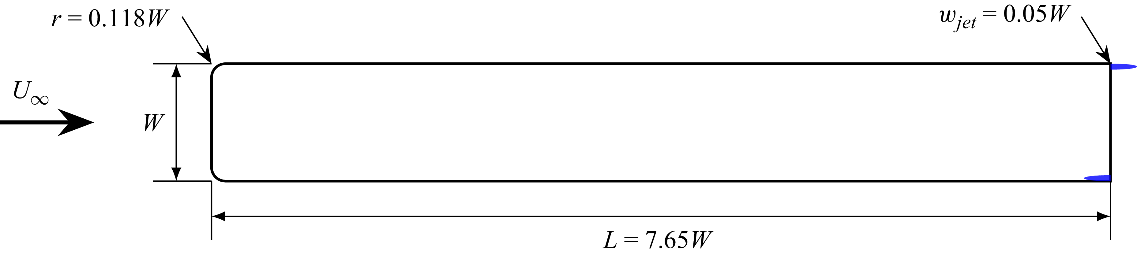

 Ux

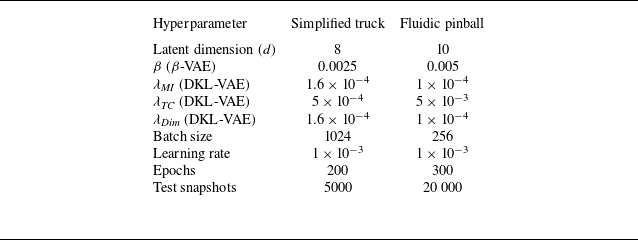
 β
 β
 β
 λMI
 λTC
 λDim

 t
 zt+1
 z˙t
 zt+1
 t+H
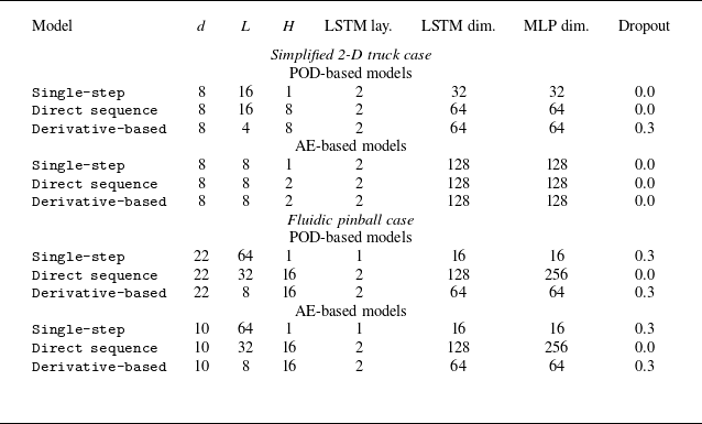

 τ=20
 τ=50
 β

 E
 E
 τ
 tc
 β
 E
 τ=0.1
 τ=5
 ∘
 ◊
 τ=0.1

 E
 E
 τ
 τ=50
 E
 τ=0.2
 τ=30
 τ=0.2

 β
 β

 L2
 eu2+ev2
 ei=⟨(u^i−ui)2⟩/σi2
 σi2
 τ∈[0,20]
 τ∈[0,100]
 β

 (z1∗,z2∗)
 β
 β

 (z2∗,z3∗)
 z1∗=0

 |Δϕ|
 |ΔA|
 β

 ⟨lnd(t)⟩
 β
 [3,10]tc
 [0.2,10]tc
 λref
 λpred
 λeff

 E=90%
 Δt
 2Δt
 4Δt
 E
 τ
 E
 ∘
 ◊

 St=fLref/U∞
 z1
 z4
 Lref
 U∞
 β

 E=80%
 90%
 95%
 E
 τ
 E
 ∘
 ◊

 E(τ)
 E
 τ=0.1
 τ=5
 22
 1
 β
 d=10
 1
 tanh
 1

 E=90%
 E
 τ
 E
 ∘
 ◊

 E
 τ
 E
 ∘
 ◊

 Open access

