1 Introduction
The horizontal component,
 $f_{H}$
, of the Coriolis vector is usually neglected in large-scale atmospheric–oceanographic modelling under the ‘traditional approximation’ as called by Eckart (Reference Eckart1960). Standard textbooks (e.g. Pedlosky Reference Pedlosky1987; Holton Reference Holton2004) suggest this approximation is justifiable. However, a robust demonstration was, to the best of our knowledge, never provided.
In recent years, interest in the potential critical role of
 $f_{H}$
in geophysical flows (the atmosphere–ocean system) has gradually developed, as reviewed by Gerkema et al. (Reference Gerkema, Zimmerman, Maas and van Haren2008). Among others, Thuburn, Wood & Staniforth (Reference Thuburn, Wood and Staniforth2002), Kasahara (Reference Kasahara2003a
,Reference Kasahara
b
, Reference Kasahara2007, Reference Kasahara2009), Gerkema & Shrira (Reference Gerkema and Shrira2005), Reznik (Reference Reznik2013, Reference Reznik2015) focus on the linear wave dynamics on the
 $f$
-plane. Glazunov (Reference Glazunov2010), for example, further considers the effects of friction in the boundary layer. Dellar & Salmon (Reference Dellar and Salmon2005), Dellar (Reference Dellar2011) examine the Hamiltonian structure of the problem.
The tropics is a particular area of interest, because the vertical component,
 $f_{v}$
, of the Coriolis vector vanishes at the equator, thus the horizontal component,
 $f_{H}$
, is more likely to play a critical role (Colin de Verdière & Schopp Reference Colin de Verdière and Schopp1994; White & Bromley Reference White and Bromley1995; Schopp & Colin de Verdière Reference Schopp and Colin de Verdière1997; Fruman Reference Fruman2009; Stewart & Dellar Reference Stewart and Dellar2011a
,Reference Stewart and Dellar
b
, Reference Stewart and Dellar2012; Hayashi & Itoh Reference Hayashi and Itoh2012). A special category of the problem intensively investigated, especially in the oceanographic context, is axisymmetrical equatorial circulations in the presence of
 $f_{H}$
(Stern Reference Stern1963; Stewartson Reference Stewartson1971, Reference Stewartson1972; Harlander & Maas Reference Harlander and Maas2007; Maas & Harlander Reference Maas and Harlander2007). However, a full three-dimensional analysis of the problem on a generalized equatorial
 $\unicode[STIX]{x1D6FD}$
-plane turns out to be complex, especially when the vertical boundary conditions of the system are properly taken into account (cf. Fruman Reference Fruman2009).
For this reason, the present paper focuses on the local analysis of a generalized
 $f$
-plane system by following Kasahara (Reference Kasahara2003a
,Reference Kasahara
b
) and Gerkema & Shrira (Reference Gerkema and Shrira2005). The focus here is on the low wavenumber limit. This is in contrast to the ray tracing method within a global rotating fluid – another promising direction of research (Rabitti & Maas Reference Rabitti and Maas2013, Reference Rabitti and Maas2014 and references therein) – in which the focus is on the high wavenumber limit.
The wave dynamics is not the only fundamental aspect to be investigated. The modifications of shear-instability problems by the full Coriolis force are considered by Tort, Ribstein & Zeitlin (Reference Tort, Ribstein and Zeitlin2016). The geostrophic-adjustment problem is addressed by Reznik (Reference Reznik2014a ,Reference Reznik b ). In contrast, the present study focuses on the wave dynamics.
The main motivation for the study stems from Gerkema & Shrira (Reference Gerkema and Shrira2005), who point out a drastic difference in linear wave dispersion curves in the large-scale limit with and without the ‘traditional approximation’, against an intuitive anticipation. They suggest (in their abstract) that the effect of the horizontal Coriolis component,
 $f_{H}$
, acts as a singular perturbation. However, the exact nature of this singularity is left to be identified in their study. The goal of the present paper is to actually examine this singular perturbation caused by the horizontal Coriolis component,
 $f_{H}$
, in the large-scale limit.
The paper is constructed as follows. The next section reviews the conventional wisdom that the horizontal Coriolis component,
 $f_{H}$
, is negligible in the large-scale limit by presenting a non-dimensionalized set of the system. The full linear dispersion relationships examined by Kasahara (Reference Kasahara2003a
) and Gerkema & Shrira (Reference Gerkema and Shrira2005) are reviewed in § 3. A perturbation analysis is developed in § 4. The paper is concluded by further discussions in § 5.
2 Equation system
For analysis, we take the linearized rotating Euler system in the Boussinesq approximation:
 $$\begin{eqnarray}\displaystyle & \displaystyle \frac{\unicode[STIX]{x2202}u}{\unicode[STIX]{x2202}t}-f_{v}v+f_{H}w+\frac{\unicode[STIX]{x2202}\unicode[STIX]{x1D719}}{\unicode[STIX]{x2202}x}=0, & \displaystyle\end{eqnarray}$$
 $$\begin{eqnarray}\displaystyle & \displaystyle \frac{\unicode[STIX]{x2202}v}{\unicode[STIX]{x2202}t}+f_{v}u+\frac{\unicode[STIX]{x2202}\unicode[STIX]{x1D719}}{\unicode[STIX]{x2202}y}=0, & \displaystyle\end{eqnarray}$$
 $$\begin{eqnarray}\displaystyle & \displaystyle \frac{\unicode[STIX]{x2202}w}{\unicode[STIX]{x2202}t}-f_{H}u+\frac{\unicode[STIX]{x2202}\unicode[STIX]{x1D719}}{\unicode[STIX]{x2202}z}=b, & \displaystyle\end{eqnarray}$$
 $$\begin{eqnarray}\displaystyle & \displaystyle \frac{\unicode[STIX]{x2202}u}{\unicode[STIX]{x2202}x}+\frac{\unicode[STIX]{x2202}v}{\unicode[STIX]{x2202}y}+\frac{\unicode[STIX]{x2202}w}{\unicode[STIX]{x2202}z}=0, & \displaystyle\end{eqnarray}$$
 $$\begin{eqnarray}\displaystyle & \displaystyle \frac{\unicode[STIX]{x2202}b}{\unicode[STIX]{x2202}t}+N^{2}w=0. & \displaystyle\end{eqnarray}$$
 $u$
,
 $v$
and
 $w$
are the eastward, northward and vertical components of the velocity;
 $\unicode[STIX]{x1D719}$
is a geopotential;
 $b$
the buoyancy (in unit of the acceleration of the gravity);
 $f_{v}=2\unicode[STIX]{x1D6FA}\sin \unicode[STIX]{x1D711}$
,
 $f_{H}=2\unicode[STIX]{x1D6FA}\cos \unicode[STIX]{x1D711}$
are the vertical and the horizontal components of the Coriolis vector, respectively, at the latitude,
 $\unicode[STIX]{x1D711}$
;
 $\unicode[STIX]{x1D6FA}$
is the planetary angular velocity;
 $N$
is the Brunt–Väisälä frequency. The coordinates,
 $(x,y,z)$
, are taken eastwards, northwards and upwards. No hydrostatic balance is assumed here for generality. By taking the so-called
 $f$
-plane approximation, the Coriolis vector,
 $(f_{H},f_{v})$
, is taken constant in the following. We assume a geometry of the system flat rigid lid at both bottom and top so that the vertical velocity vanishes. Recall that under the ‘traditional approximation’ (Eckart Reference Eckart1960), the horizontal component of the Coriolis vector is neglected by setting
 $f_{H}=0$
.
Non-dimensionalization is the most straightforward way of seeing the expected orders of magnitudes of the terms in a system so that a justification for neglecting the terms with
 $f_{H}$
can also be seen. The system (2.1a
)–(2.1e
) can be non-dimensionalized by setting
 $\unicode[STIX]{x2202}/\unicode[STIX]{x2202}t=f_{v}\unicode[STIX]{x2202}/\unicode[STIX]{x2202}t^{\ast }$
,
 $\unicode[STIX]{x2202}/\unicode[STIX]{x2202}x=(1/L)\unicode[STIX]{x2202}/\unicode[STIX]{x2202}x^{\ast }$
,
 $\unicode[STIX]{x2202}/\unicode[STIX]{x2202}z=(1/D)\unicode[STIX]{x2202}/\unicode[STIX]{x2202}z^{\ast }$
,
 $\boldsymbol{u}_{H}=U\boldsymbol{u}_{H}^{\ast }$
,
 $w=(D/L)Uw^{\ast }$
,
 $\unicode[STIX]{x1D719}=Lf_{v}U\unicode[STIX]{x1D719}^{\ast }$
,
 $b=(N^{2}/f_{v})(D/L)Ub^{\ast }$
. Here, typical spatial scales in the horizontal and vertical are
 $L$
and
 $D$
, respectively. A typical horizontal scale for the velocity is set
 $U$
and
 $^{\ast }$
is added to indicate the non-dimensional variables.
After non-dimensinalization, we obtain
 $$\begin{eqnarray}\displaystyle & \displaystyle \frac{\unicode[STIX]{x2202}u}{\unicode[STIX]{x2202}t}-v+\unicode[STIX]{x1D6FC}\hat{f}_{H}w+\frac{\unicode[STIX]{x2202}\unicode[STIX]{x1D719}}{\unicode[STIX]{x2202}x}=0, & \displaystyle\end{eqnarray}$$
 $$\begin{eqnarray}\displaystyle & \displaystyle \frac{\unicode[STIX]{x2202}v}{\unicode[STIX]{x2202}t}+u+\frac{\unicode[STIX]{x2202}\unicode[STIX]{x1D719}}{\unicode[STIX]{x2202}y}=0, & \displaystyle\end{eqnarray}$$
 $$\begin{eqnarray}\displaystyle & \displaystyle \unicode[STIX]{x1D6FC}^{2}\frac{\unicode[STIX]{x2202}w}{\unicode[STIX]{x2202}t}-\unicode[STIX]{x1D6FC}\hat{f}_{H}u+\frac{\unicode[STIX]{x2202}\unicode[STIX]{x1D719}}{\unicode[STIX]{x2202}z}=\hat{F}b, & \displaystyle\end{eqnarray}$$
 $$\begin{eqnarray}\displaystyle & \displaystyle \frac{\unicode[STIX]{x2202}u}{\unicode[STIX]{x2202}x}+\frac{\unicode[STIX]{x2202}v}{\unicode[STIX]{x2202}y}+\frac{\unicode[STIX]{x2202}w}{\unicode[STIX]{x2202}z}=0, & \displaystyle\end{eqnarray}$$
 $$\begin{eqnarray}\displaystyle & \displaystyle \frac{\unicode[STIX]{x2202}b}{\unicode[STIX]{x2202}t}+\hat{N}^{2}w=0, & \displaystyle\end{eqnarray}$$
 $^{\ast }$
from the final results.
In presenting the system in non-dimensional form, the following non-dimensionalized parameters have been introduced:
 $\unicode[STIX]{x1D6FC}=D/L$
: aspect ratio,
 $\hat{F}=(L_{R}/L)^{2}$
: Froude number,
 $\hat{f}_{H}=f_{H}/f_{v}$
: ratio of the horizontal to the vertical component of the Coriolis vector,
 $\hat{N}=N/N_{0}$
: non-dimensionalized Brunt–Väisälä frequency.
Recall that the Rossby radius of deformation is defined by
 $$\begin{eqnarray}L_{R}=N_{0}D/f_{v}.\end{eqnarray}$$
Non-dimensionalized Brunt–Väisälä frequency,
 $\hat{N}$
, with a reference value,
 $N_{0}$
, is retained for now for allowing for the possibility of height dependence. Reznik (Reference Reznik2013, Reference Reznik2015) explicitly considers the height dependence of
 $\hat{N}$
. On the other hand, this parameter will simply be set to
 $\hat{N}=1$
for ease of analysis in the following sections. (Note that, in the equatorial limit,
 $f_{v}\rightarrow 0$
, the parameters
 $\hat{f}_{H}$
,
 $\hat{F}$
and
 $L_{R}$
diverge. However, this is not going to be an issue in the following by assuming a finite
 $f_{v}$
throughout.)
We see immediately from the above set (2.2a
)–(2.2e
) that the ‘traditional approximation’ is justified when the aspect ratio is small enough i.e.
 $\unicode[STIX]{x1D6FC}\ll 1$
, because the terms with
 $f_{H}$
are only of order
 $O(\unicode[STIX]{x1D6FC})$
. This is essentially a standard argument found in textbooks in order to justify the ‘traditional approximation’. A systematic analysis of other various limiting cases is provided by Reznik (Reference Reznik2013).
Importantly, having a small order of magnitude after non-dimensionalization for a given term is not always a sufficient reason for dropping it. A good example is the quasi-geostrophic approximation. In the terminology of asymptotic expansions the leading-order system is degenerate (cf. Greenspan Reference Greenspan1968) in this case. Thus we need to proceed to a higher order. As a result, some of the terms neglected at leading order must be considered explicitly.
3 Full dispersion relationship
A full dispersion relationship of the system (2.2a
)–(2.2e
) can be derived analytically, as presented in Kasahara (Reference Kasahara2003a
,Reference Kasahara
b
) and Gerkema & Shrira (Reference Gerkema and Shrira2005). In this section we set
 $\unicode[STIX]{x1D6FC}=1$
without loss of generality. Note that under this setting, the limit
 $\unicode[STIX]{x1D6FC}\rightarrow 0$
, considered in the next section, becomes equivalent to taking the limit
 $K\rightarrow 0$
.
The frequency,
 $\unicode[STIX]{x1D70E}$
, without the ‘traditional approximation’ is determined by
 $$\begin{eqnarray}\unicode[STIX]{x1D70E}^{2}=\frac{K^{2}(1+\tilde{f}_{H}^{2}+\hat{F})+2\tilde{m}^{2}}{2(K^{2}+\tilde{m}^{2})}\pm \frac{K^{2}(1-\hat{F})}{2(K^{2}+\tilde{m}^{2})}\{1+\unicode[STIX]{x1D706}_{1}\tilde{f}_{H}^{2}(1+\unicode[STIX]{x1D706}_{2}\tilde{f}_{H}^{2})\}^{1/2},\end{eqnarray}$$
where
 $$\begin{eqnarray}\displaystyle & \tilde{f}_{H}=(l/K)\hat{f}_{H}, & \displaystyle\end{eqnarray}$$
 $$\begin{eqnarray}\displaystyle & \displaystyle \unicode[STIX]{x1D706}_{1}=\frac{2}{(1-\hat{F})^{2}}\left(1+\hat{F}+\frac{2\tilde{m}^{2}}{K^{2}}\right), & \displaystyle\end{eqnarray}$$
 $$\begin{eqnarray}\displaystyle & \displaystyle \unicode[STIX]{x1D706}_{2}=\frac{1}{2(1+\hat{F})+4\tilde{m}^{2}/K^{2}}, & \displaystyle\end{eqnarray}$$
 $K$
is the total horizontal wavenumber,
 $\tilde{m}$
is the vertical wavenumber (‘standing component’ to be defined by (4.17) below) and
 $l$
is the latitudinal wavenumber.
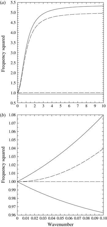
The numerical results are presented in figure 1 with
 $\hat{F}=5$
and
 $\tilde{f}_{H}^{2}=0.3$
. Here, figure 1(a) focuses on the large wavenumber limit, whereas figure 1(b) on the small wavenumber limit.
Full dispersion relationships (solid) obtained from the system (2.2a
)–(2.2e
) without ‘traditional approximation’ to be compared with the results (long-dash) under the ‘traditional approximation’. The square
 $\unicode[STIX]{x1D70E}^{2}$
of the frequency is shown as a function of the horizontal wavenumber,
 $K/\tilde{m}$
, normalized by the vertical wavenumber,
 $\tilde{m}$
, introduced by (4.17) later. The upper long-dash curve is the inertio-gravity wave under the ‘traditional approximation’, and the adjacent solid curve shows the modification by adding the horizontal component,
 $f_{H}$
, of the Coriolis vector. The lower long-dash line is the inertial oscillation solution obtained under the ‘traditional approximation’, and the adjacent solid curve is a modification by adding the terms with
 $f_{H}$
. The latter solution is called the boundary-induced inertial mode by Kasahara (Reference Kasahara2003a
). The parameter choices are:
 $\unicode[STIX]{x1D6FC}=1$
,
 $\hat{F}=5$
, and
 $\tilde{f}_{H}^{2}=0.3$
: (a) focuses on the large wavenumber limit, whereas (b) on the small wavenumber limit.

Figure 1(a) simply confirms the point that in the limit
 $K\rightarrow \infty$
(i.e.
 $\unicode[STIX]{x1D6FC}\rightarrow \infty$
), the contribution of
 $f_{H}$
certainly becomes important, as seen by gradual divergence of the two curves with and without ‘traditional approximation’. However, it may be worthwhile to note that the divergence begins already at a relatively small wavenumber (i.e.
 $K/\tilde{m}\sim 1$
, or
 $\unicode[STIX]{x1D6FC}\sim 1$
).
Figure 1(b) zooming in on the limit
 $K\rightarrow 0$
has one more surprise, because in the limit of small aspect ratio,
 $K\rightarrow 0$
(i.e.
 $\unicode[STIX]{x1D6FC}\rightarrow 0$
), as suggested by the equation set, (2.2a
)–(2.2e
), the contribution of
 $f_{H}$
would be negligible. However, the two curves with and without the ‘traditional approximation’ clearly follow different slopes,
 $\unicode[STIX]{x2202}\unicode[STIX]{x1D70E}^{2}/\unicode[STIX]{x2202}K$
in the limit
 $K\rightarrow 0$
against this prediction. As suggested by Gerkema & Shrira (Reference Gerkema and Shrira2005), there is a certain singular perturbation involved. The goal of the next section is to examine this issue in depth.
Finally, note that, as rather trivially observed in the figure, all the wave modes merge to the inertial oscillation in the limit of
 $K\rightarrow 0$
, as emphasized by Reznik (Reference Reznik2013, Reference Reznik2015). This simple fact turns out to be the key for resolving an apparent singularity of the system as
 $K\rightarrow 0$
in the next section.
However, before concluding the section, we present a simple analysis of the full dispersion relationship that gives a glimpse of the singularity of the problem. A possible singularity of the system is likely found in the square-root factor in the second term of (3.1). Thus, we attempt a Taylor expansion of this square-root factor in
 $\tilde{f}_{H}$
:
 $$\begin{eqnarray}\displaystyle \{1+\unicode[STIX]{x1D706}_{1}\tilde{f}_{H}^{2}(1+\unicode[STIX]{x1D706}_{2}\tilde{f}_{H}^{2})\}^{1/2} & = & \displaystyle 1+\frac{\tilde{f}_{H}^{2}}{(1-\hat{F})^{2}}\left(1+\hat{F}+\frac{2m^{2}}{K^{2}}\right)(1+\unicode[STIX]{x1D706}_{2}\tilde{f}_{H}^{2})\nonumber\\ \displaystyle & & \displaystyle -\,\frac{\tilde{f}_{H}^{4}}{2(1-\hat{F})^{4}}\left(1+\hat{F}+\frac{2m^{2}}{K^{2}}\right)^{2}(1+\unicode[STIX]{x1D706}_{2}\tilde{f}_{H}^{2})^{2}\nonumber\\ \displaystyle & & \displaystyle +\,\frac{\tilde{f}_{H}^{6}}{2(1-\hat{F})^{6}}\left(1+\hat{F}+\frac{2m^{2}}{K^{2}}\right)^{3}(1+\unicode[STIX]{x1D706}_{2}\tilde{f}_{H}^{2})^{3}-\cdots .\qquad\end{eqnarray}$$
This Taylor expansion diverges as
 $K\rightarrow 0$
, although the full expression for this square-root factor, multiplied by
 $K^{2}$
, is regular in this limit. This does not constitute any paradox, recalling that the Taylor expansion does not always work. However, it proves the simple point that
 $\tilde{f}_{H}$
cannot be treated as a small parameter in the limit of
 $K\rightarrow 0$
.
4 Singular perturbation analysis
In order to examine the behaviour of the system towards the large scale, we now take the limit
 $\unicode[STIX]{x1D6FC}\rightarrow 0$
in (2.2a
)–(2.2e
). We then perform the asymptotic expansion of the variables in
 $\unicode[STIX]{x1D6FC}$
, e.g.
 $$\begin{eqnarray}u=u^{(0)}+\unicode[STIX]{x1D6FC}u^{(1)}+\cdots .\end{eqnarray}$$
Similarly, we take an asymptotic expansion of the frequency in the same form, i.e.
 $$\begin{eqnarray}\unicode[STIX]{x1D70E}=\unicode[STIX]{x1D70E}^{(0)}+\unicode[STIX]{x1D6FC}\unicode[STIX]{x1D70E}^{(1)}+\cdots .\end{eqnarray}$$
Furthermore, note also that
 $\hat{F}\rightarrow 0$
in this limit, thus the relative orders of these two non-dimensional parameters must be specified, as discussed below.
Regardless of this choice, to leading order,
 $O(1)$
, we obtain:
 $$\begin{eqnarray}\displaystyle & \displaystyle \frac{\unicode[STIX]{x2202}u^{(0)}}{\unicode[STIX]{x2202}t}-v^{(0)}+\frac{\unicode[STIX]{x2202}\unicode[STIX]{x1D719}^{(0)}}{\unicode[STIX]{x2202}x}=0, & \displaystyle\end{eqnarray}$$
 $$\begin{eqnarray}\displaystyle & \displaystyle \frac{\unicode[STIX]{x2202}v^{(0)}}{\unicode[STIX]{x2202}t}+u^{(0)}+\frac{\unicode[STIX]{x2202}\unicode[STIX]{x1D719}^{(0)}}{\unicode[STIX]{x2202}y}=0, & \displaystyle\end{eqnarray}$$
 $$\begin{eqnarray}\displaystyle & \displaystyle \frac{\unicode[STIX]{x2202}\unicode[STIX]{x1D719}^{(0)}}{\unicode[STIX]{x2202}z}=0 & \displaystyle\end{eqnarray}$$
 $$\begin{eqnarray}\unicode[STIX]{x1D719}^{(0)}=0,\end{eqnarray}$$
and its substitution into the first two equations leads to:
 $$\begin{eqnarray}\displaystyle & \displaystyle \frac{\unicode[STIX]{x2202}u^{(0)}}{\unicode[STIX]{x2202}t}-v^{(0)}=0, & \displaystyle\end{eqnarray}$$
 $$\begin{eqnarray}\displaystyle & \displaystyle \frac{\unicode[STIX]{x2202}v^{(0)}}{\unicode[STIX]{x2202}t}+u^{(0)}=0 & \displaystyle\end{eqnarray}$$
or
 $$\begin{eqnarray}\displaystyle & \displaystyle \text{i}\unicode[STIX]{x1D70E}^{(0)}u^{(0)}-v^{(0)}=0, & \displaystyle\end{eqnarray}$$
 $$\begin{eqnarray}\displaystyle & \displaystyle \text{i}\unicode[STIX]{x1D70E}^{(0)}v^{(0)}+u^{(0)}=0. & \displaystyle\end{eqnarray}$$
 $\unicode[STIX]{x2202}\unicode[STIX]{x1D719}^{(0)}/\unicode[STIX]{x2202}z=0$
and
 $\unicode[STIX]{x1D719}^{(0)}\not =0$
does not lead to any wave solutions under the flat rigid lid top and bottom boundary conditions. The leading-order solution constitutes a pure inertial oscillation, and it immediately follows that
 $$\begin{eqnarray}\unicode[STIX]{x1D70E}^{(0)2}=1\end{eqnarray}$$
(cf. (2.10), Reznik Reference Reznik2013).
This solution is degenerate in the similar sense as the geostrophy. In this case, a horizontal structure of the solution is left undetermined. Thus, we need to proceed to a higher order in order to resolve this degeneracy.
4.1 The case with
 $\hat{F}\sim \unicode[STIX]{x1D6FC}$

In order to proceed to
 $O(\unicode[STIX]{x1D6FC})$
, we also need to set an order of
 $\hat{F}$
with respect to
 $\unicode[STIX]{x1D6FC}$
. There are two major possibilities: (i)
 $\hat{F}\sim \unicode[STIX]{x1D6FC}$
and (ii)
 $\hat{F}\sim \unicode[STIX]{x1D6FC}^{2}$
. These asymptotes amount to assuming
 $LD\sim$
constant and
 $D\sim \text{constant}$
, respectively, also assuming
 $L_{R}$
is a fixed parameter, as taking the limit
 $L\rightarrow \infty$
. The first possibility is considered in this subsection and the second in the next subsection.
Expecting
 $\hat{F}\sim \unicode[STIX]{x1D6FC}$
, we let
 $\hat{F}=\unicode[STIX]{x1D6FC}\tilde{F}$
for now. The main goal next is to define a correction,
 $\unicode[STIX]{x1D70E}^{(1)}$
, to the frequency along with a horizontal structure of the solution at
 $O(\unicode[STIX]{x1D6FC})$
. At this order, we obtain
 $$\begin{eqnarray}\displaystyle & \displaystyle \text{i}\unicode[STIX]{x1D70E}^{(0)}u^{(1)}-v^{(1)}+\text{i}\unicode[STIX]{x1D70E}^{(1)}u^{(0)}+\hat{f}_{H}w^{(0)}+\frac{\unicode[STIX]{x2202}\unicode[STIX]{x1D719}^{(1)}}{\unicode[STIX]{x2202}x}=0, & \displaystyle\end{eqnarray}$$
 $$\begin{eqnarray}\displaystyle & \displaystyle \text{i}\unicode[STIX]{x1D70E}^{(0)}v^{(1)}+u^{(1)}+\text{i}\unicode[STIX]{x1D70E}^{(1)}v^{(0)}+\frac{\unicode[STIX]{x2202}\unicode[STIX]{x1D719}^{(1)}}{\unicode[STIX]{x2202}y}=0, & \displaystyle\end{eqnarray}$$
 $$\begin{eqnarray}\displaystyle & \displaystyle -\hat{f}_{H}u^{(0)}+\frac{\unicode[STIX]{x2202}\unicode[STIX]{x1D719}^{(1)}}{\unicode[STIX]{x2202}z}=\tilde{F}b^{(0)}, & \displaystyle\end{eqnarray}$$
 $$\begin{eqnarray}\displaystyle & \displaystyle \frac{\unicode[STIX]{x2202}u^{(0)}}{\unicode[STIX]{x2202}x}+\frac{\unicode[STIX]{x2202}v^{(0)}}{\unicode[STIX]{x2202}y}+\frac{\unicode[STIX]{x2202}w^{(0)}}{\unicode[STIX]{x2202}z}=0, & \displaystyle\end{eqnarray}$$
 $$\begin{eqnarray}\displaystyle & \displaystyle \text{i}\unicode[STIX]{x1D70E}^{(0)}b^{(0)}+\hat{N}^{2}w^{(0)}=0. & \displaystyle\end{eqnarray}$$
 ${\sim}\text{exp}(\text{i}kx+\text{i}ly+\text{i}mz)$
. Note that
 $w^{(0)}$
and
 $\unicode[STIX]{x1D719}^{(1)}$
can be expressed in terms of
 $u^{(0)}$
and
 $v^{(0)}$
by using (4.9c
)–(4.9e
). By substituting these expressions into (4.9a
) and (4.9b
), we obtain a system in the form:
 $$\begin{eqnarray}\boldsymbol{L}^{(\mathbf{0})}\boldsymbol{q}^{(1)}+\boldsymbol{L}^{(\mathbf{1})}\boldsymbol{q}^{(0)}=0,\end{eqnarray}$$
where
 $\boldsymbol{q}^{(1)}=(u^{(1)},v^{(1)})$
,
 $\boldsymbol{q}^{(0)}=(u^{(0)},v^{(0)})$
;
 $\boldsymbol{L}^{(\mathbf{0})}$
and
 $\boldsymbol{L}^{(\mathbf{1})}$
are the leading-order and the first-order operators. The above equation physically means that the first-order variables,
 $\boldsymbol{q}^{(1)}$
, oscillate with the inertial period under a perturbation forcing due to the leading-order modulation, which is given by the second term. In order for the system to be well behaved, the forcing term should not cause a resonance to the first-order oscillation. This condition is mathematically called the solvability condition.
Generally speaking, this condition is obtained by multiplying the adjoint solution,
 $\boldsymbol{q}^{\dagger }=(u^{\dagger },v^{\dagger })$
, with the above equation from the left-hand side. After some manipulations, we obtain
 $$\begin{eqnarray}[\boldsymbol{L}^{\dagger }\boldsymbol{q}^{\dagger }]\boldsymbol{\cdot }\boldsymbol{q}^{(1)}+\boldsymbol{q}^{\dagger }\boldsymbol{\cdot }[\boldsymbol{L}^{(\mathbf{1})}\boldsymbol{q}^{(0)}]=0.\end{eqnarray}$$
Here, by definition, the adjoint system constitutes
 $$\begin{eqnarray}\boldsymbol{L}^{\dagger }\boldsymbol{q}^{\dagger }=0.\end{eqnarray}$$
Thus, the solvability condition is given by
 $$\begin{eqnarray}\boldsymbol{q}^{\dagger }\boldsymbol{\cdot }[\boldsymbol{L}^{(\mathbf{1})}\boldsymbol{q}^{(0)}]=0.\end{eqnarray}$$
In the present case, the adjoint problem is given by
 $$\begin{eqnarray}\displaystyle & \displaystyle \text{i}\unicode[STIX]{x1D70E}^{(0)}u^{\dagger }+v^{\dagger }=0, & \displaystyle\end{eqnarray}$$
 $$\begin{eqnarray}\displaystyle & \displaystyle \text{i}\unicode[STIX]{x1D70E}^{(0)}v^{\dagger }-u^{\dagger }=0, & \displaystyle\end{eqnarray}$$
 $$\begin{eqnarray}m^{2}[\unicode[STIX]{x1D70E}^{2}]^{(1)}-2mK\tilde{f}_{H}-K^{2}\tilde{F}=0,\end{eqnarray}$$
where
 $K^{2}=k^{2}+l^{2}$
,
 $\tilde{f}_{H}=l\hat{f}_{H}/K$
, and
 $[\unicode[STIX]{x1D70E}^{2}]^{(1)}$
is the first-order correction to
 $\unicode[STIX]{x1D70E}^{2}$
, which is given by
 $$\begin{eqnarray}[\unicode[STIX]{x1D70E}^{2}]^{(1)}=2\unicode[STIX]{x1D70E}^{(0)}\unicode[STIX]{x1D70E}^{(1)}.\end{eqnarray}$$
Solving the above equation for
 $m$
, we obtain:
 $$\begin{eqnarray}m=\unicode[STIX]{x1D6E4}\pm \tilde{m},\quad \unicode[STIX]{x1D6E4}=\tilde{f}_{H}K/[\unicode[STIX]{x1D70E}^{2}]^{(1)},\end{eqnarray}$$
with the vertical velocity given by
 $$\begin{eqnarray}w=\sin \tilde{m}z\text{e}^{\text{i}kx+\text{i}ly+\text{i}\unicode[STIX]{x1D6E4}z},\end{eqnarray}$$
and
 $\tilde{m}$
is defined in such a manner that the boundary conditions,
 $w=0$
, at the top and bottom are satisfied. It transpires that the separation of
 $m$
into
 $\unicode[STIX]{x1D6E4}$
and
 $\tilde{m}$
stems from a need for satisfying the top and the bottom boundary conditions of the problem (Kasahara Reference Kasahara2003a
). We may call
 $\unicode[STIX]{x1D6E4}$
and
 $\tilde{m}$
the vertical wavenumbers for the propagating and the standing components, respectively, by considering the manner that two components contribute to the solution (cf. Durran & Bretherton Reference Durran and Bretherton2004).
Substitution of (4.17) back into (4.15) leads to:
 $$\begin{eqnarray}\tilde{m}^{2}[\unicode[STIX]{x1D70E}^{2}]^{(1)}-\tilde{F}K^{2}-\frac{\tilde{f}_{H}^{2}K^{2}}{[\unicode[STIX]{x1D70E}^{2}]^{(1)}}=0.\end{eqnarray}$$
By solving the above, we obtain:
 $$\begin{eqnarray}[\unicode[STIX]{x1D70E}^{2}]^{(1)}=\frac{K^{2}}{\tilde{m}^{2}}\left[\frac{\tilde{F}}{2}\pm \frac{1}{2}\left(\tilde{F}^{2}+\frac{4\tilde{m}^{2}\tilde{f}_{H}^{2}}{K^{2}}\right)^{1/2}\right].\end{eqnarray}$$
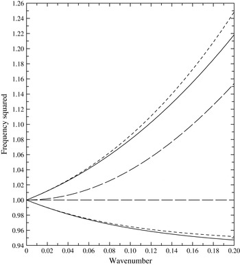
These two correction curves (4.20) are added as short-dashed curves in figure 2 on top of figure 1(b) but with the wavenumber range slightly modified. A fit of this leading-order correction (short-dashed) to the full solution (solid curves) is rather satisfactory, though we note a gradual tendency of the pairs to diverge towards the larger wavenumbers.
The same as figure 1(b) but with the leading-order corrections (assuming
 $\tilde{F}\sim \unicode[STIX]{x1D6FC}$
) added as short-dashed curves.

4.2 The case with
$\hat{F}\sim \unicode[STIX]{x1D6FC}^{2}$

Next, we proceed to the second possibility with
 $\hat{F}\sim \unicode[STIX]{x1D6FC}^{2}$
. In this case, we set
 $\hat{F}=\unicode[STIX]{x1D6FC}^{2}\tilde{F}$
. The procedure for this case works in analogous manner as in the previous case in the last subsection.
To
 $O(\unicode[STIX]{x1D6FC})$
, the problem is similar except the buoyancy term drops off by assuming a smaller Froude number,
 $\hat{F}$
, with respect to the aspect ratio,
 $\unicode[STIX]{x1D6FC}$
. Thus, the modulation of the solution to this order is purely due to the effect of the horizontal Coriolis component,
 $\hat{f}_{H}$
, and we obtain
 $$\begin{eqnarray}[\unicode[STIX]{x1D70E}^{2}]^{(1)}=\pm \frac{K}{\tilde{m}}\tilde{f}_{H}.\end{eqnarray}$$
The first-order correction,
 $[\unicode[STIX]{x1D70E}^{2}]^{(1)}$
, suggests how the waves should behave in purely inertial limit when the full Coriolis vector is considered.
We further proceed to
 $O(\unicode[STIX]{x1D6FC}^{2})$
, because we want to see a further modulation of the solution due to the buoyancy. Thus, the purely inertial oscillation to
 $O(\unicode[STIX]{x1D6FC})$
is modulated into the inertio-gravity wave to this order.
As it turns out, the analysis to this order is further involved by a need for taking into account a correction to the vertical wavenumber,
 $\unicode[STIX]{x1D6E4}$
, for the propagating component to
 $O(\unicode[STIX]{x1D6FC})$
. Thus,
 $\unicode[STIX]{x1D6E4}$
in (4.17b
) is replaced by
 $\unicode[STIX]{x1D6E4}+\unicode[STIX]{x1D6FC}\unicode[STIX]{x1D6E4}^{\prime }$
, and
 $$\begin{eqnarray}\unicode[STIX]{x1D6E4}^{\prime }=-\frac{\unicode[STIX]{x1D70E}^{(1)2}+2\unicode[STIX]{x1D70E}^{(0)}\unicode[STIX]{x1D70E}^{(2)}}{4\unicode[STIX]{x1D70E}^{(0)2}\unicode[STIX]{x1D70E}^{(1)2}}\tilde{f}_{H}K\end{eqnarray}$$
by referring to (2.25) of Kasahara (Reference Kasahara2003a ). By also taking account of this modification, we obtain
 $$\begin{eqnarray}[\unicode[STIX]{x1D70E}^{2}]^{(2)}=\frac{K^{2}}{2\tilde{m}^{2}}[\tilde{F}+\tilde{f}_{H}^{2}-1].\end{eqnarray}$$
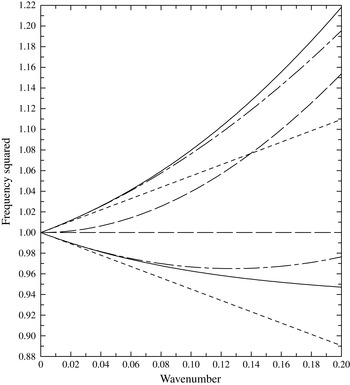
The obtained corrections are shown in figure 3. The full solutions are clearly asymptotic to the approximate solutions,
 $[\unicode[STIX]{x1D70E}^{2}]^{(1)}$
, to the limit of
 $K\rightarrow 0$
, although the departure is relatively fast as the wavenumber,
 $K$
, increases. The correction to the second order,
 $[\unicode[STIX]{x1D70E}^{2}]^{(2)}$
, adds the effect of the buoyancy to the first-order correction. Improvement of the solutions as a result is rather dramatic.
The same as figure 1(b) but the corrections under the assumption
 $\hat{F}\sim \unicode[STIX]{x1D6FC}^{2}$
to
 $O(\unicode[STIX]{x1D6FC})$
and
 $O(\unicode[STIX]{x1D6FC}^{2})$
and are, respectively, shown by the short-dashed and chain-dashed curves.

5 Discussion
Even the linear waves on a standard
 $f$
-plane may be considered a virtually singular problem. A standard deduction process of reducing the number of dependent variables assuming a waveform solution can easily lose the inertial oscillation as an additional solution. For example, the vertical normal-mode equation as given by (3.14) of Kasahara (Reference Kasahara2003a
) or (2) of Durran & Bretherton (Reference Durran and Bretherton2004) simply excludes the inertial-oscillation solution with
 $\unicode[STIX]{x1D70E}=f_{v}$
. Presumably due to this reason, figure 1(d) of Gerkema & Shrira (Reference Gerkema and Shrira2005) does not show the inertial oscillation as an additional solution. Note that its reproduction in figure 1(b) includes the inertial-oscillation solution.
The role of the horizontal Coriolis parameter,
 $f_{H}$
, may be considered to remove this virtual singularity. As a result, the solution of the pure inertial oscillation is lost, and it turns out into another inertio-gravity mode. Kasahara (Reference Kasahara2003a
) proposes to call this mode the boundary-induced inertial mode. At the same time, it leads to another singularity, that makes the wave solutions qualitatively different from those under the traditional approximation. The main goal of the present study has been to resolve this ‘non-traditional’ singularity to the system.
An important lesson to learn from the present analysis is a danger of relying on a simple scale analysis in order to decide whether a given term in a system can be neglected or not. We should keep in mind that such an analysis only provides a crude idea about the importance of the terms, and a final judgment is always left to a more careful analysis of the behaviour of the system. A linear analysis, as presented herein, is an important next step to take, due to its relative ease. Here, the importance of an ostensibly small term is revealed as a result. As stated by Reznik (Reference Reznik2013), ‘the non-traditional terms cause a dispersion of near-inertial oscillations’ in this limit.
In general, the most basic test would be to check whether a leading-order system obtained by a scale analysis can provide full information of a given system. In case of the present study, the leading-order inertial oscillation does not provide any information about the spatial structure of the solution. Thus, we need to proceed to a higher order. The situation is to some extent, analogous to the quasi-geostrophic problem. In both cases, the higher-order small terms become of critical importance as a result.
This kind of situation with a lack of full information to the solution is generally called degeneracy. Here, we encounter a rather semantic question: Gerkema & Shrira (Reference Gerkema and Shrira2005) have suggested that the limit
 $K\rightarrow 0$
for the wave problem on the generalized
 $f$
-plane constitutes a ‘singular perturbation’: however is it really a singular perturbation problem? In standard terminology, a singular perturbation constitutes a situation in which a term with a small parameter, ostensibly negligible, becomes important for a leading-order problem due to a high-order derivative associated with a given term (cf. § 7.2 Bender & Orszag Reference Bender and Orszag1978). The boundary layer is such a typical problem.
However, in the present case, no higher-order derivative is involved. Rather the degeneracy of the leading-order solution forces us to consider a contribution of small terms in order to close the problem. In this respect, the degeneracy may be considered a type of a singularity to a system, as in the present case, but in a sense different from conventional terminology.
More specifically, in order to resolve the degeneracy, the two possibilities for the asymptotic expansions are considered:
 $\hat{F}\sim \unicode[STIX]{x1D6FC}$
and
 $\hat{F}\sim \unicode[STIX]{x1D6FC}^{2}$
. Simple substitution of the definitions of the two non-dimensional parameters shows that the first case amounts to assuming
 $D/L_{R}\sim L_{R}/L$
, whereas the second is
 $D\sim L_{R}$
. In the Earth’s atmosphere, we usually have a situation with
 $D/L_{R}\ll 1$
, thus even the first case suggests an extremely large scale beyond the length of the great circle of the Earth. On the other hand, the deformation radius,
 $L_{R}$
, is relatively small in the oceans, and it is well possible to conceive a situation like the first case, and even the second case may be realizable when a sufficiently deep circulation is considered. In this respect, the singular behaviour of the wave dispersion in the large-scale limit arising from the horizontal component of the Coriolis vector is likely to be more important in ocean dynamics than in the atmosphere (cf. Kasahara Reference Kasahara2009).
To some extent, the second asymptotic expansion provides more insight in the full solutions. Note that, in both cases for the asymptotic expansion, the problem reduces to an asymptotic expansion of the square,
 $\unicode[STIX]{x1D70E}^{2}$
, of the frequency as
 $$\begin{eqnarray}\unicode[STIX]{x1D70E}^{2}=[\unicode[STIX]{x1D70E}^{2}]^{(0)}+\unicode[STIX]{x1D6FC}[\unicode[STIX]{x1D70E}^{2}]^{(1)}+\unicode[STIX]{x1D6FC}^{2}[\unicode[STIX]{x1D70E}^{2}]^{(2)}+\cdots .\end{eqnarray}$$
As it turns out, under the second asymptotic expansion, each term furthermore takes the form:
 $$\begin{eqnarray}[\unicode[STIX]{x1D70E}^{2}]^{(n)}=c_{n}K^{n}\end{eqnarray}$$
with
 $c_{n}$
constant with respect to
 $K$
for
 $n=0,1,\ldots .$
It transpires that essentially a Taylor expansion in wavenumber,
 $K$
, is developed under this asymptotic expansion.
On the other hand, the leading-order correction obtained with the first approach poses the same problem as results with the Taylor expansion of
 $\unicode[STIX]{x1D70E}^{2}$
in
 $\tilde{f}_{H}$
as pointed out by (3.3). This correction also leads to a similar divergent Taylor expansion in
 $K$
.
Here, the Froude number,
 $\hat{F}$
, plays an equally important role as the aspect ratio,
 $\unicode[STIX]{x1D6FC}$
, in this problem. Unfortunately, we do not see any clear transition of the dispersion in figure 1(b) by crossing the Rossby radius of deformation (i.e.
 $\hat{F}=1$
). For this reason, Gerkema & Shrira (Reference Gerkema and Shrira2005) even go on to argue that ‘the notion of the Rossby radius of deformation becomes invalid’. This is indeed true up to
 $O(K)$
as shown by (4.21) in § 4.2. However, its subtle role must clearly be emphasized in defining the wave dispersion to
 $O(K^{2})$
as shown by (4.23). These asymptotic behaviours are essentially consistent with the asymptotic behaviours as
 $K\rightarrow 0$
summarized by Reznik (Reference Reznik2013) by his equations (4.32) and (4.33). Reznik (Reference Reznik2013) further considers the wave evolution as an initial-value problem in this limit.
Acknowledgements
A main part of the present work is performed when I was a visiting scientist to NCAR during July–August 2015. A. Kasahara has effectively put me into a position of considering this problem. The work is performed under intensive discussions with him, and the manuscript has been scrutinized by him. Nevertheless, he restrains himself from being a co-author citing his health reasons. J. Tribbia has also provided me extensive suggestions.