3.1. Effect of the buoyancy Reynolds number

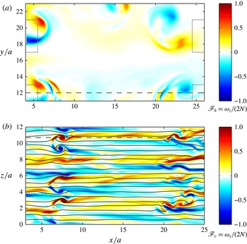
Figure 3 displays horizontal and vertical cross-sections of the flow for $F_{h}=0.85$ , $\mathscr{R}=1080$ ( $\mathscr{R}_{t}=0.81$ ) and for a time $t=475$ corresponding to the statistically stationary regime. Only a portion of the numerical box is shown to zoom in. The positions of four dipole generators are indicated by black rectangles. The colours in figure 3(a) represent the local horizontal Froude number defined as $\mathscr{F}_{h}={\it\omega}_{z}/(2N)$ , i.e. the vertical vorticity ${\it\omega}_{z}$ rescaled by $2N$ . The extrema of the local horizontal Froude number $\mathscr{F}_{h}$ corresponding to the large-scale vortices seen in figure 3(a) are of the same order as the horizontal Froude number $F_{h}=0.85$ confirming the equivalence between the local horizontal Froude number $\mathscr{F}_{h}$ and the Froude number $F_{h}$ based on the forced vortices. Large-scale vortices are seen only in the vicinity of the vortex generators. This is because they are destroyed by instabilities and interactions with the ambient flow before reaching the central part of the box as observed in the experiments. The nature of the small-scale structures visible on the sides of the horizontal cross-section in 3(a) can be understood by looking at the vertical cross-section in figure 3(b), where the isopycnals are plotted in black lines. We see overturnings of the isopycnals typical of the shear instability. In this figure, the colours correspond to the local vertical Froude number defined as $\mathscr{F}_{v}={\it\omega}_{y}/(2N)$ , where ${\it\omega}_{y}$ is the vorticity component normal to the view plane. This number compares locally the horizontal vorticity (which corresponds to the vertical gradients of horizontal velocity in strongly stratified flows) to the mean stratification. When the local density perturbations are neglected, this Froude number can be used to quantify approximately the local Richardson number:

(3.1) $$\begin{eqnarray}\mathit{Ri}=\frac{-(g/{\it\rho}_{0})(\partial {\it\rho}_{tot}/\partial z)}{|\partial \boldsymbol{u}_{h}/\partial z|^{2}}\lesssim \frac{1}{4\mathscr{F}_{v}^{2}}.\end{eqnarray}$$

This means that a value $\mathscr{F}_{v}=O(1)$ corresponds to a Richardson number of order $1/4$ , the critical value below which the shear instability can develop for an inviscid parallel stratified flow (Miles Reference Miles1961; Howard Reference Howard1961). We see that $|\mathscr{F}_{v}|$ is indeed high and of order unity in the regions where the overturnings of the isopycnals occur.

Figure 3.

Horizontal cross-section at $z/a=4$ (a) (only half the domain is shown), and vertical cross-section at $y/a=20$ (b) of the flow for $F_{h}=0.85$ and $\mathscr{R}=1080$ ( $\mathscr{R}_{t}=0.81$ ) and for a time $t=420$ corresponding to the statistically stationary regime. The contours represent the local horizontal Froude number $\mathscr{F}_{h}={\it\omega}_{z}/(2N)$ in (a) and the local vertical Froude number $\mathscr{F}_{v}={\it\omega}_{y}/(2N)$ in (b). The dashed horizontal lines indicate the location of the cross-section in the perpendicular direction. The black lines in (b) are isopycnals of total density with contour interval equal to 0.6. The grey boxes in (a) indicate the regions where the dipole forcing is impulsively applied.

We now turn to smaller values of the buoyancy Reynolds number corresponding to the values achieved in the experiments, where small-scale structures and overturnings were observed only for sufficiently high buoyancy Reynolds number. In order to investigate this point, figure 4 displays horizontal and vertical cross-sections of the flow as in figure 3 but for $\mathscr{R}=325$ ( $\mathscr{R}_{t}=0.28$ ), which corresponds to the highest buoyancy Reynolds number achieved in the experiments. Even if the turbulence is less intense, the isopycnals in figure 4(b) are clearly overturned by small billows in the regions where the local vertical Froude number $\mathscr{F}_{v}$ is of order unity. In the horizontal cross-section (figure 4 a), we see some small scales superimposed on the large-scale vortices. This confirms indirectly that the shear instability was operating in the experiments for the highest buoyancy Reynolds number achieved $\mathscr{R}=325$ ( $\mathscr{R}_{t}=0.28$ ).

Figure 4.

Same as figure 3 but for $F_{h}=0.85$ and $\mathscr{R}=325$ ( $\mathscr{R}_{t}=0.28$ ), i.e. for the values corresponding to the flow with the highest buoyancy Reynolds number achieved in the experiments. In (a) the half-domain shown is displaced compared with figure 3.

Figure 5.

(a) Transverse and longitudinal horizontal compensated second-order structure functions $S_{2T}(r_{r})$ (continuous lines) and $S_{2L}(r_{h})$ (dashed lines) for $F_{h}=0.85$ for different buoyancy Reynolds numbers given in the legend of (b). The inset in (a) shows the effective dimension $d_{eff}$ defined by (3.2). (b) Horizontal (continuous lines) and vertical (dashed lines) compensated one-dimensional spectra of kinetic energy $E_{K}(k_{i}){\it\varepsilon}_{\!K}^{-2/3}{k_{i}}^{5/3}$ for $F_{h}=0.85$ as a function of the scaled wavenumber $k_{i}/K$ , where $k_{i}$ denotes either the horizontal wavenumber $k_{h}$ or the vertical wavenumber $k_{z}$ . In (b), the horizontal black line corresponds to the $C_{1}{\it\varepsilon}_{\!K}^{2/3}{k_{i}}^{-5/3}$ law, with $C_{1}=0.5$ .

In the experimental study (Augier et al. Reference Augier, Billant, Negretti and Chomaz2014), the appearance of small scales has been quantified by measuring the horizontal transverse second-order structure function $S_{2T}(r_{h})=\langle [{\it\delta}u_{x}({\it\delta}y=r_{h})]^{2}+[{\it\delta}u_{y}({\it\delta}x=r_{h})]^{2}\rangle /2$ and the horizontal longitudinal second-order structure function $S_{2L}(r_{h})=\langle [{\it\delta}u_{x}({\it\delta}x=r_{h})]^{2}+[{\it\delta}u_{y}({\it\delta}y=r_{h})]^{2}\rangle /2$ , where ${\it\delta}u_{x}({\it\delta}y)=u_{x}(\boldsymbol{x}+{\it\delta}y\boldsymbol{e}_{\boldsymbol{y}})-u_{x}(\boldsymbol{x})$ is the transverse increment of $u_{x}$ , ${\it\delta}u_{x}({\it\delta}x)=u_{x}(\boldsymbol{x}+{\it\delta}x\boldsymbol{e}_{\boldsymbol{x}})-u_{x}(\boldsymbol{x})$ is the longitudinal increment of $u_{x}$ and the increments of $u_{y}$ are defined similarly. Figure 5(a) displays the compensated structure functions for four buoyancy Reynolds numbers in the range $86\leqslant \mathscr{R}\leqslant 2170$ for $F_{h}=0.85$ ( $0.09\leqslant \mathscr{R}_{t}\leqslant 1.46$ ). The increment $r_{h}$ is scaled by $R\equiv 4a$ , the characteristic length scale of the dipoles that are forced. The power law at the smaller scales correspond to a ${r_{h}}^{2}$ slope meaning that the dissipative range is resolved. An inertial range is associated with a structure function scaling like ${r_{h}}^{2/3}$ , i.e. a flat slope for the compensated structure functions. We do not see such an inertial range in figure 5(a) even if there is a flattening of the compensated structure functions at very large scales when the buoyancy Reynolds number increases. An increase of the energy at the small scales, especially for the transverse structure functions, can also be seen. This flattening was observed in the experimental study and was interpreted as the first indications of the inertial range that is predicted for large buoyancy Reynolds number. In order to interpret the difference between longitudinal and transverse structure functions, we consider a so-called effective dimension,

(3.2) $$\begin{eqnarray}d_{eff}(r_{h})=1+\frac{r_{h}(\partial S_{2L}/\partial r_{h})}{S_{2T}-S_{2L}}.\end{eqnarray}$$

This quantity is not a real dimension but is equal to 2 for a two-dimensional isotropic flow and to 3 for a three-dimensional isotropic flow, since the longitudinal and transverse second-order structure functions are related by

(3.3) $$\begin{eqnarray}S_{2T}(r)=\left(1+\frac{r}{d-1}\frac{\partial }{\partial r}\right)S_{2L}(r),\end{eqnarray}$$

where $d$ is the dimension of the space. As shown in the inset of figure 5(a), the effective dimension is very close to 2 at large scales for each buoyancy Reynolds number reflecting the fact that the forcing is two-dimensional. However for the highest value of the buoyancy Reynolds number, $d_{eff}(r_{h})$ increases at small scales to reach a value around 5 while it remains approximately equal to 2 for the lowest values of the buoyancy Reynolds number. Values of $d_{eff}$ larger than 3 were also observed in the experiments. They are related to the fact that the small-scale structures for these intermediate buoyancy Reynolds numbers are three-dimensional but still strongly anisotropic.

Figure 6.

Vertical (a,b) and horizontal (c,d) cross-sections of the velocity and local Froude number fields for $F_{h}=0.5$ , $\mathscr{R}=250$ ( $\mathscr{R}_{t}=0.21$ ) in (a,c) and for $F_{h}=2$ , $\mathscr{R}=1640$ ( $\mathscr{R}_{t}=1.8$ ) in (b,d).

In figure 5(b), the horizontal compensated one-dimensional spectra of kinetic energy $E_{K}(k_{h}){\it\varepsilon}_{\!K}^{-2/3}{k_{h}}^{5/3}$ is plotted as a function of the horizontal wavenumber $k_{h}$ scaled by $K=2{\rm\pi}/R$ , where $R\equiv 4a$ (for details on how the one-dimensional spectra are computed, see Augier et al. Reference Augier, Chomaz and Billant2012). The vertical compensated spectra $E_{K}(k_{z}){\it\varepsilon}_{\!K}^{-2/3}{k_{z}}^{5/3}$ is also shown with dashed lines. At horizontal wavenumbers around $K$ , the different horizontal spectra collapse. When the buoyancy Reynolds number is increased, we observe an increase of the spectra at large wavenumber $k_{h}>K$ and a decrease at low wavenumbers $k_{h}\ll K$ . This indicates that there is more transfers toward small scales and less transfers toward the largest scales. This is consistent with the interpretation of a transition from a regime dominated by viscous effects toward the strongly stratified turbulent regime when the buoyancy Reynolds number is increased. However, for buoyancy Reynolds number of the order of the largest value achieved in the experiments ( $\mathscr{R}=433$ , $\mathscr{R}_{t}=0.37$ , light thin line), the compensated spectra is not flat indicating that there is no inertial range for the typical range of parameters of the experiments. In contrast, the horizontal spectrum for the highest buoyancy Reynolds number $\mathscr{R}=2170$ ( $\mathscr{R}_{t}=1.46$ ) in figure 5(b) exhibits a $k_{h}^{-5/3}$ power law at wavenumbers slightly larger than $K$ . The horizontal black line indicates the $C_{1}{{\it\varepsilon}_{\!K}}^{2/3}{k_{h}}^{-5/3}$ law, with $C_{1}=0.5$ , which corresponds to the spectra of forced strongly stratified turbulence observed by Lindborg (Reference Lindborg2006) and Brethouwer et al. (Reference Brethouwer, Billant, Lindborg and Chomaz2007). We see that the kinetic energy spectrum for $\mathscr{R}=2170$ is close to this line suggesting that the flow approaches the strongly stratified turbulent regime. However, this regime is only incipient since the associated turbulent buoyancy Reynolds number is still only equal to $\mathscr{R}_{t}=1.46$ while Brethouwer et al. (Reference Brethouwer, Billant, Lindborg and Chomaz2007) showed that values larger than approximately 5 are necessary to really reach this regime. The compensated vertical spectrum (dashed lines in figure 5 b) strongly varies when the buoyancy Reynolds number is increased with more and more energy at small vertical scales. This confirms that for the smallest values of the buoyancy Reynolds number, vertical scales are controlled by dissipative effects. However, for $\mathscr{R}=1080$ ( $\mathscr{R}_{t}=0.81$ ) and $\mathscr{R}=2170$ ( $\mathscr{R}_{t}=1.46$ ), a peak in the compensated vertical spectra can be seen at approximately $k_{z}=1.5K$ . For both simulations, this wavenumber is not in the dissipative range in contrast to the simulations for the smaller values of the buoyancy Reynolds number, where no peak is observed. The appearance of the ${k_{h}}^{-5/3}$ power law in the horizontal spectra coincides with the appearance of this peak.

3.2. Effect of the Froude number $F_{h}$

The effect of the horizontal Froude number $F_{h}$ is addressed in figure 6. Vertical (a,b) and horizontal (c,d) cross-sections of the flow are presented for two different horizontal Froude numbers: $F_{h}=0.5$ (a,c) and $F_{h}=2$ (b,d) but for similar values of the quantity $\mathscr{R}^{\prime }=(\mathit{Re}-400){F_{h}}^{2}$ . The condition $\mathscr{R}^{\prime }>4$ should be satisfied to have the shear instability developing on a single columnar dipole affected by the zigzag instability (Augier & Billant Reference Augier and Billant2011). Here, it is approximately $\mathscr{R}^{\prime }\simeq 40$ like in the experiments for $\mathscr{R}=330$ . The local horizontal Froude number $\mathscr{F}_{h}={\it\omega}_{z}/(2N)$ (figure 6 c,d) has maximum values of the order of $F_{h}$ . In contrast, the local vertical Froude number $\mathscr{F}_{v}={\it\omega}_{y}/(2N)$ (figure 6 a,b) is of order unity. We see in figure 6(a) several rolls that are small compared with the horizontal scale of the vortices and seems to be due to the shear instability. Since $F_{h}=2$ corresponds to a weakly stratified flow, the maximum values of $|\mathscr{F}_{v}|$ are even higher than unity in figure 6(b). The rolls are in that case about the same size as the horizontal vortices.

3.3. Vertical structure

In order to quantify the variations with the buoyancy Reynolds number and the Froude number $F_{h}$ of the characteristic length scales of the flow, we have computed the characteristic vertical length scale $l_{v}=(2{U_{x}}^{2}/\langle [\partial _{z}u_{x}]^{2}\rangle )^{1/2}$ and horizontal length scale $l_{h}=(2{U_{x}}^{2}/\langle [\partial _{x}u_{x}]^{2}\rangle )^{1/2}$ , where $u_{x}$ is the velocity component in the $x$ direction and ${U_{x}}^{2}=\langle {u_{x}}^{2}\rangle$ . These scales are the equivalent of the Taylor micro-scale in isotropic turbulence. The evolution of the aspect ratio $l_{v}/l_{h}$ when the buoyancy Reynolds number is varied is shown in figure 7. Following Brethouwer et al. (Reference Brethouwer, Billant, Lindborg and Chomaz2007), two different scaling laws are tested: a viscous scaling law in figure 7(a) and an inviscid scaling law in figure 7(b). The viscous scaling law is obtained by balancing the dissipation due to vertical gradients and the horizontal advection $l_{v}\sim \sqrt{{\it\nu}l_{h}/U}\sim l_{h}/\sqrt{\mathit{Re}}$ (Godoy-Diana et al. Reference Godoy-Diana, Chomaz and Billant2004). The inviscid scaling law is obtained by balancing the buoyancy term to the vertical advection so that $l_{v}\sim U/N\sim l_{h}F_{h}$ (Billant & Chomaz Reference Billant and Chomaz2001). We see that the viscous scaling law works at low $\mathscr{R}\lesssim 250$ whereas the invicid scaling law is better at large buoyancy Reynolds number provided that $F_{h}\leqslant 1$ . It is consistent with the interpretation of a transition around $\mathscr{R}\approx 250$ from a viscous regime for which the vertical length scale is fixed by viscous effects (Godoy-Diana et al. Reference Godoy-Diana, Chomaz and Billant2004) to a nonlinear stratified regime for which the vertical length scale is fixed by an invariance of the hydrostatic Euler equations valid for strong stratification (Billant & Chomaz Reference Billant and Chomaz2001).

Figure 7.

Scaled aspect ratio (a) $(l_{v}/l_{h})\mathit{Re}^{1/2}$ and (b) $l_{v}/(l_{h}F_{h})$ as a function of $\mathscr{R}$ for different $F_{h}$ . The viscous and inviscid scaling laws $l_{v}/l_{h}\simeq 9.4\mathit{Re}^{-1/2}$ and $l_{v}/l_{h}\simeq 0.65F_{h}$ , where the constants are empiric, are plotted respectively with a dashed line and a dotted line. The oblique crosses $\times$ correspond to purely toroidal simulations, i.e. to the limit $F_{h}=0$ .

3.4. Spectral analyses of the simulation for $F_{h}=0.66$ and $\mathscr{R}=3560~(\mathscr{R}_{t}=2.4)$

3.4.1. Two-dimensional energy spectra

Figure 8 displays the compensated horizontal two-dimensional spectra as a function of ${\it\kappa}_{h}=({k_{x}}^{2}+{k_{y}}^{2})^{1/2}$ for $F_{h}=0.66$ and for $\mathscr{R}=3560$ ( $\mathscr{R}_{t}=2.4$ ), i.e. one of the highest buoyancy Reynolds number achieved with the forcing considered in this section (for precise definitions of two-dimensional spectra, see Augier et al. Reference Augier, Chomaz and Billant2012). The compensated horizontal two-dimensional kinetic spectrum $E_{K}({\it\kappa}_{h}){\it\varepsilon}_{\!K}^{-2/3}{\it\kappa}_{h}^{5/3}$ presents a ${\it\kappa}_{h}^{-5/3}$ power law at wavenumbers larger than $K$ . Remarkably, it approximately collapses on the horizontal line which indicates the $C_{2D}{\it\varepsilon}_{\!K}^{2/3}{{\it\kappa}_{h}}^{-5/3}$ law, with $C_{2D}=0.66$ corresponding to strongly stratified turbulence (Lindborg & Brethouwer Reference Lindborg and Brethouwer2007). The compensated horizontal two-dimensional potential spectrum $E_{P}({\it\kappa}_{h}){\it\varepsilon}_{\!K}^{-2/3}{\it\kappa}_{h}^{5/3}({\it\varepsilon}_{\!K}/{\it\varepsilon}_{\!P})$ also collapses on this line in agreement with Lindborg & Brethouwer (Reference Lindborg and Brethouwer2007). However, both kinetic and potential spectra exhibit a rebound at small scales as also observed by Brethouwer et al. (Reference Brethouwer, Billant, Lindborg and Chomaz2007).

Figure 8.

Compensated horizontal two-dimensional spectra (kinetic $E_{K}$ , potential $E_{P}$ , poloidal $E_{Kp}$ and toroidal $E_{Kt}$ ) as a function of ${\it\kappa}_{h}=|\boldsymbol{k}_{h}|$ for $F_{h}=0.66$ , $\mathscr{R}=3560$ corresponding to $\mathscr{R}_{t}=2.4$ . The black horizontal line shows the $C_{2D}{\it\varepsilon}_{\!K}^{2/3}{{\it\kappa}_{h}}^{-5/3}$ law, with $C_{2D}=0.66$ (Lindborg & Brethouwer Reference Lindborg and Brethouwer2007).

The toroidal spectrum $E_{Kt}$ , associated with rotational motions and the poloidal spectrum $E_{Kp}$ , associated with the vertical velocity and to the divergence of the horizontal velocity (Craya Reference Craya1958; Herring Reference Herring1974; Cambon Reference Cambon2001; Augier et al. Reference Augier, Chomaz and Billant2012) are also plotted in dashed and dash-dotted lines, respectively. Note that the toroidal and poloidal spectra cannot be simply associated with vortices or waves since their dynamics are intimately linked when $F_{v}\sim 1$ as pointed out by Billant & Chomaz (Reference Billant and Chomaz2001) and Lindborg & Brethouwer (Reference Lindborg and Brethouwer2007). At large scales, the toroidal spectrum dominates reflecting the rotational nature of the forcing by dipoles. The toroidal and poloidal spectra are of the same order in the inertial range as reported by Lindborg & Brethouwer (Reference Lindborg and Brethouwer2007). However, we can see that the poloidal spectrum is slightly larger than its toroidal counterpart as also observed by Waite (Reference Waite2011). This could be due to the shear instability since Kelvin–Helmholtz rolls with axis along the horizontal direction consist only in poloidal velocity. In any case, Lindborg & Brethouwer (Reference Lindborg and Brethouwer2007) have shown that such a high poloidal spectrum does not imply that the flow is dominated by waves. Indeed, a poloidal flow corresponds to linear waves only in the limit $F_{v}\ll 1$ .

3.4.2. Spectral energy budget: quantification of the direct energy cascade

The evolution equations of the kinetic and potential energies $\hat{E}_{K}(\boldsymbol{k})=|\hat{\boldsymbol{u}}|^{2}/2$ and $\hat{E}_{P}(\boldsymbol{k})=|\hat{{\it\rho}^{\prime }}|^{2}/(2{F_{h}}^{2})$ of a wavenumber $\boldsymbol{k}$ can be expressed as

(3.4) $$\begin{eqnarray}\displaystyle & \displaystyle \frac{\text{d}\hat{E}_{K}(\boldsymbol{k})}{\text{d}t}=\hat{T}_{K}-{\hat{C}}-\hat{D}_{K}+\hat{P}, & \displaystyle\end{eqnarray}$$

(3.5) $$\begin{eqnarray}\displaystyle & \displaystyle \frac{\text{d}\hat{E}_{P}(\boldsymbol{k})}{\text{d}t}=\hat{T}_{P}+{\hat{C}}-\hat{D}_{P}, & \displaystyle\end{eqnarray}$$

where $\hat{T}_{K}=-\text{Re}[\hat{\boldsymbol{u}}^{\ast }(\boldsymbol{k})\boldsymbol{\cdot }P_{\bot }\widehat{(\boldsymbol{u}\boldsymbol{\cdot }\boldsymbol{{\rm\nabla}}\boldsymbol{u})}(\boldsymbol{k})]$ and $\hat{T}_{P}=-F_{h}^{-2}\text{Re}[\hat{{\it\rho}^{\prime }}^{\ast }(\boldsymbol{k})\widehat{(\boldsymbol{u}\boldsymbol{\cdot }\boldsymbol{{\rm\nabla}}{\it\rho}^{\prime })}(\boldsymbol{k})]$ are the kinetic and potential nonlinear transfers, $\hat{D}_{K}(\boldsymbol{k})=(|\boldsymbol{k}|^{2}/\mathit{Re}+|\boldsymbol{k}|^{8}/\mathit{Re}_{4})|\hat{\boldsymbol{u}}|^{2}$ and $\hat{D}_{P}(\boldsymbol{k})=(|\boldsymbol{k}|^{2}/(\mathit{ReSc})+|\boldsymbol{k}|^{8}/\mathit{Re}_{4})|\hat{{\it\rho}^{\prime }}|^{2}/{F_{h}}^{2}$ are the kinetic and potential mean energy dissipation, ${\hat{C}}(\boldsymbol{k})=F_{h}^{-2}\text{Re}[\hat{{\it\rho}^{\prime }}^{\ast }(\boldsymbol{k}){\hat{w}}(\boldsymbol{k})]$ is the local (in spectral space) conversion of kinetic energy into potential energy and $\hat{P}(\boldsymbol{k})=\text{Re}[\hat{\boldsymbol{u}}^{\ast }(\boldsymbol{k})\hat{\boldsymbol{f}}(\boldsymbol{k})]$ . When (3.4) and (3.5) are summed over the wavenumbers inside a vertical cylinder ${\it\Omega}_{h}$ of radius ${\it\kappa}_{h}$ in spectral space, we obtain

(3.6) $$\begin{eqnarray}\displaystyle & \displaystyle \frac{\text{d}\mathscr{E}_{K}({\it\kappa}_{h})}{\text{d}t}=-{\it\Pi}_{K}({\it\kappa}_{h})-\mathscr{C}({\it\kappa}_{h})-{\it\varepsilon}_{\!K}({\it\kappa}_{h})+P({\it\kappa}_{h}), & \displaystyle\end{eqnarray}$$

(3.7) $$\begin{eqnarray}\displaystyle & \displaystyle \frac{\text{d}\mathscr{E}_{P}({\it\kappa}_{h})}{\text{d}t}=-{\it\Pi}_{P}({\it\kappa}_{h})+\mathscr{C}({\it\kappa}_{h})-{\it\varepsilon}_{\!P}({\it\kappa}_{h}), & \displaystyle\end{eqnarray}$$

where $\mathscr{E}_{K}({\it\kappa}_{h})=\sum _{|\boldsymbol{k}_{h}|\leqslant {\it\kappa}_{h},k_{z}}\hat{E}_{K}(\boldsymbol{k})$ , ${\it\Pi}_{K}({\it\kappa}_{h})$ is the kinetic flux going outside of ${\it\Omega}_{h}$ , $\mathscr{C}({\it\kappa}_{h})$ the cumulative conversion rate of kinetic energy into potential energy inside ${\it\Omega}_{h}$ , ${\it\varepsilon}_{\!K}({\it\kappa}_{h})$ the cumulative kinetic dissipation rate inside ${\it\Omega}_{h}$ (not to be confused with the total kinetic dissipation rate ${\it\varepsilon}_{\!K}$ ) and $P({\it\kappa}_{h})$ the cumulative forcing rate inside ${\it\Omega}_{h}$ . The quantities with the subscript $P$ are defined similarly but for the potential energy. Following Augier et al. (Reference Augier, Chomaz and Billant2012), the horizontal wavenumber ${\it\kappa}_{h}$ is discretized as ${\it\kappa}_{h}={\it\delta}{\it\kappa}_{h}(1/2+l)$ , where ${\it\delta}{\it\kappa}_{h}=2{\rm\pi}/\mathscr{L}_{h}$ and $l$ is the discretization integer, in order for the fluxes of the shear modes not to be located at $-\infty$ in logarithmic plots. As explained in Augier et al. (Reference Augier, Chomaz and Billant2012), it is interesting to consider the integrated equations (3.6) and (3.7) because the nonlinear terms are conservative and dissipation is non-negligible only at small scales.

The energy fluxes, cumulative conversion and cumulative dissipation are plotted versus ${\it\kappa}_{h}$ in figure 9(a) for $F_{h}=0.66$ and $\mathscr{R}=3560$ ( $\mathscr{R}_{t}=2.4$ ). All of the curves have been averaged over the time interval $545\leqslant t\leqslant 555$ in the statistically stationary regime (see figure 2) and are scaled by the mean injection rate $\bar{P}$ . The horizontal wavenumber ${\it\kappa}_{h}$ is scaled by $K$ the horizontal wavenumber associated with the forced dipoles.

Figure 9.

Spectral energy budget for (a) $F_{h}=0.66$ , $\mathscr{R}=3560$ ( $\mathscr{R}_{t}=2.4$ ) and (b) $F_{h}=0.85$ and $\mathscr{R}=325$ ( $\mathscr{R}_{t}=0.28$ ). Fluxes going out from a vertical cylinder ${\it\Omega}_{h}$ of radius ${\it\kappa}_{h}$ in spectral space and dissipations inside this cylinder. The continuous dark thin, light thin and black thick curves are respectively the kinetic ${\it\Pi}_{K}({\it\kappa}_{h})$ , potential ${\it\Pi}_{P}({\it\kappa}_{h})$ and total ${\it\Pi}({\it\kappa}_{h})$ horizontal fluxes through the surface of ${\it\Omega}_{h}$ . The dashed thick curve is the total cumulative dissipation inside the volume ${\it\Omega}_{h}$ . The dotted dashed black curve is $\mathscr{C}({\it\kappa}_{h})$ , the cumulative conversion from kinetic into potential energies, i.e. the sum inside the volume ${\it\Omega}_{h}$ of the local conversion ${\hat{C}}(\boldsymbol{k})$ . The lowest wavenumber corresponds to the shear modes. The sum ${\it\Pi}({\it\kappa}_{h})+{\it\varepsilon}({\it\kappa}_{h})$ is shown by a dotted line.

The sum ${\it\Pi}({\it\kappa}_{h})+{\it\varepsilon}({\it\kappa}_{h})$ , where ${\it\Pi}={\it\Pi}_{K}+{\it\Pi}_{P}$ and ${\it\varepsilon}({\it\kappa}_{h})={\it\varepsilon}_{\!K}({\it\kappa}_{h})+{\it\varepsilon}_{\!P}({\it\kappa}_{h})$ , is shown by a dotted line. We see that it increases sharply in the wavenumber range $0.3\lesssim {\it\kappa}_{h}/K\lesssim 1.4$ and then remains constant. Since the flow is statistically stationary, this quantity is equal to $P({\it\kappa}_{h})$ the mean injection rate by the forcing. Therefore, ${\it\Pi}({\it\kappa}_{h})+{\it\varepsilon}({\it\kappa}_{h})$ increases abruptly in the range of wavenumbers forced by the dipole generators.

Positive nonlinear fluxes (continuous lines) dominate the cumulative energy dissipation (thick dashed line) at the typical wavenumber of the forcing ${\it\kappa}_{h}\simeq K$ . For this Froude number $F_{h}=0.66$ and buoyancy Reynolds number $\mathscr{R}=3560$ ( $\mathscr{R}_{t}=2.4$ ) there is a range of wavenumbers between ${\it\kappa}_{h}\simeq K$ and ${\it\kappa}_{h}\simeq 5K$ for which the flux of total energy (thick continuous line) is of order $0.6\bar{P}$ and slowly varies whereas the cumulative dissipation remains relatively weak. This range corresponds therefore to an inertial range with a downscale energy cascade. It is only for ${\it\kappa}_{h}>7K$ that the total flux rapidly decreases and the cumulative dissipation increases, indicating that the dissipative range is separated from the forcing range. However, this separation is weak since the cumulative dissipation is of order $0.2\bar{P}$ at ${\it\kappa}_{h}=K$ and increases up to approximately $0.4\bar{P}$ in the inertial range. This is consistent with the relatively low value of the turbulent buoyancy Reynolds number $\mathscr{R}_{t}=2.4$ compared with those required to obtain strongly stratified turbulence $\mathscr{R}_{t}\simeq 5$ according to Brethouwer et al. (Reference Brethouwer, Billant, Lindborg and Chomaz2007). The cumulative conversion from kinetic to potential energies $\mathscr{C}({\it\kappa}_{h})=\sum _{|\boldsymbol{k}_{h}|\leqslant {\it\kappa}_{h_{\vphantom{1}}},k_{z}}{\hat{C}}(\boldsymbol{k})$ (black dot-dashed line) increases slowly in the forcing range and in the inertial range and then decreases slightly in the dissipation range for wavenumber ${\it\kappa}_{h}>10K$ indicating that there is a weak conversion back from potential to kinetic energies in this range.

Finally, we can note in figure 9(a) that the nonlinear flux of kinetic energy is slightly negative for ${\it\kappa}_{h}\rightarrow 0$ and that this upscale flux is not balanced by dissipation. This corresponds to the transfer toward the shear modes. As is often observed in numerical simulations of strongly stratified turbulence (Smith & Waleffe Reference Smith and Waleffe2002; Lindborg Reference Lindborg2006; Brethouwer et al. Reference Brethouwer, Billant, Lindborg and Chomaz2007), the energy of these horizontally invariant modes therefore grows slowly. This is not a problem as long as the simulation is not run for too long a time.

Figure 9(b) presents the energy budget for $F_{h}=0.85$ and for the highest value of $\mathscr{R}$ achieved in the experiments $\mathscr{R}=325$ ( $\mathscr{R}_{t}=0.28$ ). The cumulative dissipation ${\it\varepsilon}({\it\kappa}_{h})$ (thick dashed line) is approximately equal to $0.1\bar{P}$ for the smallest wavenumbers and, then, increases rapidly for the forced wavenumbers: $0.4\lesssim {\it\kappa}_{h}/K\lesssim 1.4$ . For ${\it\kappa}_{h}=1.4$ , ${\it\varepsilon}({\it\kappa}_{h})$ is already around $0.85\bar{P}$ meaning that the dissipation occurs mainly at large scales and that only a small portion of the energy is still available to be transferred to smaller scales.

The flux of total energy ${\it\Pi}({\it\kappa}_{h})$ (thick continuous line) is negative at small wavenumbers ${\it\kappa}_{h}\lesssim 0.4K$ indicating a backward flux but it is completely balanced by dissipation (thick dashed line). In addition, the flux of potential energy (light continuous line) is negligible at these scales. The total flux ${\it\Pi}({\it\kappa}_{h})$ becomes positive at wavenumber around $0.7K$ and increases up to $0.15\bar{P}$ at wavenumbers around $1{-}2K$ corresponding to a weak downscale energy flux.

The cumulative conversion from kinetic to potential energy $\mathscr{C}({\it\kappa}_{h})$ (dot-dashed line) smoothly increases in the range of forced wavenumbers and then remains constant at smaller scales. The increase of $\mathscr{C}({\it\kappa}_{h})$ indicates positive local conversion from kinetic energy to potential energy at the forced wavenumbers. This is due to the bending of the dipoles and to the shear instability.

3.5. Inhomogeneity

Figure 10(a) shows the mean kinetic energy $\langle |\boldsymbol{u}|^{2}/2\rangle _{zt}$ averaged over the vertical coordinate $z$ and over 20 instantaneous fields belonging to the statistically stationary regime for $F_{h}=0.85$ and $\mathscr{R}=217$ ( $\mathscr{R}_{t}=0.19$ ). Figure 10(b) shows the quantity ${\it\nu}\langle |{\bf\omega}|^{2}\rangle _{tz}/\bar{P}$ which is an estimate of the normalized local kinetic dissipation ${\it\varepsilon}_{\!K}(\boldsymbol{x})/\bar{P}$ . We see that both the energy and the enstrophy concentrate in the vicinity of the vortex generators showing that the flow is quite inhomogeneous as in the experiments. This confirms that the dipoles are destabilized quite rapidly, so that they are not able to propagate toward the centre of the numerical box. We see that the local dissipation rate close to the dipole generators is typically twice larger than the space-averaged dissipation rate. This shows that the local turbulent buoyancy Reynolds number near the dipole generators is approximately twice the value of $\mathscr{R}_{t}$ . It might be important to take into account this factor two when comparing the present results to those of spatially homogeneous turbulence.

Figure 10.

Horizontal cross-section of the mean kinetic energy $\langle |\boldsymbol{u}|^{2}/2\rangle _{zt}$ in (a) and of the mean enstrophy scaled by $\bar{P}/{\it\nu}$ in (b) for $F_{h}=0.85$ and $\mathscr{R}=217$ ( $\mathscr{R}_{t}=0.19$ ).

4.1. Modification of the numerical methods

In order to generate a turbulence more homogeneous in the horizontal plane like in strongly stratified turbulence forced in spectral space (Waite & Bartello Reference Waite and Bartello2004; Lindborg Reference Lindborg2006; Brethouwer et al. Reference Brethouwer, Billant, Lindborg and Chomaz2007), we have slightly modified the forcing procedure: dipoles, instead of being generated at fixed locations by pairs, are forced individually at a random location all over the computational domain.

The values of the physical and numerical parameters are reported for each run in table 2. The horizontal size of the computational domain has been reduced to $\mathscr{L}_{h}=16a$ . This will allow us to resolve much finer scales for a given resolution and, furthermore, such size is sufficient to capture the largest scales produced by the forcing since the characteristic horizontal length scale of the dipoles is of order $R=4a$ . The height of the box is also reduced and set to $\mathscr{L}_{z}\simeq 8F_{h}a$ since the characteristic vertical length scale of the layers scales like the buoyancy length scale $L_{b}\propto F_{h}a$ . In this way, a sufficient and approximately constant number of layers is simulated for each run. The horizontal Froude number is kept below unity in order to be always in the strongly stratified regime.

Table 2.

Overview of the physical and numerical parameters of the simulations with a randomly located forcing. For all simulations, $\mathscr{L}_{h}=16$ . Here ${\it\varepsilon}_{{\it\nu}_{4}}$ is the dissipation rate due to hyperviscosity. For these simulations with hyperviscosity, the pseudo-Reynolds numbers are denoted with a tilde $\widetilde{\mathit{Re}}$ , $\widetilde{\mathscr{R}}$ , $\widetilde{\mathit{Re}}_{t}$ $\widetilde{\mathscr{R}}_{t}$ . The other quantities are defined in table 1 or in the text.

In order to also achieve a larger buoyancy Reynolds number, an isotropic hyperdissipation is added to the Newtonian dissipation. The resolution and the value of the dimensionless hyperviscosity $1/\mathit{Re}_{4}={\it\nu}_{4}/({\it\Omega}a^{8})$ are chosen by requiring that the total dissipation frequency at a wavenumber ${\it\alpha}k_{max}$ be equal to the dissipation frequency at $k_{max}$ for a well-resolved DNS for the same resolution (i.e. a simulation with the same $k_{max}$ and a larger viscosity ${\it\nu}_{r}(k_{max})$ leading to $k_{{\it\eta}}({\it\nu}_{r})=k_{max}$ ): ${\it\nu}({\it\alpha}k_{max})^{2}+{\it\nu}_{4}({\it\alpha}k_{max})^{8}={\it\nu}_{r}(k_{max}){k_{max}}^{2}$ , where ${\it\alpha}$ is a parameter set to 0.85 such that the peak in the dissipation spectra is resolved. We further impose that $k_{max}/k_{{\it\eta}}\gtrsim 0.4$ so that the dissipation rate due to hyperviscosity and hyperdiffusivity is smaller than the normal dissipation: ${\it\varepsilon}_{{\it\nu}_{4}}/{\it\varepsilon}\leqslant 0.42$ , where ${\it\varepsilon}$ is the total dissipation rate and ${\it\varepsilon}_{{\it\nu}_{4}}$ the dissipation rate due to hyperviscosity. This constraint imposes that the resolution of the simulations with hyperviscosity can be approximately half (but not less) the resolution that would be necessary to run a full DNS for the same viscosity. It also ensures that the cut-off wavenumber $k_{max}$ lies in the viscous dissipation range so that the impact of the hyperdissipation is expected to be weak on the inertial range. This method has been validated against DNS in the case of the transition to turbulence of a dipole in a stratified fluid (Augier et al. Reference Augier, Chomaz and Billant2012) and for the largest simulation presented in the previous section ( $F_{h}=0.66$ , $\mathscr{R}=3560$ corresponding to $\mathscr{R}_{t}=2.4$ ). A simulation for the same physical parameters but with approximately twice as coarse resolution and hyperviscosity is compared with the DNS in appendix B. The results of the two simulations are very close confirming that this method provides reliable results and allows one to artificially increase the Reynolds number without increasing the resolution.

Hence, even if the real Reynolds number values of these simulations with hyperviscosity are unknown since they are not DNS, we will continue to indicate, ‘for information’, the Reynolds numbers defined as in (2.4) and (2.6). These Reynolds numbers will however be denoted with a tilde

(4.1a−c ) $$\begin{eqnarray}\widetilde{\mathit{Re}},\quad \widetilde{\mathscr{R}},\quad \widetilde{\mathscr{R}}_{t},\end{eqnarray}$$

in order to clearly indicate that they should be considered only as ‘pseudo’-Reynolds numbers.

Figure 11.

Horizontal (a,c) and vertical (b,d) cross-sections of the flow for $F_{h}=0.66$ , $\widetilde{\mathscr{R}}=10\,000$ ( $F_{h}^{t}=0.019$ , $\widetilde{\mathscr{R}}_{t}=23$ ). In (a,b), the representation is the same as in figure 3. In (c,d), the contours represent the scaled vertical velocity $u_{z}/(UF_{h})$ .

The time interval between two successive forcings $T_{1}=5$ is lower than in § 3 but note that dipoles were generated by pair with the experiment-like forcing so that, on average, a dipole was forced every $T_{1}=3.5$ . However, the horizontal size of the computational domain is now smaller so that the frequency of dipole injection by unit of box surface $f_{i}=2{\rm\pi}/(T_{1}\mathscr{L}_{h}^{2})$ is $f_{i}=0.005$ for the present random forcing instead of $f_{i}=0.002$ for the experiment-like forcing. Due to this difference of forcing intensity, the ratio $\widetilde{\mathscr{R}}/\widetilde{\mathscr{R}}_{t}={\it\Omega}^{3}a^{2}/{\it\varepsilon}_{\!K}$ between the buoyancy Reynolds number based on the forced vortices $\widetilde{\mathscr{R}}$ and the turbulent one $\widetilde{\mathscr{R}}_{t}$ is larger for the experiment-like forcing ( $\mathscr{R}/\mathscr{R}_{t}\simeq 1300$ ) than for the present random forcing ( $\widetilde{\mathscr{R}}/\widetilde{\mathscr{R}}_{t}\simeq 500$ ). In other words, the turbulent buoyancy Reynolds number $\widetilde{\mathscr{R}}_{t}$ will be more than twice as high with the present random forcing for a given value of $\widetilde{\mathscr{R}}$ .

4.2. Description of the turbulent flow for $F_{h}=0.66$ , $\widetilde{\mathscr{R}}_{t}=23$

We first describe the statistically steady state obtained for $F_{h}=0.66$ and $\widetilde{\mathscr{R}}=10\,000$ , corresponding to a relatively small turbulent horizontal Froude number $F_{h}^{t}=0.019$ and to a relatively large turbulent pseudo-buoyancy Reynolds number $\widetilde{\mathscr{R}}_{t}=23$ . Figure 11(a,b) display horizontal and vertical cross-sections of the local horizontal and vertical Froude numbers $\mathscr{F}_{h}={\it\omega}_{z}/(2N)$ and $\mathscr{F}_{v}={\it\omega}_{y}/(2N)$ , respectively. Compared with figure 3, the flow is fully turbulent with small scales nearly everywhere associated with relatively large local Froude numbers. The scaled vertical velocity $u_{z}/(UF_{h})$ enables to better see the large scales of the flow (figure 11 c,d). In contrast to the simulations presented in the previous section, the forced dipoles strongly interact together and with the ambient flow. The vertical cross-sections show that the flow is layered with large deformations of the isopycnals and abundant density inversions. We can see that several layers are simulated so that the flow is almost not confined in the vertical direction by the box size.

The energy budget as a function of the horizontal wavenumber ${\it\kappa}_{h}$ is presented in figure 12 for the same run. The cumulative dissipation (dashed line) is negligible for wavenumber ${\it\kappa}_{h}\lesssim 10K$ . As a result the flux of total energy is nearly constant ${\it\Pi}\simeq 0.9\bar{P}$ from ${\it\kappa}_{h}\simeq K$ to ${\it\kappa}_{h}\simeq 10K$ . In the forcing range for ${\it\kappa}_{h}\lesssim K$ and in the inertial range, the cumulative conversion from kinetic to potential energies $\mathscr{C}({\it\kappa}_{h})$ (dash-dotted line) increases monotonically. As for lower buoyancy Reynolds number (figure 9 a), $\mathscr{C}({\it\kappa}_{h})$ decreases slightly in the dissipation range indicating a weak conversion back from potential to kinetic energies at the dissipative scales. As a consequence of the local conversion of kinetic to potential energies in the inertial range, the flux of potential energy increases and the flux of kinetic energy decreases. Even at such relatively large $\widetilde{\mathscr{R}}_{t}$ , there is a weak flux of kinetic energy in the shear modes. Since it is small (5 % of $\bar{P}$ ) and not balanced by dissipation, it leads to a very slow growth of the energy of the shear modes.

Figure 12.

Energy fluxes going out from a vertical cylinder ${\it\Omega}_{h}$ of radius ${\it\kappa}_{h}$ in spectral space and cumulative dissipation inside this cylinder for $F_{h}=0.66$ , $\widetilde{\mathscr{R}}=10\,000$ ( $F_{h}^{t}=0.019$ , $\widetilde{\mathscr{R}}_{t}=23$ ). The representation is the same as in figure 9. The dotted line is the sum ${\it\Pi}({\it\kappa}_{h})+{\it\varepsilon}({\it\kappa}_{h})$ .

In figure 13, we have plotted several instantaneous compensated one-dimensional horizontal spectra of potential energy $E_{P}(k_{h}){\it\varepsilon}_{\!K}^{-2/3}{k_{h}}^{5/3}({\it\varepsilon}_{\!K}/{\it\varepsilon}_{\!P})$ (light continuous curves), kinetic energy $E_{K}(k_{h}){\it\varepsilon}_{\!K}^{-2/3}{k_{h}}^{5/3}$ (dark continuous curves) and vertical spectrum of kinetic energy $E_{K}(k_{z}){\it\varepsilon}_{\!K}^{-2/3}{k_{z}}^{5/3}$ (dashed curves). Due to the unsteadiness of the forcing, the kinetic energy spectrum at the lowest wavenumbers ${\it\kappa}_{h}<K$ is never steady but varies in time between 0.6 and 1. For larger wavenumbers, these spectra are close to the $C_{1}{{\it\varepsilon}_{\!K}}^{2/3}k_{h}^{-5/3}$ power law with $C_{1}=0.5$ (horizontal thick line) as obtained by Lindborg (Reference Lindborg2006), but there is an energy deficit for $K<{\it\kappa}_{h}<4K$ and an excess for $4K<{\it\kappa}_{h}<30K$ . Between ${\it\kappa}_{h}=2K$ and ${\it\kappa}_{h}=10K$ , the horizontal kinetic energy spectra are actually slightly shallower than $k_{h}^{-5/3}$ and scale approximately as $k_{h}^{-4/3}$ (straight dotted dashed line). Horizontal spectra shallower than $k_{h}^{-5/3}$ have already been reported for strong stratification and sufficiently large buoyancy Reynolds number (Almalkie & de Bruyn Kops Reference Almalkie and de Bruyn Kops2012; Kimura & Herring Reference Kimura and Herring2012; Bartello & Tobias Reference Bartello and Tobias2013). These shallower spectra could be due to the non-local transfers in Fourier space by the shear instability as already observed by Brethouwer et al. (Reference Brethouwer, Billant, Lindborg and Chomaz2007), Waite (Reference Waite2011) and Augier et al. (Reference Augier, Chomaz and Billant2012). Such rebound cannot be due to a bottleneck effect of the hyperviscosity since this term is negligible in the range $K$ to $15K$ . The Kolmogorov length scale is nearly resolved ( $k_{\mathit{max}}{\it\eta}\simeq 0.5$ ) so that the hyperviscosity is smaller than the classical dissipation, ${\it\varepsilon}_{{\it\nu}_{4}}/{\it\varepsilon}\simeq 0.4$ (table 2). The compensated horizontal potential energy spectra are flatter than the kinetic energy spectra and slightly above the $C_{2}{\it\varepsilon}_{\!K}^{2/3}k_{h}^{-5/3}({\it\varepsilon}_{\!P}/{\it\varepsilon}_{\!K})$ law, with $C_{2}=0.5$ , found by Lindborg (Reference Lindborg2006) (horizontal thick line).

Figure 13.

One-dimensional horizontal and vertical compensated spectra for $F_{h}=0.66$ , $\widetilde{\mathscr{R}}=10\,000$ ( $F_{h}^{t}=0.019$ , $\widetilde{\mathscr{R}}_{t}=23$ ) and for four different times during the statistically steady state with a time interval of two times units. The thin straight line indicates the $k_{z}^{-3}$ power law, the dotted dashed line the $k_{h}^{-4/3}$ power law and the horizontal thick line the $C_{1}{\it\varepsilon}_{\!K}^{2/3}k^{-5/3}$ law for the kinetic energy spectra, with $C_{1}=0.5$ and the $C_{2}{\it\varepsilon}_{\!K}^{2/3}k^{-5/3}({\it\varepsilon}_{\!P}/{\it\varepsilon}_{\!K})$ law for the potential energy spectra, with $C_{2}=0.5$ . The dotted line shows a $k^{0}$ power law.

The absence of peak in the potential energy spectra in contrast to the kinetic energy spectra does not seem to be consistent with the hypothesis that the shear instability is responsible for the excess of kinetic energy at small scales. Indeed, one would expect that the associated overturnings should lead also to a peak in the potential energy spectrum. However, the development of the convective instability on the Kelvin–Helmoltz billows could simultaneously decrease this peak. Another tentative explanation could be a difference of the constants of the spectra between the strongly stratified and the weakly stratified ranges. Indeed, one may note that the Kolmogorov constant $C_{K}$ for the unidimensional spectra of kinetic energy in homogeneous isotropic turbulence (HIT) is approximately equal to unity (Monin & Yaglom Reference Monin and Yaglom1975; Sreenivasan Reference Sreenivasan1995; Gotoh, Fukayama & Nakano Reference Gotoh, Fukayama and Nakano2002). The departure at large wavenumbers from the Lindborg’s power law could be the sign that for $\mathscr{R}_{t}\gg 1$ there is a transition from the strongly stratified constant $C_{1}\simeq 0.5$ toward the Kolmogorov constant $C_{K}\simeq 1$ . In contrast, the Obukhov–Corrsin constant for the unidimensional spectra of a passive scalar in HIT is around 0.4 (Sreenivasan Reference Sreenivasan1996) and thus closer to the strongly stratified constant $C_{2}\simeq 0.5$ for the horizontal spectra of potential energy (Lindborg Reference Lindborg2006).

The vertical kinetic energy spectra (dashed curves) follow a ${k_{z}}^{0}$ white noise spectrum at small wavenumbers (figure 13). This means that there is no correlation between the different velocity fields for these large vertical separations. This proves that the height of the computational domain is sufficiently large compared with the largest characteristic vertical length scale which is of the order of the buoyancy length scale $L_{b}$ . At vertical wavenumbers around $7K$ , the vertical spectra are very steep with nearly a $k_{z}^{-3}$ power law. At larger wavenumbers, the vertical spectra approach the horizontal ones and tend to a $k_{z}^{-5/3}$ power law. This indicates the beginning of the return to isotropy.

In figure 14, potential (light continuous line), kinetic (dark continuous line) toroidal (dashed line) and poloidal (dash-dotted line) horizontal compensated two-dimensional spectra are presented. As for the one-dimensional spectra, both kinetic and potential spectra seem to be slightly higher than the constant $C_{2D}=0.66$ (horizontal line) corresponding to the law reported by Lindborg & Brethouwer (Reference Lindborg and Brethouwer2007) for strongly stratified turbulence. The large horizontal scales are dominated by the toroidal component (dashed line) while at smaller horizontal scales, the toroidal and poloidal spectra nearly collapse on each other.

Figure 14.

Compensated horizontal two-dimensional spectra (kinetic, potential, poloidal and toroidal) versus ${\it\kappa}_{h}=|\boldsymbol{k}_{h}|$ same as figure 8 but for $F_{h}=0.66$ , $\widetilde{\mathscr{R}}=10\,000$ ( $F_{h}^{t}=0.019$ , $\widetilde{\mathscr{R}}_{t}=23$ ). The black horizontal line corresponds to the constant $C_{2D}=0.66$ (Lindborg & Brethouwer Reference Lindborg and Brethouwer2007).

4.3. Effects of the Froude number

We now compare simulations for different Froude numbers $F_{h}=0.29$ , 0.5, 0.66 and 0.85 keeping a high pseudo-buoyancy Reynolds number. Figure 15 displays the compensated transverse $S_{2T}{\it\varepsilon}_{\!K}^{-2/3}r_{h}^{-2/3}$ and longitudinal $S_{2L}{\it\varepsilon}_{\!K}^{-2/3}r_{h}^{-2/3}$ structure functions for these four simulations. In contrast to moderate buoyancy Reynolds number (figure 5 a), the compensated structure functions exhibit for all $F_{h}$ , a flat range corresponding to an inertial range. The inset plot shows the effective dimension $d_{eff}$ defined in (3.2). After a peak at intermediate scales, $d_{eff}$ tends to a value slightly larger than 3 for all horizontal Froude number indicating a nearly complete return to isotropy ( $d_{eff}=3$ corresponds to three-dimensional HIT).

Figure 15.

Compensated transverse (continuous lines) and longitudinal (dashed lines) horizontal second order structure functions for different values of $F_{h}$ and $\widetilde{\mathscr{R}}_{t}$ . Same as figure 5(a) but for the random forcing and larger $\widetilde{\mathscr{R}}_{t}$ . The inset plot shows the effective dimension $d_{eff}(r_{h})$ as a function of the horizontal increment $r_{h}$ scaled by $R$ . The dotted horizontal lines correspond to $d_{eff}=2$ and $d_{eff}=3$ corresponding to HIT in two and in three dimensions, respectively.

Figure 16 presents horizontal (continuous lines) and vertical (dashed lines) compensated kinetic spectra $E_{K}(k_{h}){{\it\varepsilon}_{\!K}}^{-2/3}{k_{h}}^{5/3}$ and $E_{K}(k_{z}){{\it\varepsilon}_{\!K}}^{-2/3}{k_{z}}^{5/3}$ , respectively, as a function of the wavenumbers scaled by the buoyancy wavenumber $k_{b}=N/U_{h}$ , where $U_{h}=\langle (u_{x}^{2}+u_{y}^{2})/2\rangle ^{1/2}$ is the square root of the horizontal kinetic energy. All of the Froude numbers present a relatively flat compensated horizontal spectra corresponding to a $k_{h}^{-5/3}$ inertial range. Except for $F_{h}=0.29$ for which the pseudo-buoyancy Reynolds number is too low, the horizontal spectra collapse approximately on the horizontal thick line marking the $E_{K}(k_{h})=C_{1}{{\it\varepsilon}_{\!K}}^{2/3}k_{h}^{-5/3}$ spectrum, with $C_{1}=0.5$ . As for $F_{h}=0.66$ (figure 13), there is however a depletion at relatively large horizontal scales and a bump at horizontal wavenumbers slightly larger than $k_{b}$ for each Froude number $F_{h}$ . The $k_{h}^{-4/3}$ power law seems quite robust to variations of the Froude number at least when the pseudo-buoyancy Reynolds number is not too small. Interestingly, the structure functions plotted in figure 15 present much weaker dips and bumps in the inertial range than the horizontal spectra. Almalkie & de Bruyn Kops (Reference Almalkie and de Bruyn Kops2012) and Kimura & Herring (Reference Kimura and Herring2012) also reported differences of scaling between spectra and second-order structure functions but their structure functions are significantly steeper than in figure 15 with slopes between $2/3$ and 1.

Figure 16.

Horizontal (continuous lines) and vertical (dashed lines) compensated one-dimensional spectra $E_{K}(k_{i}){\it\varepsilon}_{\!K}^{-2/3}{k_{i}}^{5/3}$ as a function of the dimensionless wavenumber $k_{i}/k_{b}$ for four different values of the Froude number $F_{h}=0.29$ , 0.5, 0.66 and 0.85. Same as figure 5(b) but for the random forcing and larger $\widetilde{\mathscr{R}}_{t}$ . The thin straight line indicates the $k_{z}^{-3}$ power law, the dotted dashed line the $k_{h}^{-4/3}$ power law and the horizontal thick line the $C_{1}{{\it\varepsilon}_{\!K}}^{~2/3}k^{-5/3}$ law, with $C_{1}=0.5$ .

Therefore, except for the simulations with the smallest Froude number $F_{h}=0.29$ ( $\widetilde{\mathscr{R}}_{t}=4.8$ ), the horizontal kinetic energy spectra tend to be always slightly higher than the law reported by Lindborg (Reference Lindborg2006) for strongly stratified turbulence.

As already observed for $F_{h}=0.66$ , the vertical spectra are very steep near $k_{z}=k_{b}$ and show a tendency to follow a $k_{z}^{-3}$ slope for all of the Froude numbers (figure 16). However, a transition towards a $k_{z}^{-5/3}$ power law is observed only for the two highest pseudo-buoyancy Reynolds number $\widetilde{\mathscr{R}}_{t}=23$ and $\widetilde{\mathscr{R}}_{t}=32$ (thick lines).

The $k_{z}^{-3}$ dependence of the vertical spectra can be better seen in figure 17(a) where the compensated vertical spectra $E_{K}(k_{z})N^{-2}{k_{z}}^{3}$ are represented versus $k_{z}/k_{b}$ . Plotted in this way, all of the curves collapse for wavenumbers lower than $2k_{b}$ . However, the slope around $k_{b}$ is closer to $-2$ (dashed straight line) than to $-3$ (horizontal line). At higher wavenumbers, the spectra evolves rapidly toward the $k_{z}^{-5/3}$ power law when $k_{z}$ increases all the more than $\widetilde{\mathscr{R}}_{t}$ is large (figure 17 a).

Figure 17.

Vertical compensated spectra (a) $E_{K}(k_{z})N^{-2}{k_{z}}^{3}$ versus $k_{z}/k_{b}$ and (b) $E_{K}(k_{z}){\it\varepsilon}_{\!K}^{-2/3}{k_{z}}^{5/3}$ versus $k_{z}/k_{o}$ . The legend is the same as in figure 16. The thick, thin and dashed straight lines indicate the $k_{z}^{-5/3}$ , $k_{z}^{-3}$ and $k_{z}^{-2}$ power laws, respectively. In (b), the dashed curve corresponds to the composite spectrum (4.2) with $C_{N}=0.3$ and $C_{K}=1$ .

Figure 18.

Decomposition of the vertical compensated spectra for (a) $F_{h}=0.66$ ( $F_{h}^{t}=0.019$ , $\widetilde{\mathscr{R}}_{t}=23$ ) and (b) $F_{h}=0.29$ ( $F_{h}^{t}=0.0076$ , $\widetilde{\mathscr{R}}_{t}=4.8$ ). The black thin continuous curves correspond to vertical spectra $E_{[K,0<{\it\kappa}_{h}\leqslant 0.4k_{b}]}(k_{z})$ computed with modes for which $0<{\it\kappa}_{h}\leqslant 0.4k_{b}$ , the dashed curves to the shear modes vertical spectra $E_{[K,{\it\kappa}_{h}=0]}(k_{z})$ and the light curves to spectra $E_{[K,{\it\kappa}_{h}>0.4k_{b}]}(k_{z})$ computed with modes for which ${\it\kappa}_{h}>0.4k_{b}$ . The continuous vertical lines indicate the conditional wavenumber $0.4k_{b}$ and the dotted vertical lines the Ozmidov wavenumber $k_{o}$ . The thick and thin straight lines indicate respectively the $k_{z}^{-5/3}$ and the $k_{z}^{-3}$ power laws.

Augier et al. (Reference Augier, Chomaz and Billant2012) described such mixed-type vertical kinetic spectra with a composite spectrum proposed by Lumley (Reference Lumley1964):

(4.2) $$\begin{eqnarray}E_{K}(k_{z})=C_{N}N^{2}k_{z}^{-3}+C_{K}{\it\varepsilon}_{\!K}^{2/3}k_{z}^{-5/3}=(C_{N}(k_{z}/k_{o})^{-4/3}+C_{K}){\it\varepsilon}_{\!K}^{2/3}k_{z}^{-5/3}\end{eqnarray}$$

where $k_{o}=(N^{3}/{\it\varepsilon}_{\!K})^{1/2}$ is the Ozmidov wavenumber. According to (4.2), the transition between the $k_{z}^{-3}$ and ${k_{z}}^{-5/3}$ power laws should occur approximately at the Ozmidov wavenumber. To check this, the compensated vertical spectra $E_{K}(k_{z}){\it\varepsilon}_{\!K}^{-2/3}{k_{z}}^{5/3}$ are plotted as a function of $k_{z}/k_{o}$ in figure 17(b). Apart from the Froude number $F_{h}=0.29$ , all of the curves collapse over a large range of vertical wavenumbers including the Ozmidov wavenumber. Furthermore, the spectrum (4.2) with $C_{N}=0.3$ (dashed line) describes remarkably well the observed spectra except near the dissipative range. We stress that $C_{N}$ is the only adjustable parameter because ${\it\varepsilon}_{\!K}$ is measured and $C_{K}=1$ is an universal constant.

To summarize, the vertical spectra tend to present a $k_{z}^{-2}$ scaling law at relatively large wavelengths, a $N^{2}{k_{z}}^{-3}$ scaling law for a narrow intermediate wavelength range between the buoyancy length scale and the Ozmidov length scale and a ${k_{z}}^{-5/3^{\vphantom{1}}}$ scaling law at smaller wavelengths. Interestingly, these characteristic features are also observed in spectra computed from oceanic and atmospheric measurements (see e.g. Garrett & Munk Reference Garrett and Munk1979; Gargett et al. Reference Gargett, Hendricks, Sanford, Osborn and Williams1981; Dewan & Good Reference Dewan and Good1986; Dewan Reference Dewan1997; Alisse & Sidi Reference Alisse and Sidi2000; Waite & Bartello Reference Waite and Bartello2006; Riley & Lindborg Reference Riley and Lindborg2008).

Figure 19.

Compensated horizontal buoyancy flux spectrum $|C({\it\kappa}_{h}){{\it\kappa}_{h}}^{5/3}|$ as a function of the horizontal wavenumber ${\it\kappa}_{h}$ compensated by $K$ in (a), $k_{b}$ in (b), $k_{o}$ in (c) and $1/{\it\eta}$ in (d). The lines are solid when $C({\it\kappa}_{h})$ is positive and dashed when it is negative. The legend is the same as in figure 16.

Figure 18 further presents a decomposition of the vertical kinetic spectra for $F_{h}=0.66$ (figure 18 a) and for $F_{h}=0.3$ (figure 18 b). The black thin curves correspond to conditional vertical spectra $E_{[K,0<{\it\kappa}_{h}\leqslant 0.4k_{b}]}(k_{z})$ computed with modes for which $0<{\it\kappa}_{h}\leqslant 0.4k_{b}$ , i.e. associated with the large horizontal scales. These conditional vertical spectra are very steep and constitute the major part of the $N^{2}k_{z}^{-3}$ spectra. The dashed curves correspond to the conditional vertical spectrum of the shear modes $E_{[K,{\it\kappa}_{h}=0]}(k_{z})$ . Remarkably, the shear-mode spectrum dominates the total vertical spectrum for vertical wavenumbers lower than $k_{b}$ and decrease abruptly for $k_{z}>k_{b}$ . The light thin curves correspond to conditional spectra $E_{[K,{\it\kappa}_{h}>0.4k_{b}]}(k_{z})$ computed with modes for which ${\it\kappa}_{h}>0.4k_{b}$ , i.e. associated with relatively small horizontal scales. We see that these conditional compensated vertical spectra are negligible for $k_{z}\lesssim k_{b}$ and then nearly flat from $k_{z}/k_{b}\simeq 2{-}3$ down to the dissipative range, corresponding to a $k_{z}^{-5/3}$ power law. This suggests that these range of horizontal wavenumbers is dominated by nearly isotropic structures such as Kelvin–Helmholtz billows. In the case of the transition to turbulence of a dipole in a strongly stratified fluid, Augier et al. (Reference Augier, Chomaz and Billant2012) have also found that the overturnings due to the shear instability scale as the buoyancy scale, are nearly isotropic and lead to a turbulence with a $k_{z}^{-5/3}$ kinetic energy spectrum for $k_{z}>k_{b}$ . This feature is hidden in the non-decomposed vertical kinetic energy spectra at the large vertical scales between the buoyancy length scale and the Ozmidov length scale because of the dominance of the very steep $k_{z}^{-3}$ spectrum associated with the large horizontal scales.

Finally, figure 19 displays the compensated two-dimensional cospectra $C({\it\kappa}_{h}){{\it\kappa}_{h}}^{5/3}$ , where $C({\it\kappa}_{h})=\text{d}\mathscr{C}({\it\kappa}_{h})/\text{d}{\it\kappa}_{h}$ . This quantity measures the local conversion from kinetic to potential energy. The curves are solid when $C({\it\kappa}_{h})$ is positive and dashed otherwise. Various scalings for the horizontal wavenumber ${\it\kappa}_{h}$ are tested: it is scaled by $K$ in (a), $k_{b}$ in (b), $k_{o}$ in (c) and $1/{\it\eta}$ in (d). At low wavenumber around $K$ (figure 19 a), $C({\it\kappa}_{h}){{\it\kappa}_{h}}^{5/3}$ is lower than 0.1 for all Froude numbers. At a larger wavenumber, $C({\it\kappa}_{h}){{\it\kappa}_{h}}^{5/3}$ suddenly increases toward a much larger value of order 0.5. This sharp increase can be due in particular to the shear instability which generates strong overturnings. In a range of wavenumbers, the cospectra then approximately follow a ${\it\kappa}_{h}^{-5/3}$ power law before again decreasing abruptly. Then, they reach negative values at small scales (dashed lines) and finally vanish at the largest wavenumbers. Such negative $C({\it\kappa}_{h})$ corresponding to conversion from potential to kinetic energies, i.e. to fluid parcels going back to their equilibrium position, has been already reported and described as restratification (Holloway Reference Holloway1988; Staquet & Godeferd Reference Staquet and Godeferd1998; Brethouwer et al. Reference Brethouwer, Billant, Lindborg and Chomaz2007).

In order to understand the underlying mechanisms driving such features, it is interesting to study at which scales they occur. We see that the first sharp increase at large scales perfectly collapse when ${\it\kappa}_{h}$ is scaled by the buoyancy wavenumber $k_{b}$ (figure 19 b) whereas no such good collapse is observed for the three other scalings tested. This strongly suggests that, in contrast to the classical interpretation of the Ozmidov length scale (Lesieur Reference Lesieur1997; Riley & Lindborg Reference Riley and Lindborg2008), the largest horizontal scale that can overturn is not the Ozmidov length scale but the buoyancy length scale as reported recently by Waite (Reference Waite2011) and Augier et al. (Reference Augier, Chomaz and Billant2012).

This result is not in contradiction with a transition for the vertical spectra at the Ozmidov length scale as explained above and shown in figure 18. From figure 19, it is difficult to decide at which scale the abrupt decrease of the cospectrum $C({\it\kappa}_{h})$ occurs but it seems to happen for wave numbers slightly larger than the Ozmidov wavenumber although it does not scale perfectly with $k_{o}$ (figure 19 c). As seen in figure 19(d), the final decrease of $|C({\it\kappa}_{h})|$ toward zero collapse relatively well with the Kolmogorov length scale.