1 Introduction
The breakup and contraction of an air sheet has important applications for a large range of interface-related processes in nature and industry, such as in the formation of bubbles at the surface of the sea (Wanninkhof et al. Reference Wanninkhof, Asher, Ho, Sweeney and McGillis2009; Czerski et al. Reference Czerski, Twardowski, Zhang and Vagle2011; Kiger & Duncan Reference Kiger and Duncan2012; Deike, Melville & Popinet Reference Deike, Melville and Popinet2016), or the air entrapment in inkjet printing or coating technologies (de Gennes, Brochard-Wyart & Quéré Reference de Gennes, Brochard-Wyart and Quéré2004; Yarin Reference Yarin2006; Derby Reference Derby2010; Josserand & Thoroddsen Reference Josserand and Thoroddsen2016). Such air films can be entrapped by the impact of a drop on a pool due to the air lubrication pressure (Hicks & Purvis Reference Hicks and Purvis2011; Tran et al. Reference Tran, de Maleprade, Sun and Lohse2013; Josserand, Ray & Zaleski Reference Josserand, Ray and Zaleski2016). At high impact velocities the air is entrapped in an air disk (Thoroddsen, Etoh & Takehara Reference Thoroddsen, Etoh and Takehara2003; Thoraval & Thoroddsen Reference Thoraval and Thoroddsen2013; Jian et al. Reference Jian, Channa, Kherbeche, Chizari, Thoroddsen and Thoraval2020). At low impact velocities, the air film can be stretched between the drop and the pool before contact, leading to the entrapment of a large number of microbubbles (Esmailizadeh & Mesler Reference Esmailizadeh and Mesler1986; Sigler & Mesler Reference Sigler and Mesler1990; Mills, Saylor & Testik Reference Mills, Saylor and Testik2012; Saylor & Bounds Reference Saylor and Bounds2012; Thoroddsen et al. Reference Thoroddsen, Thoraval, Takehara and Etoh2012; Beilharz et al. Reference Beilharz, Guyon, Li, Thoraval and Thoroddsen2015). If the air sheet completely wraps the drop, it forms an antibubble, important for biological and medical applications (Dorbolo, Caps & Vandewalle Reference Dorbolo, Caps and Vandewalle2003; Dorbolo et al. Reference Dorbolo, Reyssat, Vandewalle and Quéré2005; Vandewalle et al. Reference Vandewalle, Terwagne, Gilet, Caps and Dorbolo2009; Dorbolo et al. Reference Dorbolo, Terwagne, Delhalle, Dujardin, Huet, Vandewalle and Denkov2010; Scheid et al. Reference Scheid, Dorbolo, Arriaga and Rio2012; Zou et al. Reference Zou, Ji, Yuan, Ruan and Fu2013; Scheid, Zawala & Dorbolo Reference Scheid, Zawala and Dorbolo2014; Beilharz et al. Reference Beilharz, Guyon, Li, Thoraval and Thoroddsen2015; Sob’yanin Reference Sob’yanin2015). While the contraction of a liquid film has been extensively investigated, only limited studies have focused on the contraction of an air film.
Taylor (Reference Taylor1959) and Culick (Reference Culick1960) investigated independently the contraction of a thin liquid film and found a constant contraction velocity  $U_{TC}=\sqrt{2\unicode[STIX]{x1D70E}/(\unicode[STIX]{x1D70C}_{l}e)}$, where
 $\unicode[STIX]{x1D70E}$ is the surface tension,
 $\unicode[STIX]{x1D70C}_{l}$ the liquid density and
 $e$ the uniform film thickness. They showed that this formula can be explained by a balance between surface tension force and inertia of a growing rim accumulating all the liquid displaced (de Gennes et al. Reference de Gennes, Brochard-Wyart and Quéré2004). The liquid accelerates towards the Taylor–Culick velocity independently of the liquid viscosity (Pandit & Davidson Reference Pandit and Davidson1990). The liquid viscosity, however, influences the time to reach this asymptotic value, where half of the initial surface energy is dissipated by viscous effect and the other half is converted to kinetic energy of the liquid sheet (Sünderhauf, Raszillier & Durst Reference Sünderhauf, Raszillier and Durst2002). For very viscous films, the contraction velocity increases exponentially, with a characteristic rising time
 $\unicode[STIX]{x1D70F}_{\unicode[STIX]{x1D707}}=\unicode[STIX]{x1D707}_{l}e/\unicode[STIX]{x1D70E}$, where
 $\unicode[STIX]{x1D707}_{l}$ is the liquid viscosity (Debrégeas, Martin & Brochard-Wyart Reference Debrégeas, Martin and Brochard-Wyart1995; Debrégeas, de Gennes & Brochard-Wyart Reference Debrégeas, de Gennes and Brochard-Wyart1998). The contraction of two-dimensional viscous liquid films can be classified into three regimes, depending on the Ohnesorge number and the Reynolds number based on the longitudinal extent of the film (Brenner & Gueyffier Reference Brenner and Gueyffier1999; Savva & Bush Reference Savva and Bush2009). Reyssat & Quéré (Reference Reyssat and Quéré2006) found that the contraction of a fluid film in a viscous liquid is limited by the friction from the surrounding liquid, leading to the velocity scaling as the capillary-viscous velocity
 $U_{\unicode[STIX]{x1D707}}=\unicode[STIX]{x1D70E}/\unicode[STIX]{x1D707}_{l}$ with a logarithmic correction decreasing the velocity during the contraction. Chebil et al. (Reference Chebil, McGraw, Salez, Sollogoub and Miquelard-Garnier2018) then investigated the finite-size effects on the retraction dynamics of a thin polymer film embedded in another viscous liquid between solid surfaces.
A similar contraction mechanism as for a liquid film is also observed for an air film contracting in a liquid, with the displaced air accumulating into a rim. However, in this case the surface tension force pulling on the rim is balanced by the resistance of the surrounding liquid instead of the inertia of the rim. The contraction dynamics of this air film was first studied by Oguz & Prosperetti (Reference Oguz and Prosperetti1989) with inviscid boundary integral simulations. They found that the contraction velocity first increases rapidly up to a maximum velocity, scaling with the capillary-inertial velocity  $U_{\unicode[STIX]{x1D70C}}=\sqrt{\unicode[STIX]{x1D70E}/(\unicode[STIX]{x1D70C}_{l}e)}$, and then decreases. This velocity was then successfully applied to model the contraction velocity of the air disk entrapped below a drop impacting on a pool, with an exponential decay explained by the increasing thickness of the film (Thoroddsen et al. Reference Thoroddsen, Etoh and Takehara2003; Thoraval & Thoroddsen Reference Thoraval and Thoroddsen2013). Thoroddsen et al. (Reference Thoroddsen, Etoh, Takehara, Ootsuka and Hatsuki2005) later demonstrated that the same contraction dynamics is also observed for the air disk entrapped below a drop impacting on a solid surface. The rupture velocity of the air films produced in the Mesler regime follows this capillary-inertial velocity scaling for lower viscosity liquids (Thoroddsen et al. Reference Thoroddsen, Thoraval, Takehara and Etoh2012; Beilharz et al. Reference Beilharz, Guyon, Li, Thoraval and Thoroddsen2015). For higher viscosity fluids, a viscous-capillary scaling
 $U_{\unicode[STIX]{x1D707}}$ would be expected (Eggers, Lister & Stone Reference Eggers, Lister and Stone1999; Thoroddsen et al. Reference Thoroddsen, Etoh, Takehara, Ootsuka and Hatsuki2005; Reyssat & Quéré Reference Reyssat and Quéré2006; Chebil et al. Reference Chebil, McGraw, Salez, Sollogoub and Miquelard-Garnier2018). However, much higher contraction velocities have been observed experimentally (Thoroddsen et al. Reference Thoroddsen, Thoraval, Takehara and Etoh2012; Langley & Thoroddsen Reference Langley and Thoroddsen2019), suggesting that three-dimensional effects significantly affect the contraction dynamics in the viscous regime. Experiments on the rupture of antibubbles have shown that the rupture velocity of the air film decreases in time (Dorbolo et al. Reference Dorbolo, Caps and Vandewalle2003). Zou et al. (Reference Zou, Ji, Yuan, Ruan and Fu2013) observed a nearly constant contraction velocity of the antibubble air film and proposed a potential flow model to explain this velocity. Their model can be understood as a direct equivalent of the Taylor–Culick velocity for the liquid film, with the inertia limiting the motion located in the added mass of the surrounding liquid rather than the rim. Sob’yanin (Reference Sob’yanin2015) pointed out that the potential assumption of Zou et al. (Reference Zou, Ji, Yuan, Ruan and Fu2013) is not valid for the bursting of an antibubble, because of the high local Reynolds number at the edge of the air sheet. He derived an analytical solution of the contraction velocity assuming that the contraction dynamics is controlled by a balance between surface tension force and the hydrodynamic drag force.
In this paper, we investigate the ideal configuration of a two-dimensional long flat air sheet contracting in a surrounding liquid by solving the two-phase Navier–Stokes equations. We systematically vary the Ohnesorge number to explore the different contraction dynamics. Previous studies have demonstrated that this two-dimensional (2-D) approach is relevant to capture some of the air film contraction dynamics (Thoroddsen et al. Reference Thoroddsen, Etoh and Takehara2003; Reyssat & Quéré Reference Reyssat and Quéré2006; Thoraval & Thoroddsen Reference Thoraval and Thoroddsen2013; Sob’yanin Reference Sob’yanin2015). However, a complete understanding of this phenomenon will require three-dimensional (3-D) simulations and modelling to capture the instabilities and eventual bubble sheddings observed experimentally by Thoroddsen et al. (Reference Thoroddsen, Etoh and Takehara2003, Reference Thoroddsen, Thoraval, Takehara and Etoh2012), which is left to further studies.
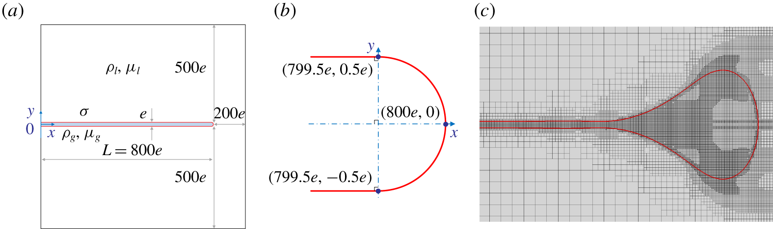
(a) Sketch of the computing domain. A long air sheet of thickness  $e$ and initial length
 $L=800e$ with a half-circle cap is extending horizontally at the centre of a square computing domain of liquid of size
 $1000e$. The sheet is connected to the left-hand boundary of the domain and has a free end
 $200e$ away from the right-hand boundary. The sheet thickness is not represented to scale for clarity. (b) Initial profile of the tip of the sheet. Two parallel lines are tangent lines to the half-circle at the connection point. (c) Snapshot of the adaptive mesh refinement in the area of the rim of the sheet for
 $Oh=0.3$ at
 $t^{\ast }=500$. The red curve represents the interface.

2 Problem and method
We consider a two-dimensional planar air sheet of uniform thickness  $e$ and initial length
 $L=800e$ in a square computing domain of size
 $1000e$ (figure 1). The sheet is set horizontally at an equal distance between the top and bottom boundaries. The air and the surrounding liquid are taken as incompressible. A symmetric boundary condition is imposed on the four sides of the domain, thus conserving the volume of air and liquid in the domain. The left-hand side of the air sheet reaches the side of the domain with a stable
 $90^{\circ }$ contact angle. The other side initially ends at
 $x=800e$ with a half-circular cap of diameter equal to the thickness
 $e$,
 $200e$ away from the right-hand boundary. The gas with density
 $\unicode[STIX]{x1D70C}_{g}$ and viscosity
 $\unicode[STIX]{x1D707}_{g}$ is surrounded by a liquid of density
 $\unicode[STIX]{x1D70C}_{l}$ and viscosity
 $\unicode[STIX]{x1D707}_{l}$, with surface tension
 $\unicode[STIX]{x1D70E}$. The air sheet contracts from rest under surface tension at a velocity
 $U$ and accumulates the displaced air into a rim. We verified that the initial shape of the rim and the size of the domain do not influence the contraction dynamics (see supplementary material, available at https://doi.org/10.1017/jfm.2020.385).
The dynamics are then characterised by the density ratio  $\unicode[STIX]{x1D6FC}=\unicode[STIX]{x1D70C}_{g}/\unicode[STIX]{x1D70C}_{l}$, the viscosity ratio
 $\unicode[STIX]{x1D6FD}=\unicode[STIX]{x1D707}_{g}/\unicode[STIX]{x1D707}_{l}$ and the Ohnesorge number
 $Oh$ that compares the viscous, capillary and inertial effects
 $$\begin{eqnarray}Oh=\frac{\unicode[STIX]{x1D707}_{l}}{\sqrt{\unicode[STIX]{x1D70C}_{l}\unicode[STIX]{x1D70E}e}}.\end{eqnarray}$$
The density and viscosity ratios are fixed to  $\unicode[STIX]{x1D6FC}=1.23\times 10^{-3}$ and
 $\unicode[STIX]{x1D6FD}=0.02$, and we vary systematically the Ohnesorge number
 $Oh$. The simulations parameters are chosen based on the properties of an air film contracting in water. For
 $Oh=0.1$, this would correspond to
 $e=1.1~\unicode[STIX]{x03BC}\text{m}$, which is consistent with the typical thickness of an air disk entrapped below an impacting drop (Thoroddsen et al. Reference Thoroddsen, Etoh and Takehara2003). Changing the
 $Oh$ would be equivalent physically to changing the film thickness
 $e$.
We solve the incompressible two-phase Navier–Stokes equations
 $$\begin{eqnarray}\displaystyle & \displaystyle \unicode[STIX]{x1D70C}\frac{D\boldsymbol{u}}{Dt}=-\unicode[STIX]{x1D735}p+\unicode[STIX]{x1D707}\unicode[STIX]{x0394}\boldsymbol{u}+\unicode[STIX]{x1D70E}\unicode[STIX]{x1D705}\unicode[STIX]{x1D6FF}_{s}\boldsymbol{n}, & \displaystyle\end{eqnarray}$$
 $$\begin{eqnarray}\displaystyle & \displaystyle \unicode[STIX]{x1D735}\boldsymbol{\cdot }\boldsymbol{u}=0, & \displaystyle\end{eqnarray}$$
where  $D/Dt$ denotes the material derivative,
 $p$ and
 $\boldsymbol{u}$ are the pressure and velocity,
 $\unicode[STIX]{x1D705}$ is the curvature of the interface,
 $\unicode[STIX]{x1D6FF}_{s}$ is a delta function to apply the surface tension at interface and
 $\boldsymbol{n}$ is the normal vector to the interface. The density
 $\unicode[STIX]{x1D70C}$ and viscosity
 $\unicode[STIX]{x1D707}$ take constant values in each phase.
The Navier–Stokes equations are solved in dimensionless form by the open source code Basilisk (Popinet Reference Popinet2019). We define the capillary-inertial velocity as  $U_{\unicode[STIX]{x1D70C}}=\sqrt{\unicode[STIX]{x1D70E}/(\unicode[STIX]{x1D70C}_{l}e)}$ and the capillary time as
 $\unicode[STIX]{x1D70F}_{\unicode[STIX]{x1D70C}}=\sqrt{\unicode[STIX]{x1D70C}_{l}e^{3}/\unicode[STIX]{x1D70E}}$. We then rescale the density, length, time, velocity and pressure by
 $\unicode[STIX]{x1D70C}_{l}$,
 $e$,
 $\unicode[STIX]{x1D70F}_{\unicode[STIX]{x1D70C}}$,
 $U_{\unicode[STIX]{x1D70C}}$ and
 $\unicode[STIX]{x1D70E}/e$, respectively. The non-dimensional equations can be written as
 $$\begin{eqnarray}\unicode[STIX]{x1D70C}^{\ast }\frac{D\boldsymbol{u}^{\ast }}{Dt^{\ast }}=-\unicode[STIX]{x1D735}^{\ast }p^{\ast }+Oh\unicode[STIX]{x1D707}^{\ast }\unicode[STIX]{x0394}\boldsymbol{u}^{\ast }+\unicode[STIX]{x1D705}^{\ast }\unicode[STIX]{x1D6FF}_{s}^{\ast }\boldsymbol{n},\end{eqnarray}$$
using an asterisk for dimensionless variables. The density  $\unicode[STIX]{x1D70C}^{\ast }$ and viscosity
 $\unicode[STIX]{x1D707}^{\ast }$ now take the value one in the liquid phase and
 $\unicode[STIX]{x1D6FC}$ and
 $\unicode[STIX]{x1D6FD}$ in the gas phase.
Basilisk uses a finite-volume method on an adaptive tree-structured (quad tree in two dimensions) mesh and the interface is tracked by a volume of fluid (VOF) method. Two criteria for mesh refinement were applied in our simulations based on the VOF tracer and the  $u$,
 $v$ components of the velocity. Figure 1(c) shows an example of the adaptive mesh refinement in the rim area, where the interface and regions of high vorticity are highly refined. The maximum level of refinement is characterised by the refinement level
 $n$ corresponding to a minimum cell size of
 $1/2^{n}$ times the size of the domain. The mesh independence was verified and
 $n=13$ was chosen in this study to guarantee at least eight meshes inside the air sheet thickness
 $e$, namely
 $2^{n}e/L\geqslant 8$ (see supplementary material). The simulation results were saved every
 $\unicode[STIX]{x0394}t^{\ast }=0.1$.
3 Dynamics of the air sheet contraction
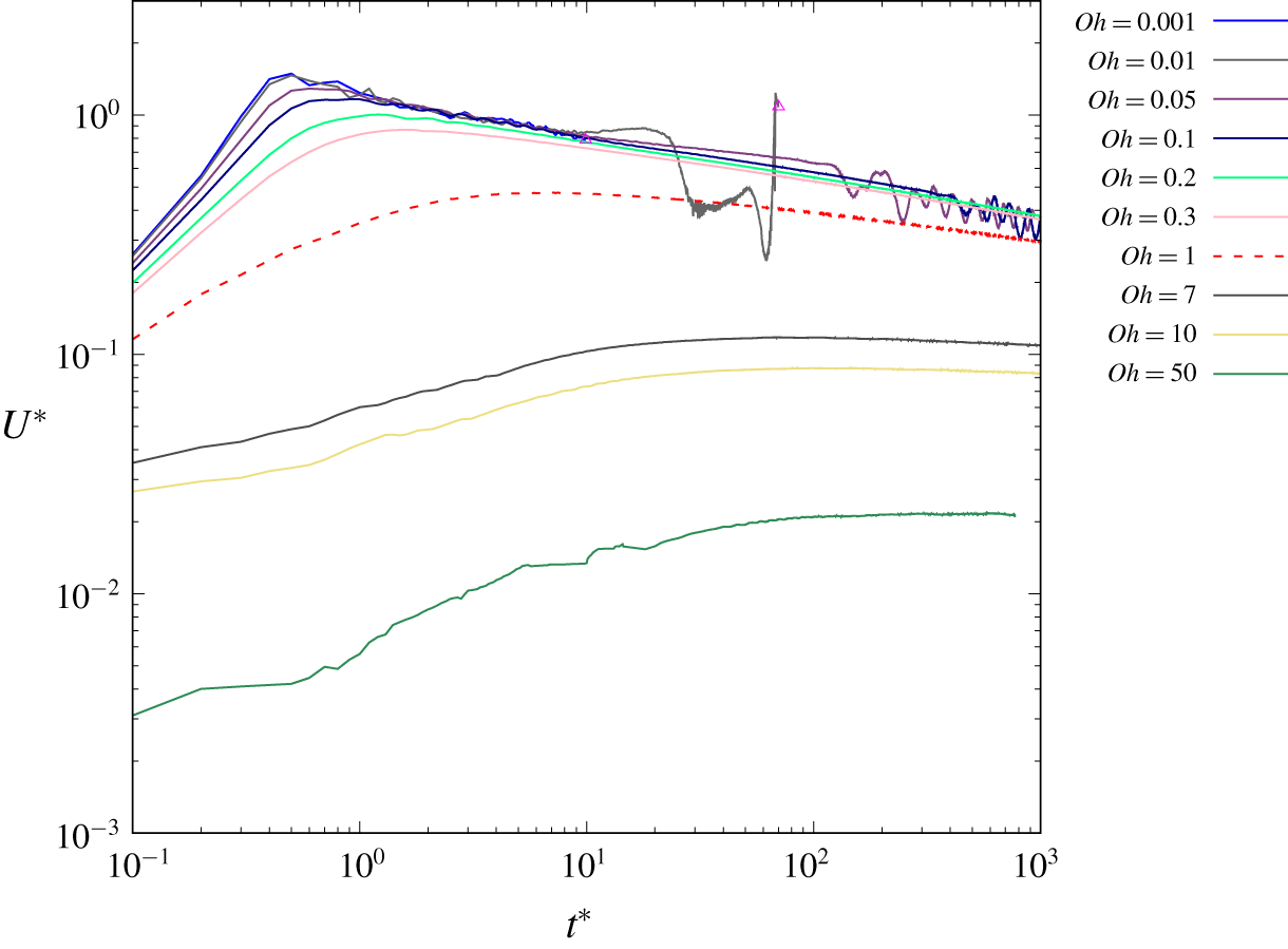
As the sheet starts contracting from rest under surface tension, the edge is accelerated and accumulates the gas into a rim (figure 1). The contraction velocity  $U^{\ast }$ increases to a maximum velocity
 $U_{max}^{\ast }$ before decreasing (figure 2), in a similar way as previously reported by Oguz & Prosperetti (Reference Oguz and Prosperetti1989) and Sob’yanin (Reference Sob’yanin2015). The contraction velocity increases more rapidly and to a higher
 $U_{max}^{\ast }$ for lower
 $Oh$. Some oscillations of the rim can be observed for
 $Oh\leqslant 0.1$ during the decreasing contraction velocity phase.
3.1 Maximum contraction velocity
Contraction velocity of the rim  $U^{\ast }=U/U_{\unicode[STIX]{x1D70C}}$ versus time
 $t^{\ast }=t/\unicode[STIX]{x1D70F}_{\unicode[STIX]{x1D70C}}$ for different Ohnesorge numbers
 $Oh$ in log–log scale. The data after pinch-off are not plotted, and the pinch-off time is indicated by an empty triangle at
 $t^{\ast }=10.0$ for
 $Oh=0.001$ and
 $t^{\ast }=72.5$ for
 $Oh=0.01$. A dashed line is used for
 $Oh=1$ to identify it more clearly (see supplementary material for the figure including the full range of
 $Oh$).

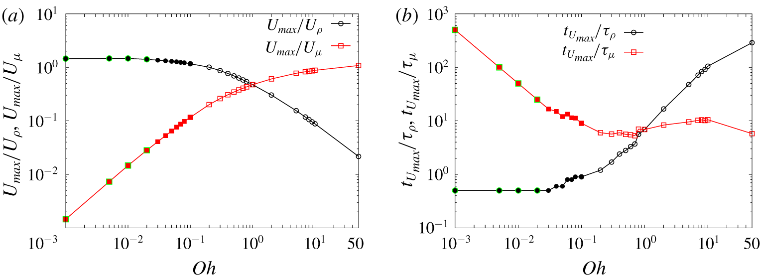
(a) Maximum contraction velocity of the rim  $U_{max}$ rescaled by the capillary-inertial velocity
 $U_{\unicode[STIX]{x1D70C}}=\sqrt{\unicode[STIX]{x1D70E}/(\unicode[STIX]{x1D70C}_{l}e)}$ and by the capillary-viscous velocity
 $U_{\unicode[STIX]{x1D707}}=\unicode[STIX]{x1D70E}/\unicode[STIX]{x1D707}_{l}$ as a function of the Ohnesorge number
 $Oh$ in log–log scale. (b) Time to reach the maximum velocity
 $t_{U_{max}}$ rescaled by the capillary-inertial time
 $\unicode[STIX]{x1D70F}_{\unicode[STIX]{x1D70C}}=\sqrt{\unicode[STIX]{x1D70C}_{l}e^{3}/\unicode[STIX]{x1D70E}}$ and by the capillary-viscous time
 $\unicode[STIX]{x1D70F}_{\unicode[STIX]{x1D707}}=\unicode[STIX]{x1D707}_{l}e/\unicode[STIX]{x1D70E}$, respectively, as a function of the Ohnesorge number
 $Oh$ in log–log scale. Solid symbols denote the cases for which the rim oscillates and solid symbols with green edges represent the cases with pinch-off. The dimensionless values used in the text are
 $U_{max}^{\ast }=U_{max}/U_{\unicode[STIX]{x1D70C}}$ and
 $t_{U_{max}}^{\ast }=t_{U_{max}}/\unicode[STIX]{x1D70F}_{\unicode[STIX]{x1D70C}}$.

As  $Oh$ tends to zero, the maximum contraction velocity converges to an asymptotic value
 $U_{max}^{\ast }=U_{max}/U_{\unicode[STIX]{x1D70C}}\simeq 1.5$ at
 $t_{U_{max}}^{\ast }=t_{U_{max}}/\unicode[STIX]{x1D70F}_{\unicode[STIX]{x1D70C}}=0.5$ before decreasing (figure 3). This scaling is characteristic of a capillary-inertial dominated dynamics. However, the maximum contraction velocity obtained here is larger than the Taylor–Culick velocity
 $U_{TC}^{\ast }=\sqrt{2}$ that would be obtained for a liquid film. Our results are consistent with the inviscid simulations of Oguz & Prosperetti (Reference Oguz and Prosperetti1989) focused on the initial contraction dynamics. They observed a maximum contraction velocity of approximately
 $U_{max-2D}^{\ast }\simeq 1.4$ for the two-dimensional simulations, larger than
 $U_{max-A}^{\ast }\simeq 1.2$ in the axisymmetric case. They even observed some oscillations of the contraction velocity during the acceleration phase, suggesting that the oscillations could appear even earlier in the inviscid limit. The antibubble rupture experiments of Dorbolo et al. (Reference Dorbolo, Caps and Vandewalle2003) and Zou et al. (Reference Zou, Ji, Yuan, Ruan and Fu2013) have a typical Ohnesorge number
 $Oh\simeq 0.1$, which is still in this capillary-inertial regime.
As the  $Oh$ number increases, the viscous dissipation decreases the maximum contraction velocity
 $U_{max}^{\ast }=U_{max}/U_{\unicode[STIX]{x1D70C}}$, and the time to reach this maximum
 $t_{U_{max}}^{\ast }=t_{U_{max}}/\unicode[STIX]{x1D70F}_{\unicode[STIX]{x1D70C}}$ increases towards infinity. If we rescale them by the capillary-viscous scales
 $U_{\unicode[STIX]{x1D707}}=\unicode[STIX]{x1D70E}/\unicode[STIX]{x1D707}_{l}$ and
 $\unicode[STIX]{x1D70F}_{\unicode[STIX]{x1D707}}=\unicode[STIX]{x1D707}_{l}e/\unicode[STIX]{x1D70E}$, the maximum contraction velocity
 $U_{max}/U_{\unicode[STIX]{x1D707}}$ converges towards an asymptotic value larger than one in a finite time
 $t_{U_{max}}/\unicode[STIX]{x1D70F}_{\unicode[STIX]{x1D707}}$ (figure 3), in a consistent way with the relations
 $$\begin{eqnarray}\displaystyle & \displaystyle \frac{U_{max}}{U_{\unicode[STIX]{x1D707}}}=Oh\,\frac{U_{max}}{U_{\unicode[STIX]{x1D70C}}}=Oh\,U_{max}^{\ast }, & \displaystyle\end{eqnarray}$$
 $$\begin{eqnarray}\displaystyle & \displaystyle \frac{t_{U_{max}}}{\unicode[STIX]{x1D70F}_{\unicode[STIX]{x1D707}}}=\frac{1}{Oh}\,\frac{t_{U_{max}}}{\unicode[STIX]{x1D70F}_{\unicode[STIX]{x1D70C}}}=\frac{1}{Oh}\,t_{U_{max}}^{\ast }. & \displaystyle\end{eqnarray}$$
This capillary-viscous scaling is similar to what was observed by Eggers et al. (Reference Eggers, Lister and Stone1999) and Reyssat & Quéré (Reference Reyssat and Quéré2006) for the contraction of an air film in a viscous liquid, or by Reyssat & Quéré (Reference Reyssat and Quéré2006) and Chebil et al. (Reference Chebil, McGraw, Salez, Sollogoub and Miquelard-Garnier2018) for the contraction of a liquid film in a viscous environment.
A similar trend to our figure 3(a) was also observed in Song & Tryggvason (Reference Song and Tryggvason1999) for the contraction of a liquid film. However, they underestimated the asymptotic contraction velocity due to a limited initial length of the film in their simulations (Sünderhauf et al. Reference Sünderhauf, Raszillier and Durst2002).
3.2 Three contraction regimes
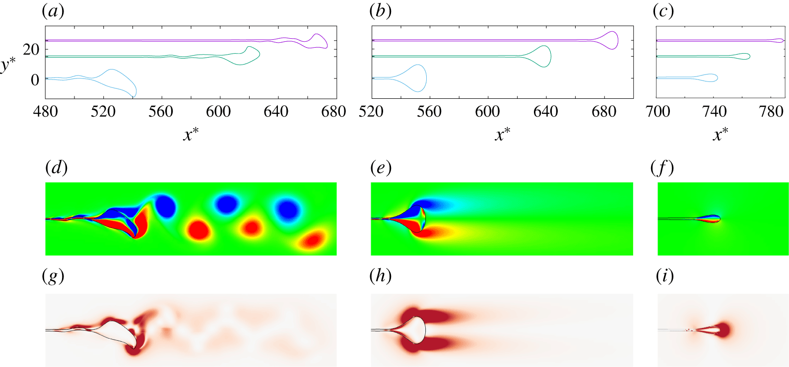
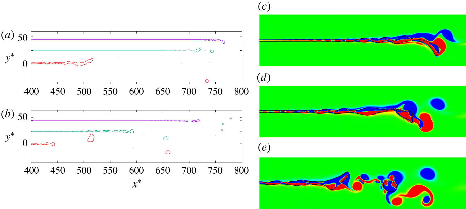
Three contraction dynamics regimes can be identified based on the Ohnesorge number  $Oh$, in a similar way as for the contraction of a liquid film (Brenner & Gueyffier Reference Brenner and Gueyffier1999; Savva & Bush Reference Savva and Bush2009): vortex shedding regime, smooth contraction regime and viscous regime (figure 4).
Three air film contraction regimes: (a,d,g,  $Oh=0.05$) vortex-shedding regime; (b,e,h,
 $Oh=0.3$) smooth-contraction; and (c,f,i,
 $Oh=7$) viscous regime. Panels (a–c) show the interface profile at
 $t^{\ast }=200,300,500$ from top to bottom, with equal unit length along
 $x^{\ast }=x/e$ and
 $y^{\ast }=y/e$ axis, with
 $t^{\ast }=t/\unicode[STIX]{x1D70F}_{\unicode[STIX]{x1D70C}}$. Panels (d–f) and panels (g–i) show snapshots of vorticity contour and viscous dissipation at
 $t^{\ast }=500$, respectively. The viscous dissipation rate is shown with a red shading in panels (g–i). See corresponding supplementary movies 1–3.

For  $Oh\leqslant 0.1$, some oscillations of the contraction velocity can be observed (figure 2). We formally define such oscillations when the
 $y$-coordinate of the
 $x$-maximum point of the air sheet is larger than half of the initial sheet thickness (
 $|y_{x_{max}}^{\ast }|>0.5$). These oscillations are characteristic of the deformations of the rim due to the shedding of vortices of alternating sign (figure 4a,d,g). This vorticity shedding is reminiscent of the von Kármán vortex street observed during the impact of a drop on a pool at high impact velocities (Thoraval et al. Reference Thoraval, Takehara, Etoh, Popinet, Ray, Josserand, Zaleski and Thoroddsen2012; Castrejón-Pita, Castrejón-Pita & Hutchings Reference Castrejón-Pita, Castrejón-Pita and Hutchings2012; Thoraval et al. Reference Thoraval, Takehara, Etoh and Thoroddsen2013). Capillary waves propagate from the rim to the bulk of the sheet, in a similar way as observed for the contraction of a liquid sheet at low
 $Oh$ numbers (Brenner & Gueyffier Reference Brenner and Gueyffier1999; Song & Tryggvason Reference Song and Tryggvason1999; Savva & Bush Reference Savva and Bush2009; Gordillo et al. Reference Gordillo, Agbaglah, Duchemin and Josserand2011). However, they do not remain symmetric across the centre of the sheet as for the liquid film, due to the vorticity shedding. The oscillations start earlier for smaller
 $Oh$ (figure 2). For low enough
 $Oh$ (
 $Oh\leqslant 0.02$), the oscillations can even induce the pinch-off of the rim (figure 5). The time of the first pinch-off decreases with decreasing
 $Oh$, at
 $t^{\ast }=862.5,72.5,13.0,10.0$ for
 $Oh=0.02,0.01,0.005,0.001$, respectively. The number of pinch-off events increases as the
 $Oh$ decreases, with only one pinch-off observed for
 $Oh=0.02$, and several pinch-offs for
 $Oh=0.01,0.005,0.001$. For the lowest
 $Oh$ numbers, the vorticity shedding becomes more irregular due to these pinch-off events (figure 5c–e). The rim oscillations are further analysed in § 4.4.
(a,b) Interface profiles of pinch-off: (a)  $Oh=0.01$ at
 $t^{\ast }=50,100,500$ from top to bottom; (b)
 $Oh=0.001$ at
 $t^{\ast }=100,300,500$ from top to bottom. The interface profiles are plotted with equal unit length along axis
 $x^{\ast }$ and
 $y^{\ast }$. The vertical position of the interface profile at
 $t^{\ast }=500$ corresponds to the vertical axis, while the other two profiles are translated up for clarity. (c–e) Snapshots of vorticity contour in the rim area for
 $Oh=0.01$ at
 $t^{\ast }=(c)~50$, (d) 72.5 and (e) 100, where pinch-off occurs at
 $t^{\ast }=72.5$ and the black curve represents the interface. Here,
 $x^{\ast }=x/e$,
 $y^{\ast }=y/e$ and
 $t^{\ast }=t/\unicode[STIX]{x1D70F}_{\unicode[STIX]{x1D70C}}$. See corresponding supplementary movie 4.

For larger  $Oh$ (
 $0.1<Oh\leqslant 1$), the contraction of the film enters the smooth contraction regime (figure 4b,e,h). The oscillations and capillary waves are damped by viscosity. The rim is more stable and rounded, with a pair of counter-rotating symmetric vortices attached to it without separation.
For even larger  $Oh$ (
 $Oh\gg 1$), the viscous effects are more pronounced, producing a more elongated rim in the longitudinal axis (figure 4c,f,i). Only limited vorticity is produced around the rim, with the rim slowly accelerating towards its maximum velocity. The shape of the rim is further characterised in § 4.1.
3.3 Asymptotic contraction velocity
For all  $Oh$ numbers, the rim velocity decreases after reaching the maximum contraction velocity. This decrease was attributed to a competition between surface tension force and a hydrodynamic drag force by Sob’yanin (Reference Sob’yanin2015) for the rupture of an antibubble. For low
 $Oh$ in our simulations, the decrease seems to follow a
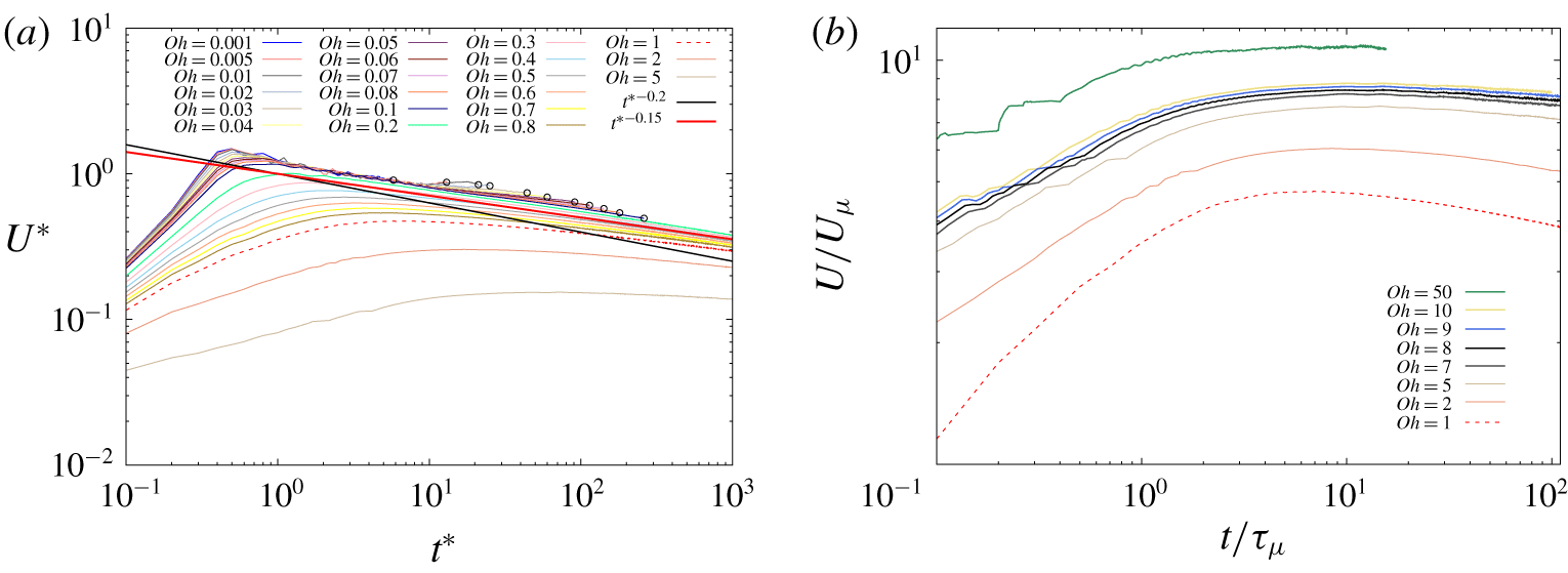
 $U\sim t^{-0.15}$ power law (figure 6a).
Contraction velocity of the rim versus time in log–log scale for (a)  $Oh\leqslant 5$ with comparison to the scaling law
 $U^{\ast }=t^{\ast -0.2}$ (black solid line) and
 $U^{\ast }=t^{\ast -0.15}$ (red solid line). The oscillations observed for
 $Oh\leqslant 0.1$ in figure 2 are not plotted. The starting time of the oscillations is formally defined as the time when the
 $y$-coordinate of the
 $x$-maximum point of the air sheet first overcomes the height of the sheet (
 $|y_{x_{max}}|>0.5e$), and indicated by an empty circle. A dashed line is used for
 $Oh=1$ for clarity. Here,
 $U^{\ast }=U/U_{\unicode[STIX]{x1D70C}}$,
 $t^{\ast }=t/\unicode[STIX]{x1D70F}_{\unicode[STIX]{x1D70C}}$. (b)
 $Oh\gg 1$: the velocity is rescaled by the capillary-viscous velocity
 $U_{\unicode[STIX]{x1D707}}=\unicode[STIX]{x1D70E}/\unicode[STIX]{x1D707}_{l}$ and time by the capillary-viscous time
 $\unicode[STIX]{x1D70F}_{\unicode[STIX]{x1D707}}=\unicode[STIX]{x1D707}_{l}e/\unicode[STIX]{x1D70E}$. Here,
 $Oh=1$, 2, 5 are included in both panels to capture the transition between the regimes.

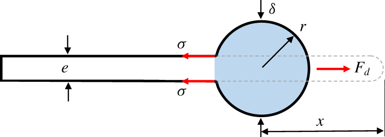
Sketch of force balance and mass conservation. The grey dashed line is the initial position of the air sheet and the blue area shows the accumulated mass at a later time  $t$. Here,
 $e$ is the initial thickness of the air sheet,
 $\unicode[STIX]{x1D6FF}$ is the thickness of the rim,
 $r$ is the radius of the rim assuming a circular shape,
 $x$ is the contraction distance,
 $\unicode[STIX]{x1D70E}$ is the surface tension force on the top and bottom interfaces of the air sheet and
 $F_{d}$ is the hydrodynamic drag force.

We can formulate a similar theory for the contraction of a two-dimensional air sheet as for the spherical geometry considered by Sob’yanin (Reference Sob’yanin2015). The surface tension force pulls on the rim from both the top and bottom interfaces (figure 7), leading to a total force on the rim  $F_{\unicode[STIX]{x1D70E}}$ (de Gennes et al. Reference de Gennes, Brochard-Wyart and Quéré2004),
 $$\begin{eqnarray}F_{\unicode[STIX]{x1D70E}}=2\unicode[STIX]{x1D70E}.\end{eqnarray}$$
It is balanced by the hydrodynamic drag force  $F_{d}$ on the rim of thickness
 $\unicode[STIX]{x1D6FF}$, which can be expressed as
 $$\begin{eqnarray}F_{d}={\textstyle \frac{1}{2}}\unicode[STIX]{x1D70C}_{l}U^{2}C_{d}\unicode[STIX]{x1D6FF}.\end{eqnarray}$$
The balance between the surface tension force  $F_{\unicode[STIX]{x1D70E}}$ and the hydrodynamic drag force
 $F_{d}$ gives
 $$\begin{eqnarray}2\unicode[STIX]{x1D70E}={\textstyle \frac{1}{2}}\unicode[STIX]{x1D70C}_{l}U^{2}C_{d}\unicode[STIX]{x1D6FF},\end{eqnarray}$$
leading to
 $$\begin{eqnarray}U=\sqrt{\frac{4\unicode[STIX]{x1D70E}}{\unicode[STIX]{x1D70C}_{l}C_{d}\unicode[STIX]{x1D6FF}}}.\end{eqnarray}$$
The contraction velocity of an air sheet therefore also follows a similar form as the Taylor–Culick velocity for the liquid film, but with a different length scale  $C_{d}\unicode[STIX]{x1D6FF}/2$ characteristic of the rim size rather than the film thickness.
If we assume that the rim is circular with radius  $r$,
 $\unicode[STIX]{x1D6FF}$ can be replaced by
 $2r$ in (3.6), leading to
 $$\begin{eqnarray}U=\sqrt{\frac{2\unicode[STIX]{x1D70E}}{\unicode[STIX]{x1D70C}_{l}C_{d}r}}.\end{eqnarray}$$
A second equation can be obtained from the conservation of mass of the air displaced. When the air sheet contracts to a distance  $x$ from the initial position, a volume of air
 $xe$ is then accumulated in the rim (figure 7),
 $$\begin{eqnarray}\unicode[STIX]{x03C0}r^{2}=xe.\end{eqnarray}$$
By substituting (3.8) into (3.7), we obtain the geometrical dependence of the contraction velocity  $U$,
 $$\begin{eqnarray}U=\left(\frac{\unicode[STIX]{x03C0}}{e}\right)^{0.25}\left(\frac{2\unicode[STIX]{x1D70E}}{\unicode[STIX]{x1D70C}_{l}C_{d}}\right)^{0.5}x^{-0.25}.\end{eqnarray}$$
Sob’yanin (Reference Sob’yanin2015) modelled the dynamics of the rim in the case of an antibubble rupture in the same way as a circular solid cylinder with a no-slip boundary condition and a constant drag coefficient  $C_{d}$. If we also assume a constant
 $C_{d}$, equation (3.9) can be solved analytically,
 $$\begin{eqnarray}U=\left(\frac{4\unicode[STIX]{x03C0}}{5e}\right)^{0.2}\left(\frac{2\unicode[STIX]{x1D70E}}{\unicode[STIX]{x1D70C}_{l}C_{d}}\right)^{0.4}t^{-0.2}.\end{eqnarray}$$
In dimensionless form this is
 $$\begin{eqnarray}U^{\ast }=Ct^{\ast -0.2},\quad \text{with }C=\left({\textstyle \frac{16}{5}}\unicode[STIX]{x03C0}\right)^{0.2}C_{d}^{-0.4}.\end{eqnarray}$$
This theory therefore predicts a power law decay of the contraction velocity in time. It is added as a black solid line in figure 6(a) with  $C=1$, corresponding to
 $C_{d}=3.17$. Although the trend is similar, we observe that the film contraction is consistently faster than this scaling, following a scaling closer to the red solid line in figure 6(a)
 $$\begin{eqnarray}U^{\ast }\sim t^{\ast -0.15}.\end{eqnarray}$$
This slightly different scaling of the contraction velocity decay could be due to several reasons.
(i) The theory of a constant drag coefficient established for solid cylinders with a no-slip surface does not apply here for an air cylinder. The boundary condition is closer to a free-slip boundary condition, due to the low density of the gas in the film. As argued by Legendre, Lauga & Magnaudet (Reference Legendre, Lauga and Magnaudet2009), the drag coefficient is reduced significantly by applying a shear-free boundary condition on a solid cylinder. A drag coefficient for bubbles can still be defined. However, experiments on the rising of a single bubble in water demonstrated that the drag coefficient
 $C_{d}$ shows fluctuation and $C_{d}$ is not only related to the Reynolds number but also to the geometry of the bubble (Tomiyama et al. Reference Tomiyama, Kataoka, Zun and Sakaguchi1998; Yan et al. Reference Yan, Jia, Wang and Cao2017). The variations of the drag coefficient could thus affect the scaling of the contraction velocity (see § 4.1).
(ii) We have assumed that the rim is circular to derive this power law decay. This is in sharp contrast with the Taylor–Culick velocity established for the contraction of a liquid film without any assumption on the shape of the rim. The air cylinder is not exactly a circle, with a shape evolving in time and with the
$Oh$ number (figure 4). The shape of the rim could also play a role in the scaling observed (see § 4.1).(iii) Finally, we have neglected the added mass of the surrounding liquid, characteristic of the accelerations of the rim. This will be important in the acceleration phase and in the oscillations regime, but can probably be neglected in the asymptotic regime as discussed by Sob’yanin (Reference Sob’yanin2015).


In the viscous regime at large  $Oh$, we expect the contraction velocity to reach the capillary-viscous velocity
 $U_{\unicode[STIX]{x1D707}}=\unicode[STIX]{x1D70E}/\unicode[STIX]{x1D707}_{l}$ over the time scale
 $\unicode[STIX]{x1D70F}_{\unicode[STIX]{x1D707}}=\unicode[STIX]{x1D707}_{l}e/\unicode[STIX]{x1D70E}$ and then decay slowly following a logarithmic correction (Reyssat & Quéré Reference Reyssat and Quéré2006). We have confirmed already these scalings for the maximum contraction velocity in figure 3. We focus here on the time evolution of the velocity after reaching the maximum (figure 6b). However, these high viscosity simulations require a longer computational time. The smaller decay regime observed in our simulations is not sufficient to obtain conclusive results about the asymptotic regime beyond the scaling velocity. Even if a 2-D asymptotic theory can be established, the two-dimensional assumption made in our simulations may not be physical, due to the three-dimensional destabilisation of the rim (Thoroddsen et al. Reference Thoroddsen, Thoraval, Takehara and Etoh2012). Further studies will therefore be needed to answer these questions.
3.4 Energy budget
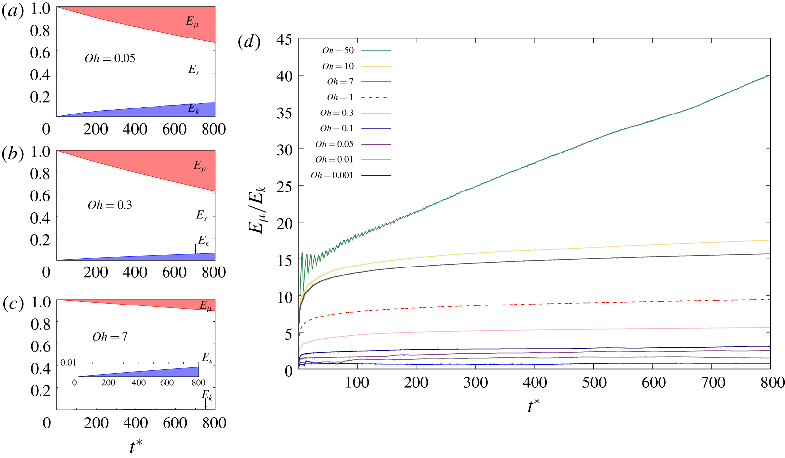
The drag coefficient model of the air film contraction presented above suggests that viscosity plays a more important role for the contraction of an air sheet compared to a liquid sheet. This is also suggested by the viscous dissipation around the vorticity regions observed in figure 4. The system initially only has surface energy  $E_{s0}$, converted to kinetic energy
 $E_{k}$ and viscous dissipation
 $E_{\unicode[STIX]{x1D707}}$ during the contraction (figure 8a–c). The rate of transfer is slower at higher
 $Oh$, due to the lower contraction velocity. However, a larger part is dissipated by viscous effects as the
 $Oh$ increases (figure 8d). This is in strong contrast to the contraction of a liquid sheet, for which the energy is equally distributed between the kinetic energy and viscous dissipation (Sünderhauf et al. Reference Sünderhauf, Raszillier and Durst2002; Savva & Bush Reference Savva and Bush2009). This behaviour is only observed at the lowest
 $Oh$ for the contraction of an air film, with
 $E_{\unicode[STIX]{x1D707}}/E_{k}\approx 1$ at
 $Oh=0.001$ (figure 8d). The fundamental difference between the contraction of an air film and a liquid film can therefore be explained by the stronger viscous dissipation effects for the air film.
(a–c) Temporal evolution of energy budget, with surface energy  $E_{s}$ in white, kinetic energy
 $E_{k}$ in blue and viscous dissipation
 $E_{\unicode[STIX]{x1D707}}$ in red, normalised by the initial surface energy
 $E_{s0}$ for the three regimes: (a) vortex-shedding regime,
 $Oh=0.05$, (b) smooth-contraction regime,
 $Oh=0.3$ and (c) viscous regime,
 $Oh=7$, corresponding to the three cases presented in figure 4. Inset in (c) is a zoom of the kinetic energy. (d) Ratio between viscous dissipation
 $E_{\unicode[STIX]{x1D707}}$ and kinetic energy
 $E_{k}$ versus time
 $t^{\ast }$. A dashed line is used for
 $Oh=1$ for clear view and
 $t^{\ast }=t/\unicode[STIX]{x1D70F}_{\unicode[STIX]{x1D70C}}$ (see supplementary material for the figure including the full range of
 $Oh$).

4 Dynamics of the rim
The first part of the analysis of the air sheet contraction dynamics was based on a dimensional analysis with the sheet thickness  $e$ as the relevant length scale. It provided a constant global Ohnesorge number
 $Oh=\unicode[STIX]{x1D707}_{l}/\sqrt{\unicode[STIX]{x1D70C}_{l}\unicode[STIX]{x1D70E}e}$ and constant velocity scales to characterise the dynamics of each simulation. However, the theoretical modelling of the contraction velocity derived in § 3.3 suggested that the contraction velocity of the rim is controlled by its thickness
 $\unicode[STIX]{x1D6FF}$ (see (3.6)). This implies that the contraction dynamics is better characterised by the time evolving local geometry of the rim rather than the thickness of the air sheet. This is also supported by the transitions to oscillations and pinch-off regimes of the rim triggered at earlier times for lower Ohnesorge numbers.
In this section, we therefore investigate the contraction dynamics of the air film considering the instantaneous geometry of the rim. We first analyse the rim geometry to verify the assumptions made for the modelling of the contraction velocity. We then focus on the triggering and dynamics of the rim oscillations. We discuss especially the relevance of the comparison with the flow around a solid cylinder, in terms of drag coefficient and transition to vortex shedding.
4.1 Rim geometry
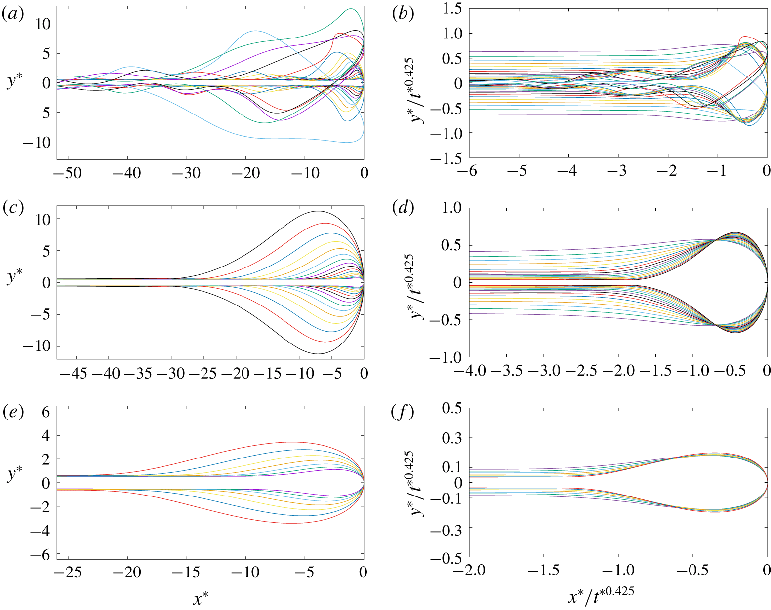
The evolution of the rim geometry with time and  $Oh$ is shown in figure 9(a,c,e), by translating horizontally the interface profiles to superpose the end points of the film. It confirms our modelling assumption that all the air displaced accumulates into a rim. The interface of the film beyond the rim is only disturbed at low
 $Oh$, first by capillary waves propagating from the rim, and then by asymmetric oscillations due to vortex shedding.
From the scaling law of the contraction velocity  $U^{\ast }\sim t^{\ast -0.15}$ observed at lower
 $Oh$ (3.12), the profiles of a circular rim would collapse together when rescaling both axis by
 $t^{\ast 0.425}$. The rescaled profiles presented in figure 9(b,d,f) indeed nearly overlap into a single shape, except for the oscillations regimes. However, we still observe some significant deviations, characteristic of the shape evolution of the rim, becoming more elongated in the vertical direction over time. The constant drag coefficient theory would have predicted a collapse of the rim profiles when rescaling by a slightly different power law
 $t^{\ast 0.4}$, from
 $U^{\ast }\sim t^{\ast -0.2}$ (3.11) as previously observed by Mirjalili, Chan & Mani (Reference Mirjalili, Chan and Mani2018). A similar collapse is also observed for this rescaling as presented in figure S9 of the supplementary material, due to the small difference of power law, but with significantly larger deviations.
Evolution of the rim profiles in the three regimes presented in figure 4: (a,b,  $Oh=0.05$) vortex-shedding regime, (c,d,
 $Oh=0.3$) smooth-contraction regime and (e,f,
 $Oh=7$) viscous regime. On the left-hand side (a,c,e), the profiles are translated to the same end point. On the right-hand side (b,d,f) both axis of the profiles are also rescaled by
 $t^{\ast 0.425}$. We show the first profile at the time of maximum contraction velocity
 $t_{1}^{\ast }=t_{U_{max}}^{\ast }$ to capture the stable regime of the contraction dynamics. Then the next time steps follow a logarithmic progression
 $t_{n+1}^{\ast }=1.5t_{n}^{\ast }$ to capture the slow evolution of the rim up to
 $t^{\ast }=1000$. The times of the first and last profiles are:
 $t_{1}^{\ast }=0.6$,
 $t_{19}^{\ast }=886.7$, at
 $Oh=0.05$;
 $t_{1}^{\ast }=1.7$,
 $t_{16}^{\ast }=744.4$, at
 $Oh=0.3$ and
 $t_{1}^{\ast }=71.4$,
 $t_{7}^{\ast }=813.3$, at
 $Oh=7$. Here,
 $x^{\ast }=x/e$,
 $y^{\ast }=y/e$ and
 $t^{\ast }=t/\unicode[STIX]{x1D70F}_{\unicode[STIX]{x1D70C}}$ (see supplementary material for the comparison between the rescaled profile deduced from the scaling law of contraction velocity
 $t^{\ast -0.15}$ and
 $t^{\ast -0.2}$).

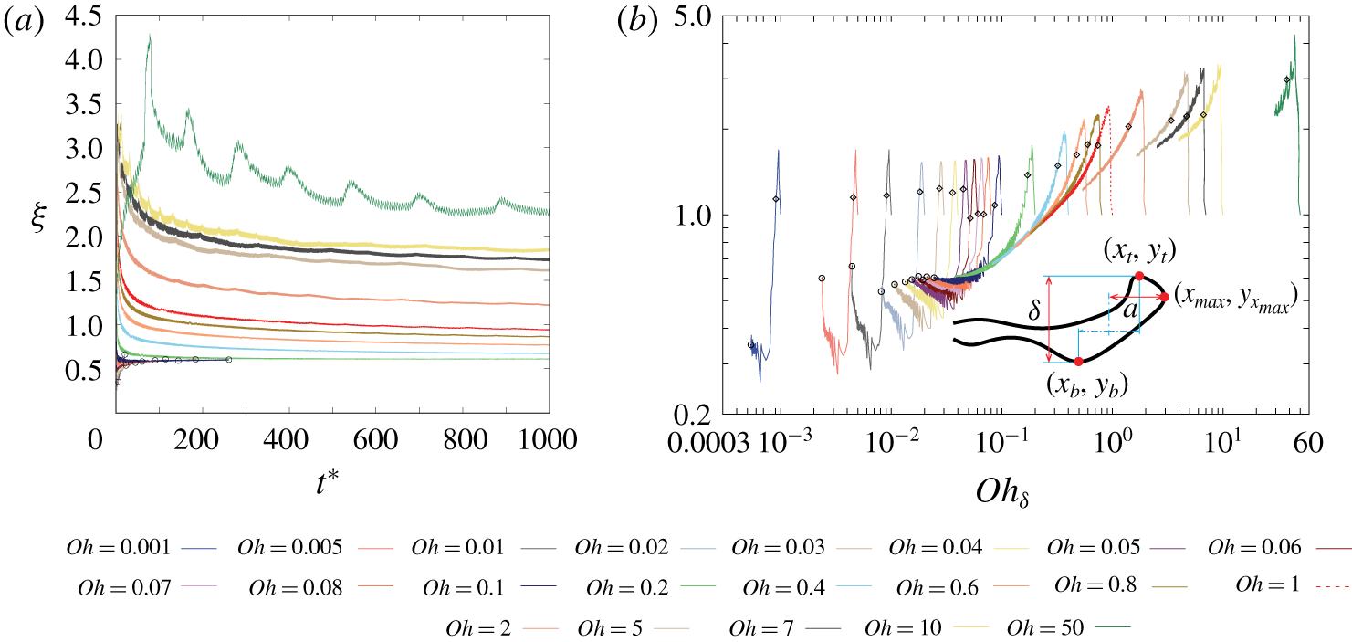
Aspect ratio of the rim  $\unicode[STIX]{x1D709}$ versus time
 $t^{\ast }$ in linear scale (a), and versus the local Ohnesorge number
 $Oh_{\unicode[STIX]{x1D6FF}}=\unicode[STIX]{x1D707}_{l}/\sqrt{\unicode[STIX]{x1D70C}_{l}\unicode[STIX]{x1D70E}\unicode[STIX]{x1D6FF}}$ in log–log scale (b). The aspect ratio
 $\unicode[STIX]{x1D709}$ corresponding to the maximum contraction velocity is indicated by an empty diamond, the aspect ratio
 $\unicode[STIX]{x1D709}$ corresponding to the starting time of the oscillations is indicated by an empty circle and the data after oscillation are not plotted for
 $Oh\leqslant 0.1$. Inset shows the definition of the aspect ratio
 $\unicode[STIX]{x1D709}=2a/\unicode[STIX]{x1D6FF}$ and the rim profile is taken from
 $Oh=0.05$ at
 $t^{\ast }=175$. A dashed line is used for
 $Oh=1$ for clarity. Here,
 $t^{\ast }=t/\unicode[STIX]{x1D70F}_{\unicode[STIX]{x1D70C}}$ (see supplementary material for the figure including the full range of
 $Oh$).

The deviations from a circular profile can be quantified by measuring the aspect ratio of the rim  $\unicode[STIX]{x1D709}$, defined as its horizontal size divided by its thickness (figure 10). It can be formally defined by tracking the dynamics of three characteristic points of the rim (see inset of figure 10b): the top point,
 $y$-maximum point
 $(x_{t},y_{t})$; the bottom point,
 $y$-minimum point
 $(x_{b},y_{b})$; and the end point,
 $x$-maximum point
 $(x_{max},y_{x_{max}})$. The aspect ratio of the rim
 $\unicode[STIX]{x1D709}$ is then defined as
 $\unicode[STIX]{x1D709}=2a/\unicode[STIX]{x1D6FF}$ with
 $a=x_{max}-0.5(x_{t}+x_{b})$ the horizontal distance between the
 $x$-maximum point of the rim
 $(x_{max},y_{x_{max}})$ and the centre of the rim
 $0.5(x_{t}+x_{b})$, and
 $\unicode[STIX]{x1D6FF}=y_{t}-y_{b}$ the thickness of the rim.
For all  $Oh$, the aspect ratio
 $\unicode[STIX]{x1D709}$ starts from the value one, corresponding to the half-circle initial profile of the edge. During the acceleration phase, it first increases rapidly, becoming more elongated horizontally, before decreasing. For the cases without oscillation (
 $Oh>0.1$), the aspect ratio then continues decreasing in time. This is consistent with the height of the rescaled rim increasing in time as observed in figure 9(d,f). As the
 $Oh$ increases, the aspect ratio curves move higher, corresponding to the flattening of the rim in the viscous regime observed in figure 9(e). In contrast, at low
 $Oh$ (
 $Oh\leqslant 0.1$) the decrease of the aspect ratio of the rim is much faster. After reaching a minimum value, corresponding to a maximal relative vertical extension, the aspect ratio
 $\unicode[STIX]{x1D709}$ then increases in time until oscillations. The oscillations of the rim then stretches it horizontally reaching values
 $\unicode[STIX]{x1D709}>1$ (see figure 9(a,b) and supplementary material).
The variations of  $\unicode[STIX]{x1D709}$ with time and
 $Oh$ can be understood from the local Ohnesorge number of the rim
 $Oh_{\unicode[STIX]{x1D6FF}}$, defined as
 $$\begin{eqnarray}Oh_{\unicode[STIX]{x1D6FF}}=\frac{\unicode[STIX]{x1D707}_{l}}{\sqrt{\unicode[STIX]{x1D70C}_{l}\unicode[STIX]{x1D70E}\unicode[STIX]{x1D6FF}}}.\end{eqnarray}$$
When plotted against  $Oh_{\unicode[STIX]{x1D6FF}}$ in figure 10(b), all the aspect ratios follow a similar trend, from a vertically elongated rim at low
 $Oh_{\unicode[STIX]{x1D6FF}}$ to a rim horizontally elongated at large
 $Oh_{\unicode[STIX]{x1D6FF}}$. The aspect ratio curves do not exactly collapse onto a single curve, suggesting that more parameters play a role in this correlation between the geometry and the local flow properties.
4.2 Drag coefficient
Drag coefficient  $C_{d}$, calculated as
 $C_{d}=4\unicode[STIX]{x1D70E}/(\unicode[STIX]{x1D70C}_{l}U^{2}\unicode[STIX]{x1D6FF})$ following (3.5), versus the local Reynolds number
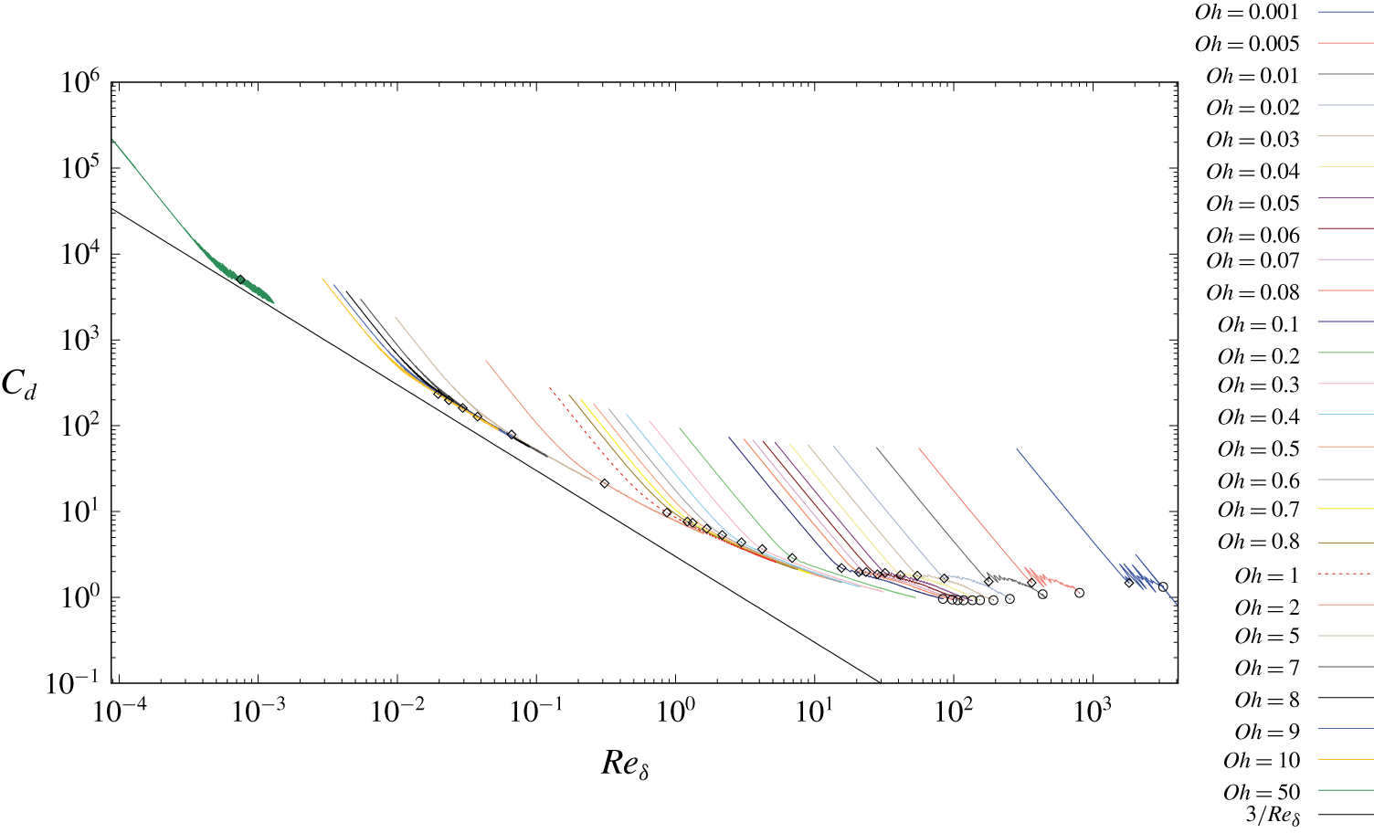
 $Re_{\unicode[STIX]{x1D6FF}}$ in log–log scale for different Ohnesorge numbers. The scaling
 $3/Re_{\unicode[STIX]{x1D6FF}}$ is plotted for comparison. The drag coefficient
 $C_{d}$ corresponding to the maximum contraction velocity is indicated by empty diamonds, the drag coefficient
 $C_{d}$ corresponding to the starting time of the oscillations is indicated by empty circles and the data after oscillation are not plotted for
 $Oh\leqslant 0.1$. A dashed line is used for
 $Oh=1$ to identify it more easily.

Based on this quantitative analysis of the rim geometry, we can discuss the validity of the modelling assumptions made in § 3.3. We can visualise the resistance of the flow to the motion of the rim by measuring the drag coefficient  $C_{d}$, estimated as
 $C_{d}=4\unicode[STIX]{x1D70E}/(\unicode[STIX]{x1D70C}_{l}U^{2}\unicode[STIX]{x1D6FF})$ from (3.5) only assuming a negligible added mass effect. In figure 11, we show
 $C_{d}$ as a function of the local Reynolds number
 $Re_{\unicode[STIX]{x1D6FF}}$ of the rim, defined as
 $$\begin{eqnarray}Re_{\unicode[STIX]{x1D6FF}}=\frac{\unicode[STIX]{x1D70C}_{l}U\unicode[STIX]{x1D6FF}}{\unicode[STIX]{x1D707}_{l}}.\end{eqnarray}$$
If we ignore the acceleration phase, affected by the added mass effect, a clear trend emerges, very similar to the drag coefficient of a solid cylinder. At low Reynolds numbers  $Re_{\unicode[STIX]{x1D6FF}}$,
 $C_{d}$ converges asymptotically towards a
 $Re_{\unicode[STIX]{x1D6FF}}^{-1}$ scaling, consistent with the capillary-viscous scaling of the contraction velocity
 $U_{\unicode[STIX]{x1D70E}}=\unicode[STIX]{x1D70E}/\unicode[STIX]{x1D707}_{l}$.
As the  $Re_{\unicode[STIX]{x1D6FF}}$ increases,
 $C_{d}$ deviates from that scaling and becomes more flat. The drag coefficients at the maximum contraction velocity (empty diamonds) converge towards an asymptotic value around 1.3. However,
 $C_{d}$ decreases systematically after this peak, and the
 $C_{d}$ does not collapse onto a master curve depending only on
 $Re_{\unicode[STIX]{x1D6FF}}$. This evolution of
 $C_{d}$ clearly illustrates the deviation of the contraction velocity from the constant drag coefficient theory
 $U^{\ast }=Ct^{\ast -0.2}$ discussed in § 3.3. If we consider the case of
 $Oh=0.1$, the aspect ratio is nearly constant before the oscillations as shown in figure 10(b). This deviation from the constant drag coefficient theory can therefore not be explained by this simple characterisation of the rim geometry. A more detailed analysis of the drag force around an air cylinder would be needed to better explain the scaling
 $U^{\ast }\sim t^{\ast -0.15}$ observed at low
 $Oh$. The curvature along the interface of the rim probably plays an important role, which cannot be captured by a simple aspect ratio measurement.
4.3 Transitions between the contraction regimes
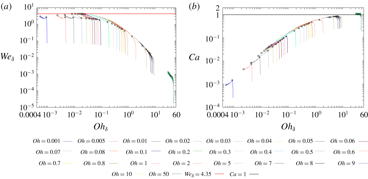
(a) Local Weber number  $We_{\unicode[STIX]{x1D6FF}}$, versus the local Ohnesorge number
 $Oh_{\unicode[STIX]{x1D6FF}}$ in log–log scale for different Ohnesorge numbers, and (b) capillary number
 $Ca$, versus the local Ohnesorge number
 $Oh_{\unicode[STIX]{x1D6FF}}$ in log–log scale for different Ohnesorge numbers. The constants
 $We_{\unicode[STIX]{x1D6FF}}=4.35$ and
 $Ca=1$ are plotted in panels (a) and (b), respectively, for comparison. The local Weber number
 $We_{\unicode[STIX]{x1D6FF}}$ and local capillary number
 $Ca$ corresponding to the maximum contraction velocity are indicated by empty diamond, the local Weber number
 $We_{\unicode[STIX]{x1D6FF}}$ and local capillary number
 $Ca$ corresponding to the starting time of the oscillations are indicated by empty circle and the data after oscillation are not plotted for
 $Oh\leqslant 0.1$. A dashed line is used for
 $Oh=1$ for clarity.

We observed that the contraction dynamics regime of an air sheet depends on the global Ohnesorge number  $Oh$, but also evolves in time with the local geometry of the rim. The relevant parameter to characterise the contraction dynamics of an air sheet is therefore its local Ohnesorge number
 $Oh_{\unicode[STIX]{x1D6FF}}$ based on the local time evolving thickness of the rim. At low local
 $Oh_{\unicode[STIX]{x1D6FF}}$, viscous effects can be neglected compared to inertia, and the dynamics can therefore be characterised by a local Weber number
 $We_{\unicode[STIX]{x1D6FF}}$,
 $$\begin{eqnarray}We_{\unicode[STIX]{x1D6FF}}=\frac{\unicode[STIX]{x1D70C}_{l}U^{2}\unicode[STIX]{x1D6FF}}{\unicode[STIX]{x1D70E}}.\end{eqnarray}$$
In contrast, at large  $Oh_{\unicode[STIX]{x1D6FF}}$ inertia can be neglected compared to viscous effects, leading to the dynamics controlled by a local capillary number
 $Ca$,
 $$\begin{eqnarray}Ca=\frac{\unicode[STIX]{x1D707}_{l}U}{\unicode[STIX]{x1D70E}}.\end{eqnarray}$$
This transition between the two asymptotic regimes during the contraction is clearly illustrated in figure 12, showing the time evolution of the local  $We_{\unicode[STIX]{x1D6FF}}$ and
 $Ca$ as a function of the
 $Oh_{\unicode[STIX]{x1D6FF}}$. It corresponds to the local equivalent of figure 3(b) including the complete time evolution of the contraction dynamics.
The local Weber number  $We_{\unicode[STIX]{x1D6FF}}$ corresponds to the square of the contraction velocity non-dimensionalised by a capillary-inertial velocity based on the local rim thickness
 $\unicode[STIX]{x1D6FF}$ rather than the film thickness
 $e$, as presented in figure 2. According to the theory presented in § 3.3,
 $We_{\unicode[STIX]{x1D6FF}}$ should be constant in the capillary-inertial regime (see (3.6)). This corresponds also to the constant drag coefficient at large
 $Re_{\unicode[STIX]{x1D6FF}}$ discussed previously, considering that
 $We_{\unicode[STIX]{x1D6FF}}=4/C_{d}$ with the definition used in figure 11. However, the
 $We_{\unicode[STIX]{x1D6FF}}$ still evolves in time for all air film contractions in the low viscosity regime. This time evolution in the smooth contraction regime reaches a consistent maximum of
 $We_{\unicode[STIX]{x1D6FF}}=4.35$ when the rim starts oscillating (see figure 12a). This critical local Weber number
 $We_{\unicode[STIX]{x1D6FF}}$ therefore characterises the transition to the oscillations of the rim. The critical
 $Re_{\unicode[STIX]{x1D6FF}}$ leading to the oscillations thus increases with decreasing
 $Oh_{\unicode[STIX]{x1D6FF}}$, in contrast with the flow around a solid cylinder where the vortex shedding appears at a characteristic Reynolds number.
In contrast, at large  $Oh_{\unicode[STIX]{x1D6FF}}$ the capillary number
 $Ca$ converges towards an asymptotic value around
 $Ca=1$ (see figure 12b). This local characterisation of the rim dynamics better illustrates this capillary viscous limit than the time evolution curves presented in figure 6, showing that the rim evolves towards lower values of
 $Oh_{\unicode[STIX]{x1D6FF}}$ in time.
4.4 Oscillations of the rim
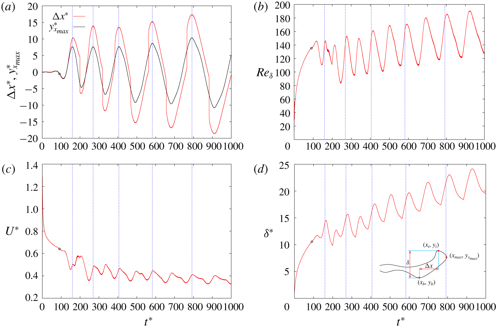
We observed earlier that in the low Ohnesorge regime  $Oh\leqslant 0.1$, some oscillations appear on the contraction velocity (figure 2), characteristic of the rim oscillations and vorticity shedding (figure 4a,d,g). These oscillations are qualitatively similar to the vortex induced oscillations of a flexible cylinder (Williamson & Govardhan Reference Williamson and Govardhan2004). In this section, we analyse these oscillations, and their influence on the contraction velocity. As defined in § 3.2, we formally define such oscillations as when the
 $y$-coordinate of the
 $x$-maximum point of the air sheet is larger than half of the initial sheet thickness (
 $|y_{x_{max}}^{\ast }|>0.5$).
Time evolution of the oscillation of the rim at  $Oh=0.05$. (a) Difference of
 $x$-coordinates between the top and bottom points of the rim
 $\unicode[STIX]{x0394}x^{\ast }$ versus time
 $t^{\ast }$ and
 $y$-coordinate of the
 $x$-maximum point of the rim
 $y_{x_{max}}^{\ast }$ versus time
 $t^{\ast }$. (b) Local Reynolds number of the rim
 $Re_{\unicode[STIX]{x1D6FF}}$ versus time
 $t^{\ast }$. (c) Contraction velocity of the rim
 $U^{\ast }$ versus time
 $t^{\ast }$. (d) Thickness of the rim
 $\unicode[STIX]{x1D6FF}^{\ast }$ versus time
 $t^{\ast }$, inset shows the definition of
 $\unicode[STIX]{x0394}x^{\ast }=x_{t}^{\ast }-x_{b}^{\ast }$ and
 $\unicode[STIX]{x1D6FF}^{\ast }=y_{t}^{\ast }-y_{b}^{\ast }$, the rim profile is taken from
 $Oh=0.05$ at
 $t^{\ast }=175$. Vertical dashed lines indicate the reference time used to measure the oscillations period. The starting time of the oscillations is indicated by an empty circle. Here,
 $x^{\ast }=x/e$,
 $y^{\ast }=y/e$,
 $U^{\ast }=U/U_{\unicode[STIX]{x1D70C}}$ and
 $t^{\ast }=t/\unicode[STIX]{x1D70F}_{\unicode[STIX]{x1D70C}}$.

We track the three characteristic points of the rim defined in § 4.1 (also see inset of figure 13d): the top point,  $y$-maximum point
 $(x_{t},y_{t})$; the bottom point,
 $y$-minimum point
 $(x_{b},y_{b})$; and the end point,
 $x$-maximum point
 $(x_{max},y_{x_{max}})$. The time evolution of the rim geometry can be derived from these points, with a typical example shown in figure 13 for
 $Oh=0.05$. We observe that the smooth oscillations of the rim geometry are well correlated with the oscillations of the contraction velocity. The difference of
 $x$-coordinates between the top and bottom point of the rim (
 $\unicode[STIX]{x0394}x^{\ast }=x_{t}^{\ast }-x_{b}^{\ast }$), and the
 $y$-coordinate of the
 $x$-maximum point of the rim
 $y_{x_{max}}^{\ast }$ both oscillate and show good consistence in periodicity. The contraction velocity
 $U^{\ast }$ oscillates with a decreasing average
 $\overline{U^{\ast }}$ in time (figure 13c), calculated over one oscillation period. The thickness of the rim (
 $\unicode[STIX]{x1D6FF}^{\ast }=y_{t}^{\ast }-y_{b}^{\ast }$) oscillates with an increasing average
 $\overline{\unicode[STIX]{x1D6FF}^{\ast }}$ (figure 13d). As a result, the local Reynolds number
 $Re_{\unicode[STIX]{x1D6FF}}$ oscillates with an increasing average
 $\overline{Re_{\unicode[STIX]{x1D6FF}}}$ during the contraction (figure 13b).
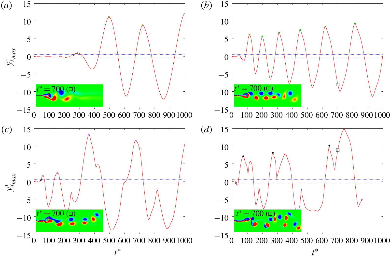
The  $y$-coordinate of the
 $x$-maximum point of the rim
 $y_{x_{max}}^{\ast }$ versus time
 $t^{\ast }$ at (a)
 $Oh=0.1$, (b)
 $Oh=0.04$, (c)
 $Oh=0.03$ and (d)
 $Oh=0.02$. Insets show the vorticity contour at
 $t^{\ast }=700$ (indicated by an empty square on the curve). Horizontal dashed lines indicate the threshold of oscillation
 $y^{\ast }=0.5$ and
 $y^{\ast }=-0.5$. Filled circles indicate the boundaries of a period used to calculate the average Strouhal number
 $\overline{St}$ and different colour is used for different Ohnesorge number as in figure 15. The starting time of the oscillations is indicated by an empty circle. The data after pinch-off are not plotted for
 $Oh=0.02$, with the pinch-off time indicated by an empty triangle at
 $t^{\ast }=862.5$. Here,
 $y^{\ast }=y/e$ and
 $t^{\ast }=t/\unicode[STIX]{x1D70F}_{\unicode[STIX]{x1D70C}}$ (see supplementary material for additional figures with Ohnesorge numbers from
 $Oh=0.02$ to
 $Oh=0.2$).

For  $0.04\leqslant Oh\leqslant 0.1$, the oscillations of
 $y_{x_{max}}^{\ast }$ are quite regular (see figure 13, figure 14 and the supplementary material for the other curves). The period and amplitude of these oscillations both increase in time, as indicated by the vertical dashed lines in figure 13. These oscillations are consistent with the shedding of alternating sign vortices, forming a vortex street as observed in the insets of figure 14. The oscillations start earlier and with a higher frequency for lower
 $Oh$.
As the  $Oh$ further decreases, the oscillations become more irregular. For
 $Oh=0.03$, some higher amplitude oscillations develop with a longer period, modulated by a smaller amplitude oscillation. For
 $Oh=0.02$, the
 $y_{x_{max}}^{\ast }$ profile shows a ‘double peaks’ shape in a half-period of oscillation, each peak corresponding to a vortex shedding event. The rim eventually detaches from the sheet at
 $t^{\ast }=862.5$. For
 $Oh\leqslant 0.01$, the fast deformations of the interface lead to pinch-off rapidly during the contraction, which does not show regular oscillations anymore.
We can quantify the variations of the oscillations frequency  $f=1/T$ by defining the Strouhal number as
 $$\begin{eqnarray}St=\frac{f\unicode[STIX]{x1D6FF}}{U},\end{eqnarray}$$
where  $\unicode[STIX]{x1D6FF}$ is the rim thickness and
 $U$ the contraction velocity. We estimate the oscillation period
 $T$ by taking the time difference between each positive peak of
 $y_{x_{max}}^{\ast }$, indicated as filled circles in figure 14. Only the large amplitude oscillations across the centre line of the film are considered by taking only the first positive peak of
 $y_{x_{max}}^{\ast }$. Since the thickness of the rim and the contraction velocity oscillate in time, we take the average value of
 $\unicode[STIX]{x1D6FF}/U$ in a period
 $T$ to calculate an average Strouhal number
 $\overline{St}$.
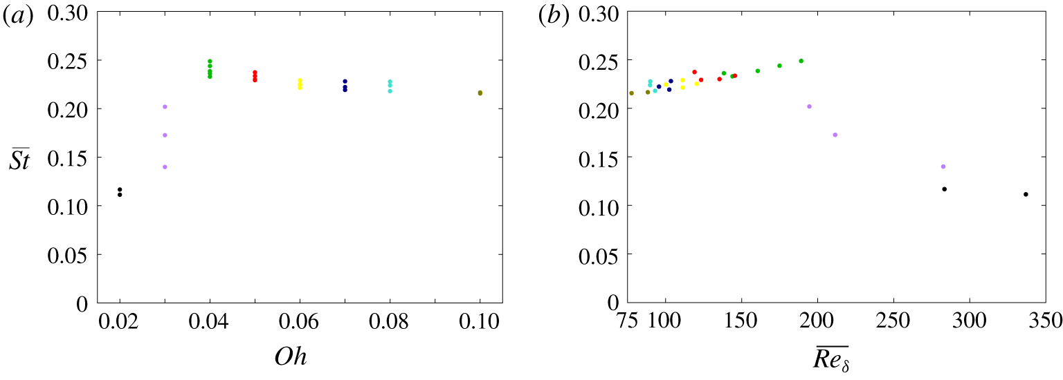
As shown in figure 15(a), the average Strouhal number  $\overline{St}$ of these oscillations stays between 0.22 and 0.25 when
 $0.04\leqslant Oh\leqslant 0.1$, with a slight decrease with
 $Oh$. Lower values of
 $\overline{St}$ are observed for
 $Oh=0.03$ and
 $Oh=0.02$, characteristic of the multiple vorticity shedding events over a longer period of oscillation. The evolution of the
 $\overline{St}$ can be understood from the local properties of the flow around the rim, in a similar way as for the vorticity shedding behind a solid cylinder. A consistent behaviour emerges if we plot
 $\overline{St}$ as a function of the average local Reynolds number
 $\overline{Re_{\unicode[STIX]{x1D6FF}}}$ over the oscillation period in figure 15(b). For
 $\overline{Re_{\unicode[STIX]{x1D6FF}}}<200$,
 $\overline{St}$ increases slightly with
 $\overline{Re_{\unicode[STIX]{x1D6FF}}}$, from 0.22 to 0.25. A clear transition is observed at
 $\overline{Re_{\unicode[STIX]{x1D6FF}}}\approx 200$. For
 $\overline{Re_{\unicode[STIX]{x1D6FF}}}>200$, the average Strouhal number
 $\overline{St}$ decreases with
 $\overline{Re_{\unicode[STIX]{x1D6FF}}}$, corresponding to a more complex vorticity shedding.
Average Strouhal number  $\overline{St}$ versus Ohnesorge number
 $Oh$ (a) and versus the average local Reynolds number
 $\overline{Re_{\unicode[STIX]{x1D6FF}}}$ (b) for
 $0.02\leqslant Oh\leqslant 0.1$. Different colours are used for the different Ohnesorge numbers.

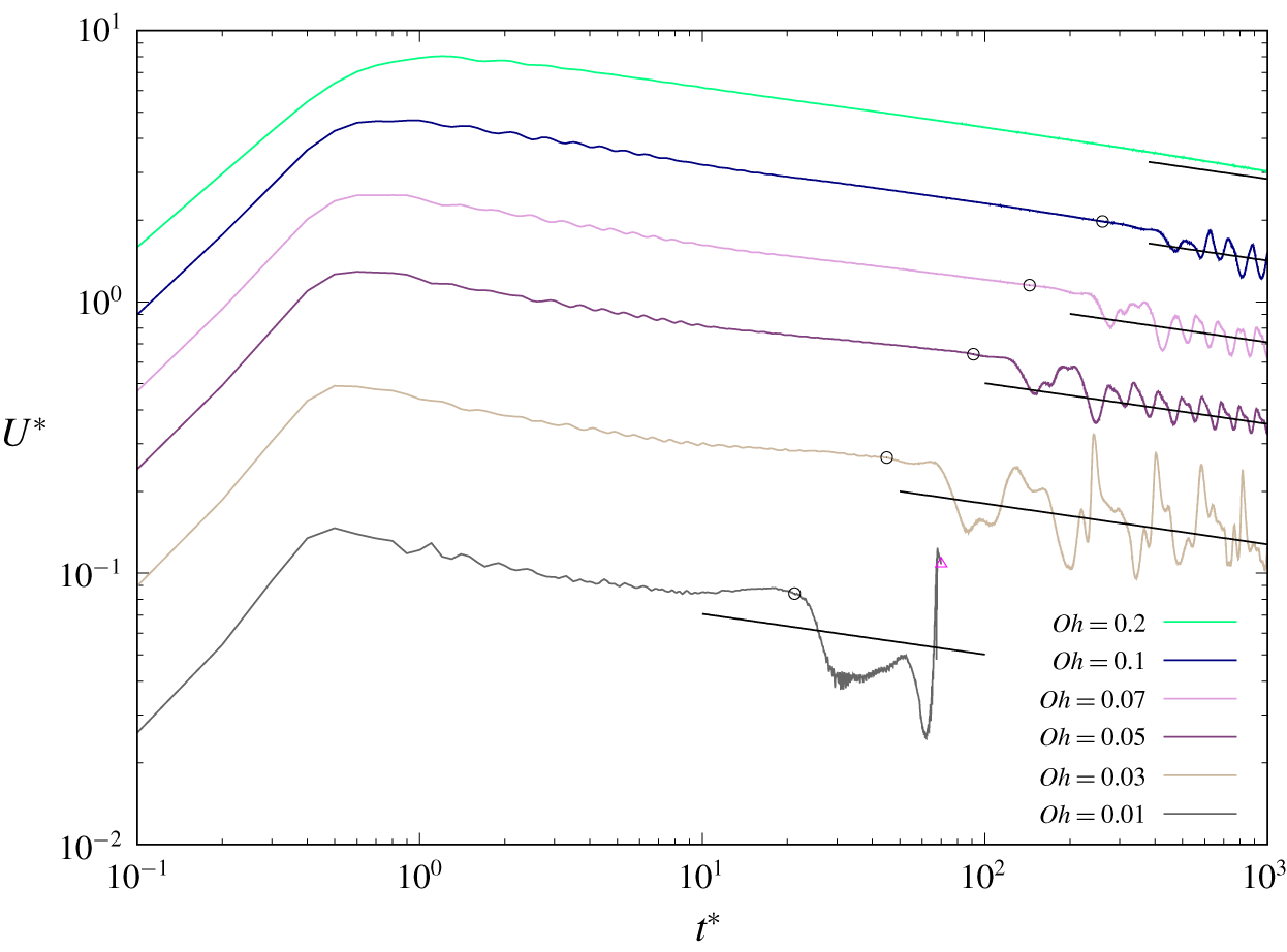
Average contraction velocity of the oscillation regime for different Ohnesorge numbers in log–log scale. The vertical position of the curve for  $Oh=0.05$ corresponds to the vertical axis values and the other curves are shifted vertically for clear view. The same scaling law of the contraction velocity
 $U^{\ast }=t^{\ast -0.15}$ (black line) is plotted in the oscillation part for all the Ohnesorge numbers. The starting time of the oscillations is indicated by an empty circle. The data after pinch-off are not plotted for
 $Oh=0.01$, with the pinch-off time indicated by an empty triangle at
 $t^{\ast }=72.5$. The non-oscillating case
 $Oh=0.2$ is plotted for comparison. Here,
 $U^{\ast }=U/U_{\unicode[STIX]{x1D70C}}$ and
 $t^{\ast }=t/\unicode[STIX]{x1D70F}_{\unicode[STIX]{x1D70C}}$.

The influence of these oscillations on the contraction velocity is shown in figure 16. As expected, the mean contraction velocity decreases when the rim enters into the oscillations regime, due to the increased added mass and viscous dissipation. However, it still follows the same scaling  $U^{\ast }\sim t^{\ast -0.15}$ on average.
5 Conclusion
We have investigated the contraction of a two-dimensional air sheet in a surrounding liquid by solving the two-dimensional two-phase Navier–Stokes equations. We have confirmed that in a large range of Ohnesorge numbers, the contraction dynamics follow a similar trend, with an initial increase to a maximum velocity before decreasing. The maximum contraction velocity converges towards a capillary-inertial velocity at low  $Oh$ and a capillary-viscous velocity at high
 $Oh$. We have identified three different regimes of the contraction dynamics, in a similar way as for the contraction of a liquid film. At low
 $Oh$ (
 $Oh\leqslant 0.1$), the contracting rim sheds vortices of alternating signs and some capillary waves propagate ahead of the rim. The deformations induced can eventually lead to the pinch-off of bubbles at the lowest
 $Oh$ (
 $Oh\leqslant 0.02$). At intermediate
 $Oh$ (
 $0.1<Oh\leqslant 1$), the contraction of a rounded rim is stabilised by viscosity. At larger
 $Oh$, the rim becomes more elongated with a viscosity limited contraction velocity.
We found that the asymptotic contraction velocity follows a scaling  $U\sim t^{-0.15}$ that is different from the scaling
 $t^{-0.2}$ deduced under the assumption of a constant drag coefficient. We explained the fundamental differences between the contraction of a liquid film and an air film by the increased ratio of energy dissipated by viscous effects.
The dynamics of an air sheet can be understood by the local properties of the flow. The transition between the capillary-viscous and capillary-inertial regimes is a time evolving process characterised by the local Ohnesorge number  $Oh_{\unicode[STIX]{x1D6FF}}$. The analogy with a solid cylinder shows similar scalings of the drag coefficient and oscillation frequency. However, the transition to oscillations is characterised for the contraction of an air sheet by a critical local Weber number
 $We_{\unicode[STIX]{x1D6FF}}$.
An air sheet contracting in a surrounding liquid will eventually break up due to three-dimensional instabilities (Thoroddsen et al. Reference Thoroddsen, Thoraval, Takehara and Etoh2012) relevant for the formation of microbubbles in turbulent breaking waves (Chan et al. Reference Chan, Mirjalili, Jain, Urzay, Mani and Moin2018, Reference Chan, Mirjalili, Jain, Urzay, Mani and Moin2019). Further three-dimensional simulations and modelling are therefore needed to understand these instabilities and investigate their effect on the dynamics of the rupturing front. It will be interesting, especially, to understand if the vorticity shedding and vertical oscillations predicted in 2-D simulations at low  $Oh$ can be observed experimentally, as for the vortex street observed below an impacting drop (Castrejón-Pita et al. Reference Castrejón-Pita, Castrejón-Pita and Hutchings2012; Thoraval et al. Reference Thoraval, Takehara, Etoh, Popinet, Ray, Josserand, Zaleski and Thoroddsen2012, Reference Thoraval, Takehara, Etoh and Thoroddsen2013), or if the 3-D instabilities prevent their coherent formation. These oscillations could provide a theoretical 2-D path to the rupture of air films, but may never be observed experimentally due to 3-D effects.
Acknowledgements
Z.J. acknowledges the financial support from the National Natural Science Foundation of China (grant no. 11802226). P.D. and M.-J.T. acknowledge the helpful discussions with A. Berny and T. Séon. M.-J.T. acknowledges the financial support from the National Natural Science Foundation of China (grant nos. 11542016, 11702210 and 11850410439) and the Project B18040. M.-J.T. is also supported by the Cyrus Tang Foundation through the Tang Scholar program.
Declaration of interests
The authors report no conflict of interest.
Supplementary material and movies
Supplementary material and movies are available at https://doi.org/10.1017/jfm.2020.385.