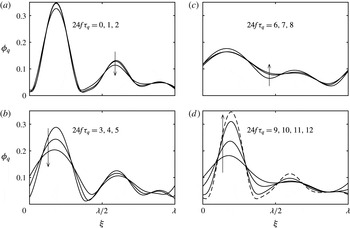
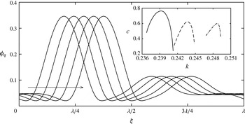
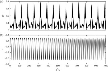
1 Introduction
On the free surfaces of viscous fluids, thermal gradients translate to surface stresses that drive bulk phase motion. Known either as the Marangoni effect, or thermocapillarity, the phenomenon describes the dynamic motions that arise from the temperature dependence of surface tension. Whereas in many cases the temperature gradients are used to effect an outcome, such as droplet migration, climbing films and convection in closed cavities, it also plays a crucial role in applications such as crystal growth stabilization and heat transfer operations.
Among the earliest experiments on thermocapillarity were carried out by Bénard (Reference Bénard1900), who investigated convection cells generated by heating a fluid layer from below. Pearson (Reference Pearson1958) clarified that thermocapillary stresses were of greater significance at the experimental layer heights, even though buoyancy can drive convection in this set-up. This instability is now referred to as the Pearson mode, and is characterized by a short (finite) wavelength and negligible surface deformation. For smaller layer heights, Scriven & Sternling (Reference Scriven and Sternling1964) suggested that a long-wavelength, deformational mode becomes dominant. The competition between the short- and long-wavelength modes was clearly highlighted by the experiments of VanHook et al. (Reference VanHook, Schatz, Swift, McCormick and Swinney1997). They also observed that the long-wavelength mode grows until rupture, in accordance with their theoretical prediction that bifurcation is subcritical.
These fundamental works on thermocapillarity have considered fluids whose surface tension is approximated as a linearly decreasing function of temperature. Hence, surface tractions act to drag fluid away from locations on a free surface that are locally hot. We refer to this behaviour as ‘linear surface tension’. Exceptions to this rule that motivate our work are dilute aqueous long-chain alcohols. The surface tensions of these mixtures exhibit well-defined minima at specific temperatures, see Vochten & Pétré (Reference Vochten and Pétré1973), Ono et al. (Reference Ono, Kaneko, Nishiguchi and Shoji2009), and usually are modelled as quadratic functions of temperature. Due to their unique behaviour in boiling processes, Abe (Reference Abe2006) labelled these fluids as ‘self-rewetting’. Anomalous thermocapillary effects using self-rewetting fluids have been investigated for migration of bubbles by Shanahan & Sefiane (Reference Shanahan and Sefiane2014) and Tripathi et al. (Reference Tripathi, Sahu, Karapetsas, Sefiane and Matar2015) and droplets by Karapetsas et al. (Reference Karapetsas, Sahu, Sefiane and Matar2014).
The most dramatic applications of self-rewetting fluids were first anticipated by Zhang (Reference Zhang2001), who suggested they could be used to enhance heat pipe performance. He noted that, in boiling situations, thermocapillary stresses would direct flow towards nucleation sites, thereby counteracting film dry out. Following his suggestion, experimental works have somewhat unanimously reported that self-rewetting fluids enhance heat transfer, for several different heat pipe configurations, including: Fracescantonio, Savino & Abe (Reference Fracescantonio, Savino and Abe2008), Savino et al. (Reference Savino, Paola, Cecere and Fortezza2010), Hu et al. (Reference Hu, Liu, Li and Wang2014) and Wu (Reference Wu2015). Some experiments have investigated films of self-rewetting fluids. In a pulsating heat pipe of diameter 1.8 mm, Fumoto et al. (Reference Fumoto, Ishida, Kawanami and Inamura2015) observed surface waves on aqueous butanol and pentanol films that enclose vapour plugs. Sitar & Golobic (Reference Sitar and Golobic2015) have characterized the role of self-rewetting films on heat transfer at even smaller scales. In their experiment, aqueous butanol was continuously pumped through
 $25\times 25$
or
 $50\times 50~\unicode[STIX]{x03BC}$
m square channels, which were heated so that a time-periodic boiling flow results. During the boiling period, when the apparent channel contact line recedes, an annular film is deposited that grows to approximately 1 mm in length, at which point the channel starts to refill. Anomalous surface tension clearly stabilizes this film and enhances heat transfer relative to water flows through their device, which do not deposit films.
It is generally accepted that heat and mass transfer of processes utilizing falling films are enhanced by conditions that generate wavy, non-rupturing films. See, for example, Goren & Mani (Reference Goren and Mani1968), Kalliadasis et al. (Reference Kalliadasis, Ruyer-Quil, Scheid and Velarde2012) and Frisk & Davis (Reference Frisk and Davis2015). Because we expect waviness to similarly enhance transport with self-rewetting films, it is of interest to determine the instabilities they are subject to. To our knowledge, substrate heating/cooling, considered by Oron & Rosenau (Reference Oron and Rosenau1994), stands as the only mechanism that has been proposed to generate waves on films with quadratic surface tension. Using long-wavelength asymptotics, they analysed a nonlinear partial differential equation for the evolution of the film thickness on periodic domains. Compared to the analogous equation for a film with linear surface tension, their equation contains an additional term due to the thermocapillary stresses that are quadratic in temperature. The term that arises from stresses that are linear in temperature remains, and its magnitude is given by a parameter that measures the relative positions of the substrate and the gas temperatures with respect to the surface tension minimum. Oron & Rosenau (Reference Oron and Rosenau1994) found that, by proper tuning of this parameter, linearly unstable modes saturated to steady, deflected profiles in the nonlinear regime. This result is quite unique when contrasted to that of VanHook et al. (Reference VanHook, Schatz, Swift, McCormick and Swinney1997), who showed that the thermocapillary instability of films with linear surface tension grows until rupture. The predictions of Oron & Rosenau however do not appear to have been verified experimentally.
The technical application that motivates us to consider thermal modulation of films with quadratic surface tension is thermoacoustic energy conversion, see Swift (Reference Swift1988). Specifically, when a thermoacoustic engine (or refrigerator) is operated with a condensable vapour, a setting is presented where liquid films in porous stack channels are exposed to oscillating pressure and temperature fields via the acoustic wave. Raspet et al. (Reference Raspet, Slaton, Hickey and Hiller2002) and Noda & Ueda (Reference Noda and Ueda2013) have both confirmed that the critical temperature gradient for thermoacoustic oscillations is significantly reduced by introduction of condensable vapours. Sound propagation in liquid film lined ducts has been considered by Mehl & Moldover (Reference Mehl and Moldover1982) and Guianvarc’h, Bruneau & Gavioso (Reference Guianvarc’h, Bruneau and Gavioso2014), however, the mutual interaction between thermoacoustic and film instability remains an open problem. That is, while the models of these works rigorously consider the dynamics of the acoustic fields, neither allows for the possibility of film deflection. On the other hand, Batson, Agnon & Oron (Reference Batson, Agnon and Oron2015) assumed a simplified model for an acoustic wave, and instead considered the influence of thermal modulation on films with linear surface tension. In contrast to their observation that modulation alone does not induce destabilization, here we will demonstrate that modulation does not only destabilize films with nonlinear surface tension, but also prevents long-time rupture via nonlinear saturation. In light of this remarkable result, and given the success of the aforementioned heat transfer devices, one of the principal goals of this paper is to encourage future thermoacoustic work with self-rewetting fluids.
Although this investigation was motivated by aqueous long-chain alcohols, the results apply generally to any fluid with nonlinear dependence of surface tension on temperature. Such anomalies have also been observed with nematic liquid crystals by Gannon & Faber (Reference Gannon and Faber1978) and water–oil–surfactant systems by Aveyard, Binks & Mead (Reference Aveyard, Binks and Mead1985). Towards the development of fluids with engineered surface tension functions, the recent work by Restolho, Mata & Saramango (Reference Restolho, Mata and Saramango2011) is particularly intriguing because they report sharp surface tension minima for ionic liquids activated with pharmaceutical agents. It is well known that a vast number of ionic liquids can be designed via unique combinations of anions and cations, and the field has demonstrated tremendous application to a wide variety of chemical processes, see the review by Plechkova & Seddon (Reference Plechkova and Seddon2008). If similar design of surface tension can be achieved, as the results of Restholo
 $et$
 $al.$
suggest, then the application of our work could expand significantly.
With these ideas in mind, we set out to investigate the influence a temporal modulation of the gas temperature has on a film with quadratic surface tension. The course of investigation is to augment the model of Oron & Rosenau (Reference Oron and Rosenau1994) with a thermal excitation, and to rescale the problem with respect to the amplitude of modulation so that systems without substrate heating/cooling can be considered. The central finding and prediction of our work is that such excitations generate time-averaged, thermocapillary destabilization of films with nonlinear surface tension. Furthermore, it is determined that unstable perturbations may or may not saturate to a non-rupturing flow, depending on the excitation frequency. These results are obtained by fixing the temperature of the film–substrate interface, instead of permitting heat flux through the substrate. In contrast, previous works on thermal excitations by Or & Kelly (Reference Or and Kelly2002) and Smorodin et al. (Reference Smorodin, Mikishev, Nepomnyashchy and Myznikova2009) have found that films with linear surface tension are destabilized only when heat flux through the substrate is allowed. We restrict our study to the case of fixed temperature conditions, even though setting heat fluxes may have a significant effect, as suggested by these works. Nevertheless, a rich set of dynamical features is uncovered for this case, and it will receive our full attention.
The rest of the manuscript is organized as follows. First, in § 2 we define the physical model and use long-wavelength asymptotic assumptions to derive a nonlinear partial differential equation for the evolution of the film thickness. The linear stability properties and nonlinear dynamics of the model are presented in §§ 3 and 4, respectively. Finally, application of the model to real fluids is discussed in § 5 and concluding remarks are given in § 6.
2 Statement of the problem and governing equations
We begin by considering a two-dimensional non-isothermal thin film of a Newtonian, incompressible liquid film with average thickness
 $h_{0}$
, density
 $\unicode[STIX]{x1D70C}$
, dynamic viscosity
 $\unicode[STIX]{x1D707}$
, kinematic viscosity
 $\unicode[STIX]{x1D708}=\unicode[STIX]{x1D707}/\unicode[STIX]{x1D70C}$
, thermal conductivity
 $\unicode[STIX]{x1D705}$
and thermal diffusivity
 $\unicode[STIX]{x1D712}$
. Neglecting gravity, fluid dynamics in the film domain is governed by
 $$\begin{eqnarray}\displaystyle & \displaystyle \boldsymbol{v}_{t}+\boldsymbol{v}\boldsymbol{\cdot }\unicode[STIX]{x1D735}\boldsymbol{v}=-\frac{1}{\unicode[STIX]{x1D70C}}\unicode[STIX]{x1D735}p+\unicode[STIX]{x1D708}\unicode[STIX]{x1D6FB}^{2}\boldsymbol{v}, & \displaystyle\end{eqnarray}$$
 $$\begin{eqnarray}\displaystyle & \displaystyle \unicode[STIX]{x1D735}\boldsymbol{\cdot }\boldsymbol{v}=0, & \displaystyle\end{eqnarray}$$
 $$\begin{eqnarray}\displaystyle & \displaystyle \unicode[STIX]{x1D703}_{t}+\boldsymbol{v}\boldsymbol{\cdot }\unicode[STIX]{x1D735}\unicode[STIX]{x1D703}=\unicode[STIX]{x1D712}\unicode[STIX]{x1D6FB}^{2}\unicode[STIX]{x1D703}, & \displaystyle\end{eqnarray}$$
 $\boldsymbol{v}=(u,w)$
,
 $p$
and
 $\unicode[STIX]{x1D703}$
are the velocity, pressure and temperature fields, respectively. The spatial variables are
 $x$
and
 $z$
directed along and normally to the solid substrate supporting the film with
 $\boldsymbol{i}$
and
 $\boldsymbol{k}$
the respective unit vectors and
 $t$
is time.
At
 $z=0$
, the film is bounded by a substrate at which no-penetration and no-slip conditions enforce
 $\boldsymbol{v}=0$
and a spatially uniform temperature
 $\unicode[STIX]{x1D703}=\unicode[STIX]{x1D703}_{s}$
is maintained. The film thickness
 $h=h(x,t)$
, which may depend on both the spatial coordinate
 $x$
and time
 $t$
, is in thermal contact with a gas phase with spatially uniform temperature that undergoes a periodic excitation
 $\hat{\unicode[STIX]{x1D703}}_{g}\cos \unicode[STIX]{x1D714}t$
about a mean gas temperature
 $\bar{\unicode[STIX]{x1D703}}_{g}$
, so that
 $\tilde{\unicode[STIX]{x1D703}}_{g}(t)=\bar{\unicode[STIX]{x1D703}}_{g}+\hat{\unicode[STIX]{x1D703}}_{g}\cos \unicode[STIX]{x1D714}t$
. The dynamics of the liquid and gas phases are decoupled by assuming that the ratios between the liquid and gas phase densities, viscosities and thermal diffusivities are large. Hence, the normal and tangential stress balances that hold at the film interface
 $z$
=
 $h$
are simplified considerably, which are
 $$\begin{eqnarray}\displaystyle p_{g}+\mathbb{T}\boldsymbol{\cdot }\boldsymbol{n}\boldsymbol{\cdot }\boldsymbol{n}=2{\mathcal{H}}\unicode[STIX]{x1D70E}(\unicode[STIX]{x1D703}) & & \displaystyle\end{eqnarray}$$
 $$\begin{eqnarray}\displaystyle \mathbb{T}\boldsymbol{\cdot }\boldsymbol{n}\boldsymbol{\cdot }\boldsymbol{t}=\unicode[STIX]{x1D735}\unicode[STIX]{x1D70E}(\unicode[STIX]{x1D703})\boldsymbol{\cdot }\boldsymbol{t}, & & \displaystyle\end{eqnarray}$$
 $p_{g}$
, stress tensor
 $\mathbb{T}=-p\mathbb{I}+\unicode[STIX]{x1D707}(\unicode[STIX]{x1D735}\boldsymbol{v}+(\unicode[STIX]{x1D735}\boldsymbol{v})^{\text{T}})$
in the liquid phase, surface normal unit vector
 $\boldsymbol{n}=(-h_{x}\boldsymbol{i}+\boldsymbol{k})/(1+h_{x}^{2})^{1/2}$
, surface tangent unit vector
 $\boldsymbol{t}=(\boldsymbol{i}+h_{x}\boldsymbol{k})/(1+h_{x}^{2})^{1/2}$
and twice mean curvature
 $2{\mathcal{H}}=-\unicode[STIX]{x1D735}\boldsymbol{\cdot }\boldsymbol{n}$
. The kinematic boundary condition at
 $z=h$
is,
 $$\begin{eqnarray}\displaystyle h_{t}+\boldsymbol{v}\boldsymbol{\cdot }\unicode[STIX]{x1D735}h=w. & & \displaystyle\end{eqnarray}$$
The quadratic dependence of surface tension
 $\unicode[STIX]{x1D70E}$
on temperature is written as
 $$\begin{eqnarray}\displaystyle \unicode[STIX]{x1D70E}=\unicode[STIX]{x1D70E}_{0}+\unicode[STIX]{x1D6FE}(\unicode[STIX]{x1D703}-\unicode[STIX]{x1D703}_{0})^{2}, & & \displaystyle\end{eqnarray}$$
where
 $\unicode[STIX]{x1D70E}_{0}$
is the surface tension, evaluated at
 $\unicode[STIX]{x1D703}=\unicode[STIX]{x1D703}_{0}$
. The parameter
 $\unicode[STIX]{x1D6FE}=(1/2)\text{d}^{2}\unicode[STIX]{x1D70E}/\text{d}\unicode[STIX]{x1D703}^{2}$
is positive for minima as in self-rewetting fluids. The problem is closed by assuming that heat transfer between the film and the gas at
 $z=h(x,t)$
follows Newton’s law of cooling, viz.,
 $$\begin{eqnarray}\displaystyle \unicode[STIX]{x1D735}\unicode[STIX]{x1D703}\boldsymbol{\cdot }\boldsymbol{n}+\frac{q}{\unicode[STIX]{x1D705}}(\unicode[STIX]{x1D703}-\tilde{\unicode[STIX]{x1D703}}_{g})=0, & & \displaystyle\end{eqnarray}$$
where
 $q$
is the empirical rate of heat transfer between the interface and the gas phase.
Temperature variations along the film surface
 $z=h$
translate to tangential stresses via (2.2b
) which drive flow in the bulk domain. The nature of these stresses depend upon three temperature scales: the substrate heating/cooling
 $\unicode[STIX]{x1D703}_{s}-\bar{\unicode[STIX]{x1D703}}_{g}$
, the bias of
 $\unicode[STIX]{x1D703}_{s}$
with respect to
 $\unicode[STIX]{x1D703}_{0}$
and the amplitude of the gas temperature variation
 $\hat{\unicode[STIX]{x1D703}}_{g}$
. In the interest of focusing on the dynamics that results from the oscillatory modulation, we non-dimensionalize the equations using scales based on the magnitude of the thermocapillary stresses,
 $\unicode[STIX]{x1D6FE}\hat{\unicode[STIX]{x1D703}}_{g}^{2}$
. That is, velocity, length, time, gauge pressure with respect to
 $p_{g}$
and gauge temperature with respect to
 $\unicode[STIX]{x1D703}_{s}$
are rescaled with
 $\unicode[STIX]{x1D6FE}\hat{\unicode[STIX]{x1D703}}_{g}^{2}/\unicode[STIX]{x1D707}$
,
 $h_{0}$
,
 $h_{0}\unicode[STIX]{x1D707}/\unicode[STIX]{x1D6FE}\hat{\unicode[STIX]{x1D703}}_{g}^{2}$
,
 $\unicode[STIX]{x1D6FE}\hat{\unicode[STIX]{x1D703}}_{g}^{2}/h_{0}$
and
 $\hat{\unicode[STIX]{x1D703}}_{g}$
, respectively.
Also, in the limit that the average film thickness
 $h_{0}$
is much smaller than the typical disturbance wavelength in the longitudinal direction,
 $\ell$
, horizontal variations evolve much slower than those in the vertical, and the long-wave approximation can be applied (Oron, Davis & Bankoff Reference Oron, Davis and Bankoff1997). The approximation consists of making the following asymptotic rescaling:
 $X\sim \unicode[STIX]{x1D716}x$
,
 $T\sim \unicode[STIX]{x1D716}^{2}t$
,
 $U\sim \unicode[STIX]{x1D716}^{-1}u$
and
 $W\sim \unicode[STIX]{x1D716}^{-2}w$
, where
 $\displaystyle \unicode[STIX]{x1D716}=h_{0}/\ell \ll 1$
is a measure of the ratio of the mean film thickness
 $h_{0}$
to the characteristic horizontal length scale. The vertical coordinate
 $z$
, pressure
 $p$
, temperature
 $\unicode[STIX]{x1D703}$
and thickness
 $h$
remain
 $\mathit{O}(1)$
quantities with respect to
 $\unicode[STIX]{x1D716}.$
The long-wave analysis therefore begins by making the following substitutions into (2.1)–(2.5):
 $$\begin{eqnarray}\left.\begin{array}{@{}c@{}}\displaystyle u=\unicode[STIX]{x1D716}{\displaystyle \frac{\unicode[STIX]{x1D6FE}\hat{\unicode[STIX]{x1D703}}_{g}^{2}}{\unicode[STIX]{x1D707}}}U,\quad w=\unicode[STIX]{x1D716}^{2}{\displaystyle \frac{\unicode[STIX]{x1D6FE}\hat{\unicode[STIX]{x1D703}}_{g}^{2}}{\unicode[STIX]{x1D707}}}W,\quad x=\unicode[STIX]{x1D716}^{-1}h_{0}X,\quad z=h_{0}Z\\ \displaystyle t=\unicode[STIX]{x1D716}^{-2}{\displaystyle \frac{h_{0}\unicode[STIX]{x1D707}}{\unicode[STIX]{x1D6FE}\hat{\unicode[STIX]{x1D703}}_{g}^{2}}}T,\quad h=h_{0}H,\quad p-p_{g}={\displaystyle \frac{\unicode[STIX]{x1D6FE}\hat{\unicode[STIX]{x1D703}}_{g}^{2}}{h_{0}}}P,\quad \unicode[STIX]{x1D703}=\hat{\unicode[STIX]{x1D703}}_{g}\unicode[STIX]{x1D6E9}+\unicode[STIX]{x1D703}_{s},\end{array}\right\}\end{eqnarray}$$
where the non-dimensional, long-wave variables are denoted by uppercase letters. Terms proportional to various powers of
 $\unicode[STIX]{x1D716}$
are collected, and our interest lies in the leading-order terms for each equation. From (2.1) we obtain, simply,
 $$\begin{eqnarray}\displaystyle & \displaystyle U_{ZZ}-P_{X}=0, & \displaystyle\end{eqnarray}$$
 $$\begin{eqnarray}\displaystyle & \displaystyle P_{Z}=0, & \displaystyle\end{eqnarray}$$
 $$\begin{eqnarray}\displaystyle & \displaystyle U_{X}+W_{Z}=0, & \displaystyle\end{eqnarray}$$
 $$\begin{eqnarray}\displaystyle & \displaystyle \unicode[STIX]{x1D6E9}_{ZZ}=0, & \displaystyle\end{eqnarray}$$
 $U=W=\unicode[STIX]{x1D6E9}=0$
at the substrate boundary
 $Z=0$
. The conditions at the film interface
 $Z=H$
are now
 $$\begin{eqnarray}\displaystyle & \displaystyle \unicode[STIX]{x1D6E9}_{Z}=-B[\unicode[STIX]{x1D6E9}-\unicode[STIX]{x1D6E5}-\cos (\unicode[STIX]{x1D6FA}^{\ast }T)], & \displaystyle\end{eqnarray}$$
 $$\begin{eqnarray}\displaystyle & \displaystyle U_{Z}=2(\unicode[STIX]{x1D6E9}+\unicode[STIX]{x1D6FF})(\unicode[STIX]{x1D6E9}_{X}+H_{X}\unicode[STIX]{x1D6E9}_{Z}), & \displaystyle\end{eqnarray}$$
 $$\begin{eqnarray}\displaystyle & \displaystyle P=-3C^{-1}H_{XX}, & \displaystyle\end{eqnarray}$$
 $$\begin{eqnarray}\displaystyle & \displaystyle 0=H_{T}+\frac{\unicode[STIX]{x2202}}{\unicode[STIX]{x2202}X}\int _{0}^{H}U\,\text{d}Z, & \displaystyle\end{eqnarray}$$
 $B$
, the substrate heating/cooling
 $\unicode[STIX]{x1D6E5}$
, dimensionless frequency
 $\unicode[STIX]{x1D6FA}^{\ast }$
, the bias
 $\unicode[STIX]{x1D6FF}$
and the crispation number
 $C$
, defined as
 $$\begin{eqnarray}\displaystyle B=\frac{qh_{0}}{\unicode[STIX]{x1D705}},\quad \unicode[STIX]{x1D6E5}=\frac{\bar{\unicode[STIX]{x1D703}}_{g}-\unicode[STIX]{x1D703}_{s}}{\hat{\unicode[STIX]{x1D703}}_{g}},\quad \unicode[STIX]{x1D6FA}^{\ast }=\unicode[STIX]{x1D716}^{-2}\frac{\unicode[STIX]{x1D714}h_{0}\unicode[STIX]{x1D707}}{\unicode[STIX]{x1D6FE}\hat{\unicode[STIX]{x1D703}}_{g}^{2}},\quad \unicode[STIX]{x1D6FF}=\frac{\unicode[STIX]{x1D703}_{s}-\unicode[STIX]{x1D703}_{0}}{\hat{\unicode[STIX]{x1D703}}_{g}},\quad C=\unicode[STIX]{x1D716}^{-2}\frac{\unicode[STIX]{x1D6FE}\hat{\unicode[STIX]{x1D703}}_{g}^{2}}{\unicode[STIX]{x1D70E}_{0}}.\qquad & & \displaystyle\end{eqnarray}$$
Observe
 $\unicode[STIX]{x1D6FA}^{\ast }$
and
 $C$
have been assumed to be order-one quantities in the limits that
 $\unicode[STIX]{x1D716}\rightarrow 0$
. Inclusion of
 $C$
at the lowest order of the long-wave expansion is necessary for the problem to be well posed, and the asymptotic requirement on
 $\unicode[STIX]{x1D6FA}^{\ast }$
ensures that dynamics induced by the excitation occurs on the long-wave time scale
 $T$
.
The domain equation for the temperature profile
 $\unicode[STIX]{x1D6E9}$
, (2.7d
), indicates that heat transfer within the film is strictly conductive at the given order of approximation, and admits linear temperature profiles that match the condition of
 $\unicode[STIX]{x1D6E9}=0$
at
 $Z=0$
to the interfacial heat flux condition (2.8a
). The solution is
 $$\begin{eqnarray}\displaystyle \unicode[STIX]{x1D6E9}=\frac{B[\unicode[STIX]{x1D6E5}+\cos \unicode[STIX]{x1D6FA}^{\ast }T]}{1+BH}Z. & & \displaystyle\end{eqnarray}$$
If we consider the temperature at the surface,
 $\unicode[STIX]{x1D6E9}(Z=H)$
, and fixed
 $B$
, we see that the resulting coefficient
 $BH/(1+BH)$
varies with the local film thickness
 $H$
, and in turn leads to surface temperature variations for non-uniform
 $H$
. These variations generate interfacial Marangoni stresses that drive fluid flow via the tangential stress balance, (2.8b
), which evaluates to,
 $$\begin{eqnarray}\displaystyle U_{Z}=2\left[\frac{B^{2}[\unicode[STIX]{x1D6E5}+\cos (\unicode[STIX]{x1D6FA}^{\ast }T)]^{2}}{(1+BH)^{3}}H+\frac{\unicode[STIX]{x1D6FF}B[\unicode[STIX]{x1D6E5}+\cos (\unicode[STIX]{x1D6FA}^{\ast }T)]}{(1+BH)^{2}}\right]H_{X}\equiv \unicode[STIX]{x1D6F9}. & & \displaystyle\end{eqnarray}$$
Because the vertical pressure gradient is equal to zero, equation (2.7b
), the horizontal pressure gradient appearing in (2.7a
) is independent of
 $Z$
and evaluated using the interfacial value specified by (2.8c
). The horizontal velocity
 $U$
and streamfunction
 $\unicode[STIX]{x1D713}$
may therefore be expressed as
 $$\begin{eqnarray}\displaystyle U=\frac{\unicode[STIX]{x1D6F4}}{2}Z^{2}+(\unicode[STIX]{x1D6F9}-\unicode[STIX]{x1D6F4}H)Z & & \displaystyle\end{eqnarray}$$
and
 $$\begin{eqnarray}\displaystyle \unicode[STIX]{x1D713}=\frac{\unicode[STIX]{x1D6F4}}{6}Z^{3}+\frac{\unicode[STIX]{x1D6F9}-\unicode[STIX]{x1D6F4}H}{2}Z^{2}, & & \displaystyle\end{eqnarray}$$
respectively, where
 $\unicode[STIX]{x1D6F4}=-3C^{-1}H_{XXX}$
.
A nonlinear partial differential equation for the spatio-temporal evolution of
 $H$
is then obtained by integration of
 $U$
across the vertical coordinate
 $Z$
, which yields, via (2.8d
),
 $$\begin{eqnarray}\displaystyle H_{T}+\left\{C^{-1}H^{3}H_{XXX}+\frac{B^{2}[\unicode[STIX]{x1D6E5}+\cos (\unicode[STIX]{x1D6FA}^{\ast }T)]^{2}}{(1+BH)^{3}}H^{3}H_{X}+\frac{B\unicode[STIX]{x1D6FF}[\unicode[STIX]{x1D6E5}+\cos (\unicode[STIX]{x1D6FA}^{\ast }T)]}{(1+BH)^{2}}H^{2}H_{X}\right\}_{X}=0. & & \displaystyle \nonumber\\ \displaystyle & & \displaystyle\end{eqnarray}$$
The explicit dependence of (2.14) on physical properties, as well as the dimensional control parameters, is obtained by substituting (2.6) and (2.9), yielding,
 $$\begin{eqnarray}\displaystyle & & \displaystyle \displaystyle h_{t}+\frac{1}{\unicode[STIX]{x1D707}}\left\{\unicode[STIX]{x1D70E}_{0}h^{3}h_{xxx}+\unicode[STIX]{x1D6FE}\left(\frac{q}{\unicode[STIX]{x1D705}}\right)^{2}\frac{[\bar{\unicode[STIX]{x1D703}}_{g}-\unicode[STIX]{x1D703}_{s}+\hat{\unicode[STIX]{x1D703}}_{g}\cos (\unicode[STIX]{x1D714}t)]^{2}}{\left(1+\displaystyle \frac{q}{\unicode[STIX]{x1D705}}h\right)^{3}}h^{3}h_{x}\right.\qquad \nonumber\\ \displaystyle & & \displaystyle \qquad \displaystyle +\left.\unicode[STIX]{x1D6FE}\frac{q}{\unicode[STIX]{x1D705}}\frac{(\unicode[STIX]{x1D703}_{s}-\unicode[STIX]{x1D703}_{0})[\bar{\unicode[STIX]{x1D703}}_{g}-\unicode[STIX]{x1D703}_{s}+\hat{\unicode[STIX]{x1D703}}_{g}\cos (\unicode[STIX]{x1D714}t)]}{\left(1+\displaystyle \frac{q}{\unicode[STIX]{x1D705}}h\right)^{2}}h^{2}h_{x}\right\}_{x}=0.\end{eqnarray}$$
As expected, the surface tension
 $\unicode[STIX]{x1D70E}_{0}$
and the correction
 $\unicode[STIX]{x1D6FE}$
enter as coefficients to the stabilization and destabilization terms, respectively, and the viscosity
 $\unicode[STIX]{x1D707}$
acts to slow the growth/decay of any deflection. The fluid density
 $\unicode[STIX]{x1D70C}$
and gravity are notably absent from (2.15), which reminds us that effects due to buoyancy have been neglected. It is evident that, even in the case where
 $\unicode[STIX]{x1D703}_{s}=\unicode[STIX]{x1D703}_{0}$
, and
 $\unicode[STIX]{x1D703}_{s}=\bar{\unicode[STIX]{x1D703}}_{g}$
, or,
 $\unicode[STIX]{x1D6E5}=\unicode[STIX]{x1D6FF}=0$
, a time-averaged component arises from the third terms of (2.14) and (2.15) that may destabilize a flat film.
The system has been scaled so that the dimensionless parameter
 $C^{-1}$
is the ratio of the minimum surface tension
 $\unicode[STIX]{x1D70E}_{0}$
to the magnitude of the Marangoni stresses that are driven by the thermal modulation, i.e.
 $\unicode[STIX]{x1D6FE}{\hat{\unicode[STIX]{x1D703}}_{g}}^{2}$
. Therefore, generally, large/small values of
 $C^{-1}$
promote stabilization/destabilization of a flat film interface. However, the potential for destabilization is more intricately determined by the terms containing
 $B$
and the values of the parameters
 $\unicode[STIX]{x1D6E5}$
and
 $\unicode[STIX]{x1D6FF}$
. Finally, observe that (2.14) is invariant under the transformation
 $(\unicode[STIX]{x1D6E5},\unicode[STIX]{x1D6FF},\unicode[STIX]{x1D70F})\rightarrow (-\unicode[STIX]{x1D6E5},-\unicode[STIX]{x1D6FF},\unicode[STIX]{x1D70F}+\unicode[STIX]{x03C0}/\unicode[STIX]{x1D6FA}^{\ast })$
, which implies that the dynamics of a system during the positive/negative fluctuations of the excitation is identical to that during the negative/positive fluctuations, for systems in which the substrate heating/cooling and the bias of the mean substrate temperature are reversed.
Here, we introduce a normalization that reduces the number of independent parameters further. Rescaling time, the lateral coordinate, the film thickness and the excitation frequency according to
 $$\begin{eqnarray}\unicode[STIX]{x1D70F}=CBT,\quad \unicode[STIX]{x1D709}=BC^{1/2}X,\quad \unicode[STIX]{x1D719}=BH,\quad \unicode[STIX]{x1D6FA}=(CB)^{-1}\unicode[STIX]{x1D6FA}^{\ast },\end{eqnarray}$$
respectively, equation (2.14) becomes
 $$\begin{eqnarray}\displaystyle \unicode[STIX]{x1D719}_{\unicode[STIX]{x1D70F}}+\left\{\unicode[STIX]{x1D719}^{3}\unicode[STIX]{x1D719}_{\unicode[STIX]{x1D709}\unicode[STIX]{x1D709}\unicode[STIX]{x1D709}}+\frac{[\unicode[STIX]{x1D6E5}+\cos (\unicode[STIX]{x1D6FA}\unicode[STIX]{x1D70F})]^{2}}{(1+\unicode[STIX]{x1D719})^{3}}\unicode[STIX]{x1D719}^{3}\unicode[STIX]{x1D719}_{\unicode[STIX]{x1D709}}+\frac{\unicode[STIX]{x1D6FF}[\unicode[STIX]{x1D6E5}+\cos (\unicode[STIX]{x1D6FA}\unicode[STIX]{x1D70F})]}{(1+\unicode[STIX]{x1D719})^{2}}\unicode[STIX]{x1D719}^{2}\unicode[STIX]{x1D719}_{\unicode[STIX]{x1D709}}\right\}_{\unicode[STIX]{x1D709}}=0, & & \displaystyle\end{eqnarray}$$
and the corresponding streamfunction is
 $$\begin{eqnarray}\displaystyle \unicode[STIX]{x1D713}=\frac{3\unicode[STIX]{x1D719}z^{2}-z^{3}}{2}\unicode[STIX]{x1D719}_{\unicode[STIX]{x1D709}\unicode[STIX]{x1D709}\unicode[STIX]{x1D709}}+\left(\frac{[\unicode[STIX]{x1D6E5}+\cos (\unicode[STIX]{x1D6FA}\unicode[STIX]{x1D70F})]^{2}}{(1+\unicode[STIX]{x1D719})^{3}}\unicode[STIX]{x1D719}+\frac{\unicode[STIX]{x1D6FF}[\unicode[STIX]{x1D6E5}+\cos (\unicode[STIX]{x1D6FA}\unicode[STIX]{x1D70F})]}{(1+\unicode[STIX]{x1D719})^{2}}\right)\unicode[STIX]{x1D719}_{\unicode[STIX]{x1D709}}z^{2}. & & \displaystyle\end{eqnarray}$$
The Biot number and the dimensionless thickness have therefore been scaled out of the problem in favour of the parameter
 $\unicode[STIX]{x1D719}$
, which resembles a thermal thickness in the sense that it measures the relative effects of both the film thickness and the heat which is transferred between the film and the bounding gas. Because heat transfer is assumed to be fixed (
 $q$
and
 $\unicode[STIX]{x1D705}$
are constant),
 $\unicode[STIX]{x1D719}$
may still be interpreted as a film profile thickness, and the effect of the Biot number in (2.17) is determined by considering different initial values of
 $\unicode[STIX]{x1D719}$
. Observe that the Biot number has also been absorbed into the definitions of
 $\unicode[STIX]{x1D709}$
,
 $\unicode[STIX]{x1D70F}$
and
 $\unicode[STIX]{x1D6FA}$
. Although this scaling complicates discussion of the model in dimensional parameters, the reduced dimensionless parameter space represents significant progress towards isolating the dynamic features of the model.
In the next two sections, the dynamics of (2.17) will be investigated on periodic domains of fundamental wavenumber
 $k$
. The problem therefore contains five independent dimensionless parameters: the mean film thickness
 $\unicode[STIX]{x1D6F7}$
, fundamental wavenumber
 $k$
, the bias of the substrate temperature
 $\unicode[STIX]{x1D6FF}$
, the substrate heating/cooling
 $\unicode[STIX]{x1D6E5}$
and the thermal wave frequency
 $\unicode[STIX]{x1D6FA}$
. Time will be measured in numbers of excitation periods
 $f\unicode[STIX]{x1D70F}$
, where
 $f=\unicode[STIX]{x1D6FA}/2\unicode[STIX]{x03C0}$
is the ordinary frequency. In this manner, the dynamics and physical processes that result from different values of
 $\unicode[STIX]{x1D6FA}$
are easily compared. In the next section, linear analysis is conducted for four separate cases of the thermal conditions: (i)
 $\unicode[STIX]{x1D6E5}=\unicode[STIX]{x1D6FF}=0$
, (ii) finite
 $\unicode[STIX]{x1D6FF}$
with
 $\unicode[STIX]{x1D6E5}=0$
, (iii)
 $\unicode[STIX]{x1D6FF}=0$
and finite
 $\unicode[STIX]{x1D6E5}$
and (iv) both finite
 $\unicode[STIX]{x1D6FF}$
and
 $\unicode[STIX]{x1D6E5}$
. Then, case (i), which considers modulation of the gas temperature about the mean film temperature, represents the primary scope of the numerical investigation of § 4. The main result that will be presented in this section is that the model admits saturated nonlinear flows that do not rupture in long time.
3 Linear stability analysis
We proceed with linear stability analysis of a laterally infinite, flat film of mean thermal thickness
 $\unicode[STIX]{x1D6F7}$
by considering the growth of perturbations to (2.17) with form
 $\unicode[STIX]{x1D719}=\unicode[STIX]{x1D6F7}+\hat{\unicode[STIX]{x1D719}}(\unicode[STIX]{x1D70F})\exp (ik\unicode[STIX]{x1D709})$
where the perturbation amplitude
 $\hat{\unicode[STIX]{x1D719}}\ll \unicode[STIX]{x1D6F7}$
and
 $k$
is its wavenumber. Note that since the flat interface corresponds to
 $H=1$
, in the rescaled version
 $\unicode[STIX]{x1D6F7}=B$
. Substitution yields the following equation for the evolution of the perturbation amplitude,
 $$\begin{eqnarray}\displaystyle \hat{\unicode[STIX]{x1D719}}_{\unicode[STIX]{x1D70F}}+\left\{\unicode[STIX]{x1D6F7}^{3}k^{4}-\left[\unicode[STIX]{x1D6F7}^{3}\frac{[\unicode[STIX]{x1D6E5}+\cos (\unicode[STIX]{x1D6FA}\unicode[STIX]{x1D70F})]^{2}}{(1+\unicode[STIX]{x1D6F7})^{3}}+\unicode[STIX]{x1D6F7}^{2}\frac{\unicode[STIX]{x1D6FF}[\unicode[STIX]{x1D6E5}+\cos (\unicode[STIX]{x1D6FA}\unicode[STIX]{x1D70F})]}{(1+\unicode[STIX]{x1D6F7})^{2}}\right]k^{2}\right\}\hat{\unicode[STIX]{x1D719}}=0, & & \displaystyle\end{eqnarray}$$
which may be integrated directly with the initial condition
 $\hat{\unicode[STIX]{x1D719}}(\unicode[STIX]{x1D70F}=0)=\hat{\unicode[STIX]{x1D719}}_{0}$
to obtain
 $$\begin{eqnarray}\displaystyle \hat{\unicode[STIX]{x1D719}}(\unicode[STIX]{x1D70F})=\hat{\unicode[STIX]{x1D719}}_{0}\exp (\unicode[STIX]{x1D6FC}\unicode[STIX]{x1D70F}+\unicode[STIX]{x1D6FD}(\unicode[STIX]{x1D70F})), & & \displaystyle\end{eqnarray}$$
where the time-averaged growth rate is
 $$\begin{eqnarray}\displaystyle \unicode[STIX]{x1D6FC}=-k^{4}\unicode[STIX]{x1D6F7}^{3}+\left(\frac{{\textstyle \frac{1}{2}}+\unicode[STIX]{x1D6E5}^{2}}{(1+\unicode[STIX]{x1D6F7})^{3}}\unicode[STIX]{x1D6F7}^{3}+\frac{\unicode[STIX]{x1D6FF}\unicode[STIX]{x1D6E5}}{(1+\unicode[STIX]{x1D6F7})^{2}}\unicode[STIX]{x1D6F7}^{2}\right)k^{2} & & \displaystyle\end{eqnarray}$$
and
 $$\begin{eqnarray}\displaystyle & \displaystyle \unicode[STIX]{x1D6FD}(\unicode[STIX]{x1D70F})=\frac{1}{\unicode[STIX]{x1D6FA}}\left(\frac{\unicode[STIX]{x1D6FF}\sin (\unicode[STIX]{x1D6FA}\unicode[STIX]{x1D70F})}{(1+\unicode[STIX]{x1D6F7})^{2}}\unicode[STIX]{x1D6F7}^{2}+\frac{8\unicode[STIX]{x1D6E5}\sin (\unicode[STIX]{x1D6FA}\unicode[STIX]{x1D70F})+\sin (2\unicode[STIX]{x1D6FA}\unicode[STIX]{x1D70F})}{4(1+\unicode[STIX]{x1D6F7})^{3}}\unicode[STIX]{x1D6F7}^{3}\right)k^{2}. & \displaystyle\end{eqnarray}$$
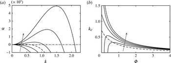
Variation of (a) perturbation growth rates
 $\unicode[STIX]{x1D6FC}$
for an initial thickness
 $\unicode[STIX]{x1D6F7}=0.1$
with the wavenumber
 $k$
and (b) cutoff wavenumbers
 $k_{c}$
with
 $\unicode[STIX]{x1D6F7}$
. With the dash-dotted line indicating the
 $\unicode[STIX]{x1D6FC}=0$
level, the dashed line represents the case where
 $\unicode[STIX]{x1D6E5}=\unicode[STIX]{x1D6FF}=0$
and the solid lines each correspond to
 $\unicode[STIX]{x1D6E5}=1$
and
 $\unicode[STIX]{x1D6FF}=0.4$
, 0.2, 0,
 $-0.2$
and
 $-0.4$
(arrows indicate direction of increasing
 $\unicode[STIX]{x1D6FF}$
).

Positive and negative values of
 $\unicode[STIX]{x1D6FC}$
naturally indicate instability and stability, respectively, and the cutoff wavenumber
 $k_{c}$
at which
 $\unicode[STIX]{x1D6FC}=0$
is
 $$\begin{eqnarray}\displaystyle & \displaystyle k_{c}=\left(\frac{1/2+\unicode[STIX]{x1D6E5}^{2}}{(1+\unicode[STIX]{x1D6F7})^{3}}+\frac{\unicode[STIX]{x1D6FF}\unicode[STIX]{x1D6E5}}{\unicode[STIX]{x1D6F7}(1+\unicode[STIX]{x1D6F7})^{2}}\right)^{1/2}. & \displaystyle\end{eqnarray}$$
The time-averaged growth rates
 $\unicode[STIX]{x1D6FC}$
, for
 $\unicode[STIX]{x1D6F7}=0.1$
, are depicted in figure 1(a) and they exhibit a typical dependence on wavenumber, whereby stabilization due to surface tension and destabilization due to thermocapillary stresses enter as
 $k^{4}$
and
 $k^{2}$
terms, respectively. The parameters
 $\unicode[STIX]{x1D6E5}$
and
 $\unicode[STIX]{x1D6FF}$
clearly influence
 $\unicode[STIX]{x1D6FC}$
, as well as the cutoff wavelengths
 $k_{c}$
, which are presented as a function of the mean thermal thickness
 $\unicode[STIX]{x1D6F7}$
in figure 1(b). With
 $\unicode[STIX]{x1D6FF}=\unicode[STIX]{x1D6E5}=0$
,
 $k_{c}=2^{-1/2}$
at
 $\unicode[STIX]{x1D6F7}\rightarrow 0$
, and decays monotonically to zero due to diminished surface temperature variations at large
 $\unicode[STIX]{x1D6F7}$
. With
 $\unicode[STIX]{x1D6FF}=0$
, finite values of
 $\unicode[STIX]{x1D6E5}$
promote destabilization for all
 $k$
and
 $\unicode[STIX]{x1D6F7}$
. Stabilization, however, is promoted when
 $\unicode[STIX]{x1D6FF}$
has the opposite sign of
 $\unicode[STIX]{x1D6E5}$
, and small values of
 $\unicode[STIX]{x1D6F7}$
may even be stabilized completely, viz.,
 $k_{c}$
for
 $\unicode[STIX]{x1D6FF}=-0.4$
and
 $-0.2$
in figure 1(b).
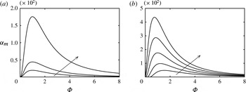
Dependence of maximum growth rates
 $\unicode[STIX]{x1D6FC}_{m}$
on the initial mean film thickness
 $\unicode[STIX]{x1D6F7}$
: (a)
 $-\unicode[STIX]{x1D6FF}=0$
with
 $\unicode[STIX]{x1D6E5}=0$
, 0.5, 1; (b)
 $-\unicode[STIX]{x1D6E5}=1.0$
with
 $\unicode[STIX]{x1D6FF}=0.4$
, 0.2, 0,
 $-0.2$
and
 $-0.4$
. The arrows in panels (a) and (b) indicate the directions of increasing
 $\unicode[STIX]{x1D6E5}$
and
 $\unicode[STIX]{x1D6FF}$
, respectively.

Next, we set
 $\unicode[STIX]{x2202}\unicode[STIX]{x1D6FC}/\unicode[STIX]{x2202}k=0$
and find that the fastest growing wavenumber is
 $k_{m}=2^{-1/2}k_{c}$
, which corresponds to a maximum growth rate of
 $\unicode[STIX]{x1D6FC}_{m}=(1/4)k_{c}^{4}\unicode[STIX]{x1D6F7}^{3}$
. For fixed values of
 $\unicode[STIX]{x1D6F7}$
,
 $\unicode[STIX]{x1D6FC}_{m}$
is presented in figure 2(a,b) for different values of
 $\unicode[STIX]{x1D6FF}$
and
 $\unicode[STIX]{x1D6E5}$
. Notably, for each case,
 $\unicode[STIX]{x1D6FC}_{m}$
approaches zero for small and large values of
 $\unicode[STIX]{x1D6F7}$
and, in between, attains a global maximum. This behaviour is a consequence of the form of the film temperature profile, which, using the current scaling, is
 $$\begin{eqnarray}\displaystyle \unicode[STIX]{x1D6E9}=\frac{\unicode[STIX]{x1D6E5}+\cos (\unicode[STIX]{x1D6FA}\unicode[STIX]{x1D70F})}{1+\unicode[STIX]{x1D719}}\unicode[STIX]{x1D701}, & & \displaystyle\end{eqnarray}$$
where
 $\unicode[STIX]{x1D701}=BZ$
. Accounting for this scaling and the definitions stated in (2.9), the dimensionless substrate temperature
 $\unicode[STIX]{x1D6E9}_{s}=0$
, the gas temperature
 $\tilde{\unicode[STIX]{x1D6E9}}_{g}=\bar{\unicode[STIX]{x1D6E9}}_{g}+\cos (\unicode[STIX]{x1D6FA}\unicode[STIX]{x1D70F})$
oscillates about the mean gas temperature
 $\bar{\unicode[STIX]{x1D6E9}}_{g}=\unicode[STIX]{x1D6E5}$
, and
 $\unicode[STIX]{x1D6E9}_{0}=-\unicode[STIX]{x1D6FF}$
corresponds to the temperature
 $\unicode[STIX]{x1D703}_{0}$
that yields the minimum surface tension
 $\unicode[STIX]{x1D70E}_{0}$
. As
 $\unicode[STIX]{x1D719}=\unicode[STIX]{x1D6F7}$
approaches zero, the surface temperature
 $\unicode[STIX]{x1D6E9}(\unicode[STIX]{x1D701}=\unicode[STIX]{x1D719})$
tends therefore uniformly to the substrate temperature. Hence, the thermocapillary stresses are negligible and the growth rate is zero. Likewise,
 $\unicode[STIX]{x1D6FC}_{m}$
is zero for large values of
 $\unicode[STIX]{x1D6F7}$
, under which conditions the film surface temperature is uniformly equal to the gas temperature
 $\tilde{\unicode[STIX]{x1D6E9}}_{g}=\unicode[STIX]{x1D6E5}+\cos (\unicode[STIX]{x1D6FA}\unicode[STIX]{x1D70F})$
. A trade-off therefore exists between the gas–liquid heat transfer rate and the film thickness, which leads to a global maximum growth rate
 $\unicode[STIX]{x1D6FC}_{g}$
at a specific value
 $\unicode[STIX]{x1D6F7}=\unicode[STIX]{x1D6F7}_{g}$
for any given values of
 $\unicode[STIX]{x1D6E5}$
and
 $\unicode[STIX]{x1D6FF}$
. The global
 $\unicode[STIX]{x1D6FC}_{g}$
occurs at
 $\unicode[STIX]{x1D6F7}_{g}=1$
for all cases where
 $\unicode[STIX]{x1D6FF}=0$
, and shifts to
 $\unicode[STIX]{x1D6F7}_{g}$
are introduced by setting finite
 $\unicode[STIX]{x1D6FF}$
and
 $\unicode[STIX]{x1D6E5}$
, as seen in panels 2(a) and 2(b), respectively.
Physical aspects of the preceding analysis will now be discussed by considering the evolution of the surface tension for local values of the film height
 $\unicode[STIX]{x1D719}$
. To do so, we first non-dimensionalize (2.4), which gives
 $$\begin{eqnarray}\displaystyle \unicode[STIX]{x1D70E}=\unicode[STIX]{x1D70E}_{0}+\unicode[STIX]{x1D6FE}\hat{\unicode[STIX]{x1D703}}_{g}^{2}(\unicode[STIX]{x1D6E9}+\unicode[STIX]{x1D6FF})^{2} & & \displaystyle\end{eqnarray}$$
and is valid at the interface
 $\unicode[STIX]{x1D701}=\unicode[STIX]{x1D719}$
. Then we substitute the temperature profile
 $\unicode[STIX]{x1D6E9}(\unicode[STIX]{x1D701}=\unicode[STIX]{x1D719})$
into (3.7), and define a non-dimensional correction to the local surface tension
 $S(\unicode[STIX]{x1D70F},\unicode[STIX]{x1D719})$
as
 $$\begin{eqnarray}\displaystyle S=\frac{\unicode[STIX]{x1D70E}-\unicode[STIX]{x1D70E}_{0}}{\unicode[STIX]{x1D6FE}\hat{\unicode[STIX]{x1D703}}_{g}^{2}}=\left(\frac{\unicode[STIX]{x1D6E5}+\cos (\unicode[STIX]{x1D6FA}\unicode[STIX]{x1D70F})}{1+\unicode[STIX]{x1D719}}\unicode[STIX]{x1D719}+\unicode[STIX]{x1D6FF}\right)^{2}, & & \displaystyle\end{eqnarray}$$
which has a time-averaged component
 $$\begin{eqnarray}\displaystyle \bar{S}=\frac{1/2+\unicode[STIX]{x1D6E5}^{2}}{(1+\unicode[STIX]{x1D719})^{2}}\unicode[STIX]{x1D719}^{2}+\frac{2\unicode[STIX]{x1D6FF}\unicode[STIX]{x1D6E5}}{1+\unicode[STIX]{x1D719}}\unicode[STIX]{x1D719}+\unicode[STIX]{x1D6FF}^{2}. & & \displaystyle\end{eqnarray}$$
In the following discussion, the evolution of
 $S$
throughout an excitation period will be considered for different cases of (
 $\unicode[STIX]{x1D6FF}$
,
 $\unicode[STIX]{x1D6E5}$
) that are representative of cases (i)–(iv). To highlight the instantaneous and time-averaged Marangoni stresses that drive film dynamics, we consider the values of
 $S$
and
 $\bar{S}$
evaluated at
 $\unicode[STIX]{x1D719}=\unicode[STIX]{x1D719}_{1}=0.8$
(representative of a trough) and
 $\unicode[STIX]{x1D719}_{2}=1.0$
(crest). Accordingly, to simplify notation, we denote the trough and crest values of
 $S$
and
 $\bar{S}$
as
 $S_{1}=S(\unicode[STIX]{x1D719}_{1})$
and
 $\bar{S}_{1}=\bar{S(\unicode[STIX]{x1D719}_{1})}$
, and
 $S_{2}=S(\unicode[STIX]{x1D719}_{2})$
and
 $\bar{S}_{2}=\bar{S(\unicode[STIX]{x1D719}_{2})}$
, respectively. We note that the following discussion is highly nuanced, and it may be sufficient for the reader to only consider that pertaining to case (i), which is the focus of the nonlinear study in § 4. The discussion of cases (ii)–(iv) in this section can then be considered to infer behaviour in more complex experimental settings, which we discuss in § 5.
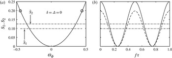
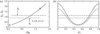
Evolution of non-dimensional surface tension at a trough,
 $S_{1}$
(solid lines in both panels), and at a crest,
 $S_{2}$
, with respect to (a) surface temperature and (b) time for
 $(\unicode[STIX]{x1D6FF},\unicode[STIX]{x1D6E5})=(0,0)$
. In panel (a),
 $S_{1}$
traces the path along
 $S_{2}$
and its endpoints have been marked by circles. In panel (b),
 $S_{1}$
is given by the dashed line. In both panels, dash-dotted lines are used to indicate time-averaged values of
 $\bar{S}_{1}=0.099$
and
 $\bar{S}_{2}=0.125$
as labelled.

The evolution of
 $S_{1}$
and
 $S_{2}$
for case (i), with
 $\unicode[STIX]{x1D6FF}=\unicode[STIX]{x1D6E5}=0$
, is presented throughout the excitation in figure 3(a,b) as functions of the temporally evolving surface temperature
 $\unicode[STIX]{x1D6E9}_{\unicode[STIX]{x1D719}}$
and the time coordinate
 $f\unicode[STIX]{x1D70F}$
, respectively. At time
 $f\unicode[STIX]{x1D70F}=0$
, the gas temperature
 $\tilde{\unicode[STIX]{x1D6E9}}_{g}=1$
is higher than the substrate temperature
 $\unicode[STIX]{x1D6E9}_{s}=0$
, and, via (3.8),
 $S$
is an increasing function of
 $\unicode[STIX]{x1D719}$
. Therefore, instantaneously, a surface traction drives flow from a thinner location of the interface to a thicker one, e.g. from
 $\unicode[STIX]{x1D719}_{1}$
to
 $\unicode[STIX]{x1D719}_{2}$
. As time proceeds,
 $\tilde{\unicode[STIX]{x1D6E9}}_{g}$
and
 $S_{2}-S_{1}$
decrease until they vanish at
 $f\unicode[STIX]{x1D70F}=1/4$
, at which point the system temperature is uniformly equal to
 $\tilde{\unicode[STIX]{x1D6E9}}_{g}=0$
. The reverse process occurs during
 $1/4\leqslant f\unicode[STIX]{x1D70F}\leqslant 1/2$
, whereby
 $S_{2}-S_{1}$
increases from 0 to its maximal value and
 $\tilde{\unicode[STIX]{x1D6E9}}_{g}$
continues to decrease from 0 to
 $-1$
. Then, the evolution of
 $S_{2}-S_{1}$
during the gas cooling cycle is repeated during the subsequent warming cycle that occurs for
 $1/2\leqslant f\unicode[STIX]{x1D70F}\leqslant 1$
as
 $\tilde{\unicode[STIX]{x1D6E9}}_{g}$
increases from
 $-1$
to 1. At no point during the excitation are the surface tractions directed from crest to trough for case (i), which would promote stabilization. As a result, there exists a time-averaged flow from crest to trough that destabilizes domains of wavenumbers
 $k<k_{c}$
as depicted in figure 1(a). The destabilization process is
 $2\unicode[STIX]{x1D6FA}$
-periodic for case (i), due to the symmetry of the surface tension with respect to the thermal fluctuations. In general, the destabilizations associated with cases (ii)–(iv) contain both
 $\unicode[STIX]{x1D6FA}$
and
 $2\unicode[STIX]{x1D6FA}$
components.
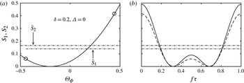
Evolution of non-dimensional surface tension at a trough,
 $S_{1}$
, and at a crest,
 $S_{2}$
, with respect to (a) surface temperature and (b) time for
 $(\unicode[STIX]{x1D6FF},\unicode[STIX]{x1D6E5})=(0.2,0)$
. All curve and point designations are as in figure 3. In both panels, the dash-dotted lines indicate time-averaged values of
 $\bar{S}_{1}=0.139$
and
 $\bar{S}_{2}=0.165$
as labelled.

Case (ii) describes the configuration where the substrate and mean gas temperatures are held equal (
 $\unicode[STIX]{x1D6E5}=0$
) to a value that may either be higher (positive
 $\unicode[STIX]{x1D6FF}$
) or lower (negative
 $\unicode[STIX]{x1D6FF}$
) than
 $\unicode[STIX]{x1D703}_{0}$
, which, in scaled units, is equal to
 $-\unicode[STIX]{x1D6FF}$
. Positive and negative values of
 $\unicode[STIX]{x1D6FF}$
therefore bias the excitation towards higher and lower temperatures than that described by case (i). Figure 4(a,b) depicts the evolution of
 $S_{2}$
and
 $S_{1}$
during an excitation period where
 $\unicode[STIX]{x1D6E5}=0$
and
 $\unicode[STIX]{x1D6FF}=0.2$
. Clearly, the bias breaks the symmetry of the excitation with respect to
 $\unicode[STIX]{x1D703}_{0}$
, which leads to the introduction of an
 $\unicode[STIX]{x1D6FA}$
linear response frequency in addition to the
 $2\unicode[STIX]{x1D6FA}$
response. Nevertheless, this bias does not change the difference between
 $\bar{S}$
for two different values of
 $\unicode[STIX]{x1D719}$
and as a result the cutoff wavelength
 $k_{c}$
does not depend upon
 $\unicode[STIX]{x1D6FF}$
for
 $\unicode[STIX]{x1D6E5}=0$
, as follows from equation (3.5).
Evolution of non-dimensional surface tensions at a trough,
 $S_{1}$
, and at a crest,
 $S_{2}$
, with respect to (a) surface temperature and (b) time for
 $(\unicode[STIX]{x1D6FF},\unicode[STIX]{x1D6E5})=(0,2)$
. All curve and point designations are as in figure 3. In both panels, the dash-dotted lines indicate time-averaged values of
 $\bar{S}_{1}=0.89$
and
 $\bar{S}_{2}=1.13$
as labelled.

For case (iii), the substrate temperature is held at
 $\unicode[STIX]{x1D703}_{0}$
(
 $\unicode[STIX]{x1D6FF}=0$
) and is heated (negative
 $\unicode[STIX]{x1D6E5}$
) or cooled (positive
 $\unicode[STIX]{x1D6E5}$
) with respect to the mean gas temperature. As in case (ii), the film surface is biased towards temperatures that are either warmer or cooler than
 $\unicode[STIX]{x1D703}_{0}$
. However, via (3.6), heating or cooling magnifies the temperature differences between a crest and a trough throughout the excitation. As a result,
 $\unicode[STIX]{x1D6FC}$
and
 $k_{c}$
are increased for all
 $\unicode[STIX]{x1D6F7}$
. Also observe that the film surface temperature can be set to reside entirely above (or below)
 $\unicode[STIX]{x1D703}_{0}$
by increasing the magnitude of heating/cooling larger than the modulation amplitude, i.e.
 $|\unicode[STIX]{x1D6E5}|>1$
. The evolution of
 $S$
is depicted for such a configuration in figure 5 with
 $(\unicode[STIX]{x1D6FF},\unicode[STIX]{x1D6E5})=(0,2)$
and shows that the
 $2\unicode[STIX]{x1D6FA}$
response is diminished significantly because the surface tension minimum is not traversed.
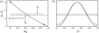
Evolution of non-dimensional surface tensions at a trough,
 $S_{1}$
, and at a crest,
 $S_{2}$
, with respect to (a) surface temperature and (b) time for
 $(\unicode[STIX]{x1D6FF},\unicode[STIX]{x1D6E5})=(-2,1)$
. All curve and point designations are as in figure 3. In both panels, the dash-dotted lines indicate time-averaged values of
 $\bar{S}_{1}=2.52$
and
 $\bar{S}_{2}=2.38$
as labelled.

Finally, for case (iv), both
 $\unicode[STIX]{x1D6FF}$
and
 $\unicode[STIX]{x1D6E5}$
take finite values, which represents the combination of thermal modulation with steady heating/cooling, for substrate temperatures set away from
 $\unicode[STIX]{x1D703}_{0}$
. From (3.3), it is clear that positive/negative values of
 $\unicode[STIX]{x1D6FF}\unicode[STIX]{x1D6E5}$
promote instability/stability via the second term in the parentheses. This term describes the thermocapillary effects due to steady heating/cooling that depend linearly on the surface temperature, and arises when the system is biased towards temperatures above or below
 $\unicode[STIX]{x1D703}_{0}$
. For example, when
 $\unicode[STIX]{x1D6FF}<0$
, the system is biased towards temperatures that are less than
 $\unicode[STIX]{x1D703}_{0}$
, where surface tension is a decreasing function of temperature. In this region, uniform substrate heating (negative
 $\unicode[STIX]{x1D6E5}$
) is destabilizing, as is the case for typical fluids whose surface tension decreases (linearly) with temperature, see Oron et al. (Reference Oron, Davis and Bankoff1997). Contrary to typical fluids, films with surface tension minima may also be destabilized by uniform substrate cooling (negative
 $\unicode[STIX]{x1D6E5}$
) when the system is biased towards temperatures higher than
 $\unicode[STIX]{x1D703}_{0}$
(positive
 $\unicode[STIX]{x1D6FF}$
), where surface tension is an increasing function of temperature. The contribution of these linear thermocapillary effects must nevertheless compete with those given by the first term in the parentheses of (3.3), which depends quadratically on the surface temperature. It is worth noting that, at small values of
 $\unicode[STIX]{x1D6F7}$
, the linear thermocapillary contribution to
 $\unicode[STIX]{x1D6FC}$
is
 $\mathit{O}(\unicode[STIX]{x1D6F7}^{2})$
and therefore dominates both the quadratic thermocapillary and surface tension contributions, which are
 $\mathit{O}(\unicode[STIX]{x1D6F7}^{3})$
. As a result, we find that the cutoff wavenumber diverges as
 $\unicode[STIX]{x1D6F7}\rightarrow$
0 for increasing positive values of
 $\unicode[STIX]{x1D6FF}\unicode[STIX]{x1D6E5}$
, see
 $k_{c}$
for
 $(\unicode[STIX]{x1D6E5},\unicode[STIX]{x1D6FF})=(1,0.2)$
and (1,0.4) in figure 1(b). Alternatively, when the product
 $\unicode[STIX]{x1D6FF}\unicode[STIX]{x1D6E5}$
is negative, steady heating/cooling can stabilize the film completely as
 $\unicode[STIX]{x1D6F7}\rightarrow$
0, as depicted by
 $k_{c}$
for
 $(\unicode[STIX]{x1D6E5},\unicode[STIX]{x1D6FF})=(1,-0.2)$
and (
 $1,-0.4$
). An example of such a configuration, which leads to a time-averaged value of
 $\bar{S}_{2}<\bar{S}_{1}$
, is given in figure 6.
To summarize, modulation of the gas temperature alone can destabilize a film that is otherwise held at isothermal conditions, due to quadratic dependence of surface tension on temperature. The cutoff wavelengths
 $k_{c}$
and time-averaged growth rates
 $\unicode[STIX]{x1D6FC}$
depend upon the arrangement of the thermal boundary conditions via
 $\unicode[STIX]{x1D6FF}$
and
 $\unicode[STIX]{x1D6E5}$
as well as the mean thermal thickness
 $\unicode[STIX]{x1D6F7}$
. Considering that system dynamics is equivalent under the transformation
 $(\unicode[STIX]{x1D6E5},\unicode[STIX]{x1D6FF},f\unicode[STIX]{x1D70F})\rightarrow (-\unicode[STIX]{x1D6E5},-\unicode[STIX]{x1D6FF},f\unicode[STIX]{x1D70F}+1)$
, figure 1 conclusively presents the behaviour of
 $k_{c}$
with respect to this parameter space. Although
 $\unicode[STIX]{x1D6FA}$
does not affect linear stability it will be seen in the next section to bear critical importance on the emergence of saturated nonlinear flows.
4 Numerical study
We proceed with a numerical investigation of initially flat films described by (2.17) on spatially periodic domains, aiming to provide insight into strongly nonlinear regimes. The numerical method is identical to that used by Batson et al. (Reference Batson, Agnon and Oron2015) in their investigation of hanging films subject to thermal excitation by acoustic waves. In summary, a Fourier collocation method is used to discretize space and build appropriate differentiation operators (Boyd Reference Boyd2001). An explicit integration scheme for the evaluation of the increment in the interface profile
 $\unicode[STIX]{x1D719}(\unicode[STIX]{x1D709},\unicode[STIX]{x1D70F})$
in time is used via a first-order forward Euler method with time step
 $\unicode[STIX]{x1D6E5}\unicode[STIX]{x1D70F}$
and Newton–Kantorovich linearization of the nonlinearities (Haimovich & Oron Reference Haimovich and Oron2010). Numerical analysis of time series at the excitation frequency is supported by setting the number of time steps per excitation period to an integer number. Of particular interest are saturated flows, which we classify as those numerical solutions for which the
 $L_{2}$
norm of
 $\unicode[STIX]{x1D719}$
changes by less than
 $1\times 10^{-8}$
after an excitation period. It will be demonstrated that saturated, non-rupturing flows emerge when
 $\unicode[STIX]{x1D6FA}$
is the same order as the linear growth rate
 $\unicode[STIX]{x1D6FC}$
. Mainly we focus on these values of
 $\unicode[STIX]{x1D6FA}$
, and, in the results that follow, convergence is typically obtained by using 128 Fourier modes and between 300 and 400 time steps per period. Whereas some integrations of (2.17) are initialized with small perturbations to flat films, for example,
 $\unicode[STIX]{x1D719}(\unicode[STIX]{x1D709},\unicode[STIX]{x1D70F}=0)=\unicode[STIX]{x1D6F7}+0.001\cos k\unicode[STIX]{x1D709}$
, solution branches are also tracked by continuation with respect to small changes in the independent parameters by initializing computations with nearby saturated solutions. Finally, we restrict our interest in the following numerical study to case (i), that is, a film that is thermally modulated about its mean temperature, which is fixed to
 $\unicode[STIX]{x1D703}_{0}$
. In doing so, the parameter space is reduced significantly and permits a thorough investigation of the dynamics induced solely by modulation about
 $\unicode[STIX]{x1D703}_{0}$
.
4.1 General nonlinear dynamics
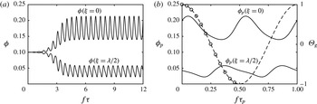
Time evolution of
 $\unicode[STIX]{x1D719}(\unicode[STIX]{x1D709}=0)$
and
 $\unicode[STIX]{x1D719}(\unicode[STIX]{x1D709}=\unicode[STIX]{x1D706}/2)$
with
 $(\unicode[STIX]{x1D6F7},k,\unicode[STIX]{x1D6FF},\unicode[STIX]{x1D6E5},\unicode[STIX]{x1D6FA})=(0.1,0.55,0,0,2\unicode[STIX]{x1D6FC}_{m})$
, where
 $\unicode[STIX]{x1D706}=2\unicode[STIX]{x03C0}/k$
. Panels (a) and (b) depict saturation from an initial condition
 $\unicode[STIX]{x1D719}(\unicode[STIX]{x1D70F}=0)=\unicode[STIX]{x1D6F7}+0.001\cos k\unicode[STIX]{x1D709}$
and the saturated dynamics of
 $\unicode[STIX]{x1D719}_{p}$
for a single excitation period following the saturation state, respectively. The gas temperature
 $\tilde{\unicode[STIX]{x1D6E9}}_{g}$
is superimposed on panel (b), and the circles indicate values for which full profiles of
 $\unicode[STIX]{x1D719}_{p}$
are given in figure 8.


The dynamics of a perturbation with linearly unstable wavelength is depicted for case (i) in figures 7 and 8 where
 $(\unicode[STIX]{x1D6F7},k,\unicode[STIX]{x1D6FF},\unicode[STIX]{x1D6E5},\unicode[STIX]{x1D6FA})=(0.1,0.55,0,0,2\unicode[STIX]{x1D6FC}_{m})$
and
 $\unicode[STIX]{x1D6FC}_{m}=3.53\times 10^{-5}$
. In figure 7(a), the evolution of the film thickness at
 $\unicode[STIX]{x1D709}=0$
and the domain midpoint
 $\unicode[STIX]{x1D709}=\unicode[STIX]{x1D706}/2$
clearly demonstrate growth and saturation to a regular time-periodic flow. Note that
 $\unicode[STIX]{x1D706}=2\unicode[STIX]{x03C0}/k$
is the wavelength of the periodic domain. The nonlinear saturation to a non-rupturing profile can be described as follows.
First, observe for any profile
 $\unicode[STIX]{x1D719}=\unicode[STIX]{x1D719}(\unicode[STIX]{x1D709},\unicode[STIX]{x1D70F})$
, that the interface temperature is uniformly
 $\unicode[STIX]{x1D6E9}(\unicode[STIX]{x1D701}=\unicode[STIX]{x1D719})=0$
whenever
 $\cos \unicode[STIX]{x1D6FA}\unicode[STIX]{x1D70F}=0$
, viz. (3.6). At this moment, Marangoni stresses are completely absent from the interface, and surface tension will act to stabilize any deflections. The subsequent increase (or decrease) of
 $\tilde{\unicode[STIX]{x1D6E9}}_{g}$
reintroduces Marangoni stresses to the film, and the profile will be locally destabilized once the local effect of surface tension is surpassed. The maximum driving force for destabilization naturally occurs when
 $|\text{cos}\unicode[STIX]{x1D6FA}\unicode[STIX]{x1D70F}|=1$
. In the nonlinear regime, the thermal gas excitation therefore generates intermittent stabilization–destabilization with strong dependence on the local value of
 $\unicode[STIX]{x1D719}$
and its horizontal derivatives. Because of the slower time scales associated with smaller values of
 $\unicode[STIX]{x1D719}$
, it is possible for a balance to be struck between the stabilization and destabilization cycles of a deflected film over a period of the excitation. Saturation generally occurs when
 $\unicode[STIX]{x1D6FA}$
is of the same order as
 $\unicode[STIX]{x1D6FC}$
. If
 $\unicode[STIX]{x1D6FA}$
is too small, then the film ruptures because the destabilization cycle is too long. On the other hand, if
 $\unicode[STIX]{x1D6FA}$
is too large, the film ruptures because the stabilization cycle is too short and the film cannot respond to exceedingly fast excitation.
4.2 Periodic flow
At sufficiently long times, and to within numerical tolerance, the time series of figure 7(a) saturate to
 $2\unicode[STIX]{x1D6FA}$
time-periodic flows. It is useful to consider these series to be periodic functions
 $\unicode[STIX]{x1D719}_{p}$
that satisfy
 $\displaystyle \unicode[STIX]{x1D719}_{p}(f\unicode[STIX]{x1D70F}_{p})=\unicode[STIX]{x1D719}_{p}((n/2)f\unicode[STIX]{x1D70F}_{p})$
for integers
 $n$
. We specify that the shifted time coordinate
 $f\unicode[STIX]{x1D70F}_{p}=0$
is initialized at a time
 $\unicode[STIX]{x1D70F}$
when
 $\cos \unicode[STIX]{x1D6FA}\unicode[STIX]{x1D70F}=1$
. With these definitions, different periodic flows
 $\unicode[STIX]{x1D719}_{p}$
can be conveniently analysed and compared on the interval of a half-excitation period, that is,
 $0\leqslant f\unicode[STIX]{x1D70F}_{p}<1/2$
, where
 $0\leqslant \unicode[STIX]{x1D70F}_{p}<\unicode[STIX]{x03C0}/\unicode[STIX]{x1D6FA}$
. In figure 7(b), the periodic functions
 $\unicode[STIX]{x1D719}_{p}$
obtained from the calculation of panel (a) are superimposed with a single excitation period of the gas temperature. Here one observes phase lags in both
 $\unicode[STIX]{x1D719}_{p}(\unicode[STIX]{x1D709}=0)$
and
 $\unicode[STIX]{x1D719}_{p}(\unicode[STIX]{x1D709}=\unicode[STIX]{x1D706}/2)$
with respect to
 $\tilde{\unicode[STIX]{x1D6E9}}_{g}$
because both continue to increase and decrease, respectively, after the driving force for destabilization is maximized at
 $\unicode[STIX]{x1D70F}_{p}=0$
.
In fact,
 $\unicode[STIX]{x1D719}$
is found to approach
 $2\unicode[STIX]{x1D6FA}$
periodicity for all locations
 $\unicode[STIX]{x1D709}$
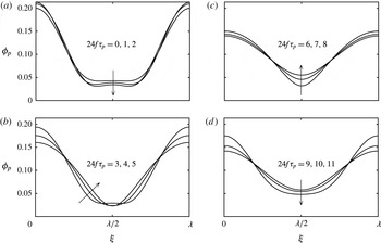
after a long time in the calculation of figure 7. The associated film profiles,
 $\unicode[STIX]{x1D719}_{p}$
, are given in figure 8(a–d), at times corresponding to the circles marked on
 $\tilde{\unicode[STIX]{x1D6E9}}_{g}$
in figure 7(b). In panel (a), it is seen in the time immediately following the maximum
 $\tilde{\unicode[STIX]{x1D6E9}}_{g}=1$
that the crest continues to grow, and the trough deepens via a secondary instability that generates a secondary hump at
 $\unicode[STIX]{x1D719}(\unicode[STIX]{x1D709}=\unicode[STIX]{x1D706}/2)$
. In panel (b),
 $\tilde{\unicode[STIX]{x1D6E9}}_{g}$
decreases further towards zero, thereby minimizing the Marangoni surface stresses and promoting stabilization – first at the profile crest followed by the trough, as confirmed by the phase lags in figure 7(b). In panel (c),
 $\tilde{\unicode[STIX]{x1D6E9}}_{g}$
starts at the minimum temperature of zero, and the film continues to stabilize until
 $\tilde{\unicode[STIX]{x1D6E9}}_{g}$
becomes sufficiently negative in panel (d). Due to the symmetry of the surface tension with respect to oscillations of
 $\tilde{\unicode[STIX]{x1D6E9}}_{g}$
, the dynamics of the film during the subsequent heating cycle, where
 $\tilde{\unicode[STIX]{x1D6E9}}_{g}$
increases from
 $-1$
to 1, is identical to that depicted for the cooling cycle in figure 8, where
 $\tilde{\unicode[STIX]{x1D6E9}}_{g}$
decreases from 1 to
 $-1$
.
4.3 Streamlines
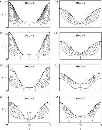
A more detailed view of the periodic stabilization–destabilization process is provided by the streamlines, which have been drawn using (2.18) for the flow of figures 7 and 8 in figure 9(a–h) for times
 $16f\unicode[STIX]{x1D70F}_{p}=0$
, 1, 2, 3, 4, 5, 6 and 7, respectively, (note that a time interval different from figures 7 and 8 has been used). Vertical streamlines with
 $\unicode[STIX]{x1D713}=0$
exist on the boundaries and the midpoint of the periodic domain, for all values of
 $\unicode[STIX]{x1D701}$
(or
 $Z$
), because both
 $\unicode[STIX]{x1D719}_{\unicode[STIX]{x1D709}}=0$
and
 $\unicode[STIX]{x1D719}_{\unicode[STIX]{x1D709}\unicode[STIX]{x1D709}\unicode[STIX]{x1D709}}=0$
at these locations throughout the excitation. These streamlines ensure that the flow is composed of at least two convection cells that are symmetric with respect to either
 $\unicode[STIX]{x1D709}=0$
or
 $\unicode[STIX]{x1D706}/2$
, evident by the opposite signs of
 $\unicode[STIX]{x1D713}$
in adjacent cells.
Flow streamlines
 $\unicode[STIX]{x1D713}\times 10^{6}$
for
 $\unicode[STIX]{x1D719}_{p}$
at evenly spaced times from
 $16f\unicode[STIX]{x1D70F}_{p}=0$
to 7, corresponding to the parameter set from figure 7. Positive and negative values of the streamfunction correspond to counterclockwise and clockwise flow along the streamlines, respectively.

Except for panels (e) and (f), these cells are divided further by additional
 $\unicode[STIX]{x1D713}=0$
streamlines that change location as time proceeds. Observe in panel (a) for
 $16f\unicode[STIX]{x1D70F}_{p}=0$
that the
 $\unicode[STIX]{x1D713}=0$
streamlines that bound the lower left and lower right cells from above do not terminate at the interface, and that all the streamlines contained within these cells form closed loops, indicating vortical flow. On the other hand, the middle of two convection cells depicted in panel (a) contain open streamlines that terminate at the film interface, which implies that the velocity of the film interface is finite. At this moment we know from figures 7(b) and 8(a) that the interfacial deflection is growing, and therefore these open streamlines represent flows that draw fluid from trough to crest. We therefore refer to the cells that contain open streamlines in panel (a) of figure 9 as destabilization cells.
In the next frame at
 $16\unicode[STIX]{x1D70F}_{p}=1$
in panel (b), the flow intensity and size of the destabilization cells have decreased, at the expense of growing cells that were purely vortical in panel (a). In panel (b), the cells which have grown now contain open streamlines and act as stabilization cells that draw fluid from crest to trough. In the following two panels (c) and (d), the stabilization cells continue to grow, until the destabilization cells have vanished completely, as seen at
 $16f\unicode[STIX]{x1D70F}_{p}=4$
in panel (e). Then, for times
 $5<16f\unicode[STIX]{x1D70F}_{p}<6$
, destabilization cells (with open streamlines) reappear on the film crest and grow until the stabilization cells (with closed streamlines) are pushed entirely below the film surface, viz., panel (g) at
 $16f\unicode[STIX]{x1D70F}_{p}=6$
. The destabilization cells are larger in panel (h) at
 $16f\unicode[STIX]{x1D70F}_{p}=7$
, as expected, and the process resets to figure 9(a) for
 $16f\unicode[STIX]{x1D70F}_{p}=8$
.
To summarize, the periodic flow
 $\unicode[STIX]{x1D719}_{p}$
is composed of the emergence and disappearance of stabilization and destabilization cells. At certain times, the open streamlines contacting the interface belong strictly to destabilization/stabilization cells, during which the deflection grows/decays across the entire domain. During the other parts of the excitation, the interface is contacted by open streamlines belonging to both stabilization and destabilization cells, which results in separated regions of deflection growth and decay within the domain, viz., figure 9(b,c).
It is instructive to contrast this flow to those investigated by Oron & Rosenau (Reference Oron and Rosenau1994), because only they have previously considered flow of films with quadratic surface tension. Instead of time-periodic excitation, their flow is driven by substrate heating or cooling when the respective substrate and gas temperatures span
 $\unicode[STIX]{x1D703}_{0}$
. Notably, their flow is characterized by vortical destabilization and stabilization cells located about the film crests and troughs, respectively. The vertical boundary between these cells connects to a stagnation point on the interface, at which the temperature is equal to
 $\unicode[STIX]{x1D703}_{0}$
, and the profile is therefore maintained by Marangoni stresses that emanate from this point, in opposite directions. The flows investigated in the nonlinear section of this work, on the other hand, are driven by Marangoni stresses that are always directed from trough to crest and
 $\unicode[STIX]{x1D703}_{0}$
is reached uniformly on the film interface only when
 $\cos \unicode[STIX]{x1D6FA}\unicode[STIX]{x1D70F}=0$
. Furthermore, the dynamics of destabilization/stabilization cells is significantly more complex and depends on the instantaneous Marangoni and capillary stresses.
4.4 The effect of
 $\unicode[STIX]{x1D6FA}$

Influence of
 $\unicode[STIX]{x1D6FA}$
on
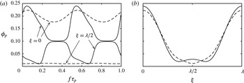
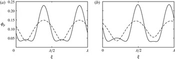
 $\unicode[STIX]{x1D719}_{p}(\unicode[STIX]{x1D709},\unicode[STIX]{x1D70F}_{p})$
for
 $(\unicode[STIX]{x1D6F7},k,\unicode[STIX]{x1D6FF},\unicode[STIX]{x1D6E5})=(0.1,0.55,0,0)$
. Panel (a) depicts the evolution of
 $\unicode[STIX]{x1D719}_{p}$
at
 $\unicode[STIX]{x1D709}=0$
and the domain midpoint
 $\unicode[STIX]{x1D709}=\unicode[STIX]{x1D706}/2$
across an excitation period for
 $\unicode[STIX]{x1D6FA}=0.4\unicode[STIX]{x1D6FC}_{m}$
(solid lines) and
 $10\unicode[STIX]{x1D6FC}_{m}$
(dashed lines). The profiles for which
 $|\unicode[STIX]{x1D719}_{p}|$
is maximized are given in panel (b) for
 $\unicode[STIX]{x1D6FA}=0.4\unicode[STIX]{x1D6FC}_{m}$
(solid line) and
 $\unicode[STIX]{x1D6FA}=10\unicode[STIX]{x1D6FC}_{m}$
(dashed line) and occur at
 $f\unicode[STIX]{x1D70F}_{p}=0.056$
and 0.067, respectively.

The relation between
 $\unicode[STIX]{x1D6FA}$
and the film growth/decay and its influence on the evolution of
 $\unicode[STIX]{x1D719}_{p}(\unicode[STIX]{x1D709},\unicode[STIX]{x1D70F}_{p})$
is presented in figure 10, where, save for
 $\unicode[STIX]{x1D6FA}$
, the parameter values are identical to the results presented in figures 7–9. In panel (a), the solid lines depict the evolution of
 $\unicode[STIX]{x1D719}_{p}$
at
 $\unicode[STIX]{x1D709}=0$
and
 $\unicode[STIX]{x1D706}/2$
for
 $\unicode[STIX]{x1D6FA}=0.4\unicode[STIX]{x1D6FC}_{m}$
. Compared to figure 7(b), the most striking feature is that the longer stabilization period (lower
 $\unicode[STIX]{x1D6FA}$
) results in almost complete stabilization of the film to a flat state, which is depicted here by the decay of
 $\unicode[STIX]{x1D719}_{p}$
to the initial value of 0.1 for both the major crest and trough. The evolution of
 $\unicode[STIX]{x1D719}_{p}$
at these locations is also presented by the dashed curves for much larger
 $\unicode[STIX]{x1D6FA}=10\unicode[STIX]{x1D6FC}_{m}$
in figure 10(a), and, as in figure 7(b), the frequency is too large for the film deflections to be completely stabilized. The dependence of the nonlinear growth/decay on the local thickness is especially clear for
 $\unicode[STIX]{x1D6FA}=10\unicode[STIX]{x1D6FC}_{m}$
by noting that the amplitude of the film trough oscillation is almost negligible compared to that of the crest. It is the combination of this effect with the intermittency of the destabilization that allows for the emergence of saturated flows. Another qualitative effect of
 $\unicode[STIX]{x1D6FA}$
is presented in panel (b), where the full profiles
 $\unicode[STIX]{x1D719}_{p}$
are depicted for both frequencies at times
 $f\unicode[STIX]{x1D70F}_{p}$
where
 $|\unicode[STIX]{x1D719}_{p}|$
is maximal. Whereas the secondary hump is present in the profile for
 $\unicode[STIX]{x1D6FA}=0.4\unicode[STIX]{x1D6FC}_{m}$
, it is conspicuously absent from the
 $\unicode[STIX]{x1D6FA}=10\unicode[STIX]{x1D6FC}_{m}$
profile. Because this secondary destabilization occurs on a longer time scale than the primary instability, we generally find that these secondary humps vanish for any
 $\unicode[STIX]{x1D719}_{p}$
when
 $\unicode[STIX]{x1D6FA}$
is increased sufficiently.
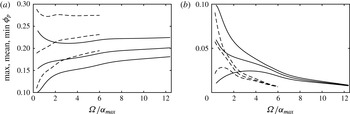
Influence of
 $\unicode[STIX]{x1D6FA}$
on the maximum, mean and minimum values of
 $\unicode[STIX]{x1D719}_{p}(\unicode[STIX]{x1D709},\unicode[STIX]{x1D70F})$
attained throughout an excitation period of the film thicknesses (a)
 $\unicode[STIX]{x1D719}_{p}(\unicode[STIX]{x1D709}=0)$
and (b)
 $\unicode[STIX]{x1D719}_{p}(\unicode[STIX]{x1D709}=\unicode[STIX]{x1D706}/2)$
for
 $k=0.55$
(solid lines) and 0.45 (dashed lines).

The general effect of
 $\unicode[STIX]{x1D6FA}$
is summarized in figure 11, where the local maximum, mean and minimum values attained by
 $\unicode[STIX]{x1D719}_{p}$
during an excitation period are given for the domain edge
 $\unicode[STIX]{x1D709}=0$
in panel (a) and the midpoint
 $\unicode[STIX]{x1D709}=\unicode[STIX]{x1D706}/2$
in panel (b). These values are tracked continuously with respect to
 $\unicode[STIX]{x1D6FA}$
for wavenumbers
 $k=0.55$
and 0.45. The tendency towards periods of complete film stabilization, at low frequencies, is evident from the approach of the minimum value
 $\unicode[STIX]{x1D719}_{p}(\unicode[STIX]{x1D709}=0)$
and the maximum value of
 $\unicode[STIX]{x1D719}_{p}(\unicode[STIX]{x1D709}=\unicode[STIX]{x1D706}/2)$
to 0.1 as frequency is decreased, for both values of
 $k$
. The tendency of the film to rupture at low frequencies is also implied by increase of the maximum value of
 $\unicode[STIX]{x1D719}_{p}(\unicode[STIX]{x1D709}=0)$
and decrease of the minimum value of
 $\unicode[STIX]{x1D719}_{p}(\unicode[STIX]{x1D709}=\unicode[STIX]{x1D706}/2)$
as
 $\unicode[STIX]{x1D6FA}$
is decreased. The diminished amplitude of the trough oscillations is apparent at large
 $\unicode[STIX]{x1D6FA}$
via overlapping of these curves. Nevertheless, the mean thickness of the film trough decreases and rupture will occur when
 $\unicode[STIX]{x1D6FA}$
is sufficiently large. Comparing
 $k=0.45$
with
 $k=0.55$
in figure 11(a,b), it is evident that the film in general attains larger maximum amplitudes for
 $k=0.45$
corresponding to a larger periodic domain. The window of
 $\unicode[STIX]{x1D6FA}$
for which stable
 $\unicode[STIX]{x1D719}_{p}$
exists also shrinks, because of the larger growth rates associated with the lower fundamental wavenumber of the periodic domain.
4.5 Bifurcation analysis
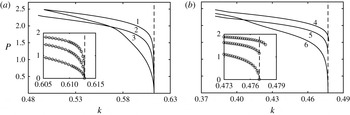
Bifurcation of
 $\unicode[STIX]{x1D719}_{p}$
for
 $(\unicode[STIX]{x1D6FF},\unicode[STIX]{x1D6E5})=(0,0)$
with respect to the domain wavenumber with (a)
 $\unicode[STIX]{x1D6F7}=0.1$
and (b)
 $\unicode[STIX]{x1D6F7}=0.3$
. The solution branches are measured by
 $P=(\max (\unicode[STIX]{x1D719}_{p})-\min (\unicode[STIX]{x1D719}_{p}))/\unicode[STIX]{x1D6F7}$
, and the excitation frequencies corresponding to the curves, as numbered in the panels, are
 $\unicode[STIX]{x1D6FA}_{1}=1.41\times 10^{-5}$
,
 $\unicode[STIX]{x1D6FA}_{2}=3.53\times 10^{-5}$
,
 $\unicode[STIX]{x1D6FA}_{3}=3.53\times 10^{-4}$
,
 $\unicode[STIX]{x1D6FA}_{4}=1.2\times 10^{-4}$
,
 $\unicode[STIX]{x1D6FA}_{5}=3\times 10^{-4}$
and
 $\unicode[STIX]{x1D6FA}_{6}=1.2\times 10^{-3}$
. Insets present local behaviour of the points (circles) found numerically near
 $k_{c}$
(vertical dashed lines).

In this subsection, we characterize branches of the case (i) periodic flows
 $\unicode[STIX]{x1D719}_{p}(\unicode[STIX]{x1D709},\unicode[STIX]{x1D70F})$
using the metric
 $P=(\max (\unicode[STIX]{x1D719}_{p})-\min (\unicode[STIX]{x1D719}_{p}))/\unicode[STIX]{x1D6F7}$
. Here, the maximum and minimum values of
 $\unicode[STIX]{x1D719}_{p}(\unicode[STIX]{x1D709},\unicode[STIX]{x1D70F}_{p})$
are taken at independent values of
 $f\unicode[STIX]{x1D70F}_{p}$
and
 $\unicode[STIX]{x1D709}$
during the excitation period. By scaling the difference by the mean thickness
 $\unicode[STIX]{x1D6F7}$
,
 $P$
is a suitable metric for comparing effects of
 $k$
,
 $\unicode[STIX]{x1D6FA}$
, and
 $\unicode[STIX]{x1D6F7}$
on the maximum variation of
 $\unicode[STIX]{x1D719}_{p}$
.
In figure 12, flow branches are tracked by continuation with respect to the fundamental wavenumber of the domain
 $k$
via the metric
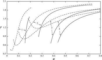
 $P$
for different values of
 $\unicode[STIX]{x1D6FA}$
. In panel (a), the mean film thickness is
 $\unicode[STIX]{x1D6F7}=0.1$
and curves 1, 2 and 3 are determined with
 $\unicode[STIX]{x1D6FA}=1.41\times 10^{-5}$
,
 $7.06\times 10^{-5}$
and
 $3.53\times 10^{-4}$
which are
 $0.4\unicode[STIX]{x1D6FC}_{m}$
,
 $2\unicode[STIX]{x1D6FC}_{m}$
,
 $10\unicode[STIX]{x1D6FC}_{m}$
, respectively. Generally,
 $P$
increases with distance from the cutoff wavelength
 $k_{c}=0.613$
, for each frequency sufficiently close to
 $k_{c}$
, and continued decrease of
 $k$
causes the film to rupture. It is also noteworthy that
 $P$
for curve 3, representing the largest frequency, overtakes that for curves 1 and 2 at sufficiently small values of
 $k$
, due to the effects just discussed for figure 11. Inspection of the inset in panel (a), with the data points for
 $P$
decreasing to zero as
 $k$
approaches
 $k_{c}$
, suggests supercritical bifurcation for each frequency. On the other hand, the existence of saddle nodes at which the bifurcation transitions from super to subcritical is suggested by panel (b). Here, with
 $\unicode[STIX]{x1D6F7}=0.3$
, flow branches with similar values of
 $P$
are obtained by increasing
 $\unicode[STIX]{x1D6FA}$
by an order of magnitude, in order to account for the larger values of
 $\unicode[STIX]{x1D6FC}$
associated with larger values of
 $\unicode[STIX]{x1D6F7}$
. Whereas here the largest frequency branch again exhibits supercritical branching, the lower frequency branches exhibit subcritical bifurcation, that is, stable deflected flows
 $\unicode[STIX]{x1D719}_{p}$
(and finite
 $P$
) are obtained at
 $k\geqslant k_{c}$
. We note that the subcritical branch is recovered as described in the next paragraph.
Further insight into the nature of the bifurcation and flow branches at criticality is presented in figure 13, where branches are tracked by continuation with respect to
 $\unicode[STIX]{x1D6F7}$
at
 $k=k_{c}(\unicode[STIX]{x1D6F7})$
. The solid lines depict branches obtained by first initializing a solution from a slightly perturbed profile in the linearly unstable regime, say
 $k=0.99k_{c}$
, and then using the resulting saturated profile as the initial condition for a computation at
 $k=k_{c}$
. Thus, the solid lines depict values of
 $\unicode[STIX]{x1D6F7}$
that bifurcate subcritically at the linear stability threshold as seen for curves 4 and 5 in figure 12(b). Although we expect these curves to decrease to
 $P=0$
at sufficiently low value of
 $\unicode[STIX]{x1D6F7}$
, indicating a saddle node at
 $\unicode[STIX]{x1D6F7}_{s}$
, numerical convergence is extremely slow in this vicinity because the growth rates of subcritical flows near
 $\unicode[STIX]{x1D6F7}_{s}$
decrease substantially. The lower edge of each curve has therefore been extended values of (
 $\unicode[STIX]{x1D6F7}$
,
 $P$
) that are low enough to speculate the proximity of
 $\unicode[STIX]{x1D6F7}_{s}$
. At sufficiently lower values of
 $\unicode[STIX]{x1D6F7}$
, the deflected solutions that are obtained in the linearly unstable regime decay quickly to the flat state at
 $k=k_{c}$
, indicative of supercritical bifurcation.
The upper bound of each solid curve in figure 13 has been continued until rupture. That is, as
 $\unicode[STIX]{x1D6F7}$
is increased for fixed
 $\unicode[STIX]{x1D6FA}$
, the film growth rates become much larger than growth induced by the excitation, and rupture occurs when the destabilization period is too high. It is therefore worth noting in figure 13 that the range of
 $\unicode[STIX]{x1D6F7}$
for which subcritical solutions exist decreases with
 $\unicode[STIX]{x1D6FA}$
. Following this trend, it may be reasonable to expect subcritical bifurcation at
 $\unicode[STIX]{x1D6F7}=0.1$
, albeit for only a vanishingly narrow range of
 $\unicode[STIX]{x1D6FA}$
.
Flow branches for case (i) near the linear stability threshold
 $k=k_{c}$
as a function of the mean initial film thickness
 $\unicode[STIX]{x1D6F7}$
. The excitation frequencies for the curves labelled 1–4 are:
 $\unicode[STIX]{x1D6FA}_{1}=3.3\times 10^{-5}$
,
 $\unicode[STIX]{x1D6FA}_{2}=1\times 10^{-4}$
,
 $\unicode[STIX]{x1D6FA}_{3}=1\times 10^{-3}$
and
 $\unicode[STIX]{x1D6FA}_{4}=3.3\times 10^{-3}$
. Solid and dashed curves represent separate branches obtained for each frequency.

Finally, a hint of further complexity to the bifurcation structure is provided by the dashed curves in figure 13, which characterize solutions uniquely different from those of the ‘lower’ branch, despite being calculated by the same frequencies. Notably, these ‘upper’ branches extend to much lower values of
 $\unicode[STIX]{x1D6F7}$
than the ‘lower’ branches and, similarly, represent different branches when extended to values of
 $k<k_{c}$
. It is emphasized that the basins of attraction of the regimes representing the upper branches are much narrower than those for the regimes on the lower branches.
4.6 Long-domain flows
Whereas only interfacial profiles characterized by a single major crest have been considered above, here we will focus on the dynamical features that emerge when the periodic domain is large enough to contain multiple major crests. The possibility of such profiles of the film interface stems from the linear theory: consider normal perturbations to (2.17) with the form
 $\unicode[STIX]{x1D719}=\unicode[STIX]{x1D6F7}+\hat{\unicode[STIX]{x1D719}}(\unicode[STIX]{x1D70F})\exp (\text{i}nk\unicode[STIX]{x1D709})$
, with positive integer
 $n$
, which leads to a time-averaged linear growth rate of
 $$\begin{eqnarray}\displaystyle \unicode[STIX]{x1D6FC}_{n}=-(nk)^{4}\unicode[STIX]{x1D6F7}^{3}+\left(\frac{\unicode[STIX]{x1D6FF}\unicode[STIX]{x1D6E5}}{(1+\unicode[STIX]{x1D6F7})^{2}}\unicode[STIX]{x1D6F7}^{2}+\frac{1+2\unicode[STIX]{x1D6E5}^{2}}{2(1+\unicode[STIX]{x1D6F7})^{3}}\unicode[STIX]{x1D6F7}^{3}\right)(nk)^{2} & & \displaystyle\end{eqnarray}$$
and a cutoff wavenumber for the
 $n$
th mode
 $k_{cn}=k_{c}/n$
. The growth rates
 $\unicode[STIX]{x1D6FC}_{n}$
, depicted for case (i) in figure 14 with
 $n=1$
, 2, 3 and 4, demonstrate that a single linearly unstable wavenumber, i.e. the fundamental harmonic
 $k$
, is excited only when
 $k_{c}/2<k<k_{c}$
. As the fundamental domain wavenumber is decreased, higher harmonic perturbations become unstable at each
 $k_{cn}$
, starting with the second harmonic at
 $k=k_{c2}$
. In general, the amplification of multiple perturbation wavenumbers within these ‘long domains’ drives nonlinear behaviour absent from short domains, such as pattern replication and wave coarsening. In principle, the influence of
 $\unicode[STIX]{x1D6FA}$
mirrors that discussed for short domains, i.e. long-time stable solutions to (2.17) are found for values of
 $\unicode[STIX]{x1D6FA}$
commensurate with
 $\unicode[STIX]{x1D6FC}_{n}$
. However, because long domains are characterized by multiple positive values of
 $\unicode[STIX]{x1D6FC}_{n}$
, we expect the bifurcation structure and solution branches to be significantly more complex than for short domains. Detailed numerical investigations of long-domain dynamics of nonlinear wave equations have been given by Smyrlis & Papageorgiou (Reference Smyrlis and Papageorgiou1991) for the Kuramoto–Sivashinsky equation and by Thiele & Knobloch (Reference Thiele and Knobloch2004) for a thin liquid film on an inclined isothermal wall. Such detail, however, is beyond the scope of this work and we instead report on qualitative behaviours inherent to long domains.
Case (i) perturbation growth rates for domain harmonics
 $nk$
with
 $n=1$
, 2, 3 and 4. Inset focuses on a range of domain wavenumbers within which both the
 $2k$
and
 $k$
harmonics are unstable, and the dashed vertical lines highlight values of
 $k$
used to calculate the results in figures 15–19.

As will be seen, in some cases the description of ‘saturated’ that applied to the short-domain flows
 $\unicode[STIX]{x1D719}_{p}$
must be modified for long-domain flows. Furthermore, the transient dynamics associated with growth from an initial condition depends significantly on the form of the condition. In order to minimize bias and encourage quick saturation, long-domain computations are initialized with a perturbation composed of random amplitudes and phases of the first six domain spatial harmonics. As a result, we find that repeated computations exhibit unique initial transients that may include coarsening and replicating events, however, for the cases we present, the saturated flows are independent of these transients.
Temporally periodic film profiles for case (i) with
 $\unicode[STIX]{x1D6FA}=3.528\times 10^{-5}$
and wavenumber
 $k$
set to (a) 0.2574 and (b) 0.2512. Solid and dashed lines correspond to profiles obtained at
 $f\unicode[STIX]{x1D70F}_{p}=0$
and
 $0.5$
, respectively.

The following discussion pertains to time-periodic flows
 $\unicode[STIX]{x1D719}_{p}$
of (2.17) obtained on long domains where both the
 $k$
and
 $2k$
perturbations are unstable and
 $\unicode[STIX]{x1D6FA}=3.528\times 10^{-5}$
. Whereas single crested profiles (that often rupture) are obtained when the domain wavenumber is close to
 $k_{c2}$
, where
 $\unicode[STIX]{x1D6FC}_{1}>\unicode[STIX]{x1D6FC}_{2}$
, time-periodic profiles containing multiple major crests are obtained for longer domains, in particular, where
 $\unicode[STIX]{x1D6FC}_{2}>\unicode[STIX]{x1D6FC}_{1}$
, as depicted in both panels of figure 15. Here, both profiles exhibit temporal periodicity satisfying the designation
 $\unicode[STIX]{x1D719}_{p}$
as used in the previous short-domain results. In panel (a), where
 $k=0.2574$
, Fourier analysis confirms that the interfacial profile is replicated, of 2
 $k$
spatial periodicity, because the amplitudes of all odd numbered spatial harmonics (wavenumbers
 $k$
,
 $3k$
, etc.) have decayed to zero. In panel (b), where
 $k=0.2512$
and the relative magnitude of
 $\unicode[STIX]{x1D6FC}_{2}$
to
 $\unicode[STIX]{x1D6FC}_{1}$
has increased, the flow saturates to
 $\unicode[STIX]{x1D719}_{p}$
which contains odd harmonics and bears
 $k$
spatial periodicity. Comparison of the lateral positions of the peaks, at both
 $f\unicode[STIX]{x1D70F}_{p}=0$
and 0.5, reveals that the peak locations oscillate laterally throughout the excitation, in opposite directions. In contrast, the lateral peak locations remain fixed for the replicated flow in panel (a) as well as short-domain flows of the previous sections.
Time series of the local film thickness
 $\unicode[STIX]{x1D719}_{q}(\unicode[STIX]{x1D709}=0)$
, for case (i) with
 $\unicode[STIX]{x1D6FA}=3.528\times 10^{-5}$
and wavenumber
 $k=0.2482$
. The series begins at a time
 $f\unicode[STIX]{x1D70F}_{q}=0$
that corresponds to a time
 $f\unicode[STIX]{x1D70F}$
where
 $\cos \unicode[STIX]{x1D6FA}\unicode[STIX]{x1D70F}=1$
and the initial transients have decayed.

4.7 Quasiperiodic flow
Not all saturated flows on long periodic domains satisfy
 $\unicode[STIX]{x1D719}_{p}(\unicode[STIX]{x1D709},f\unicode[STIX]{x1D70F})=\unicode[STIX]{x1D719}_{p}(\unicode[STIX]{x1D709},(n/2)f\unicode[STIX]{x1D70F})$
and therefore can not be classified as periodic flows. For example, this requirement is clearly not satisfied by the time series of
 $\unicode[STIX]{x1D719}(\unicode[STIX]{x1D709}=0)$
obtained at 0.2482, as depicted in figure 16 for 100 excitation periods. Nevertheless, this flow still exhibits saturation in the sense that time series of the spatial harmonic amplitudes enter steady limit cycles. To discuss such quasiperiodic flows
 $\unicode[STIX]{x1D719}_{q}$
, as in figure 16, we utilize the time coordinate
 $f\unicode[STIX]{x1D70F}_{q}$
where
 $f\unicode[STIX]{x1D70F}_{q}=0$
corresponds to a time
 $f\unicode[STIX]{x1D70F}$
at which
 $\cos \unicode[STIX]{x1D6FA}\unicode[STIX]{x1D70F}=1$
and saturation has occurred. While the series in figure 16 appears to repeat itself approximately every 45 periods, the insets highlight subtle differences in the oscillations of the thickness
 $\unicode[STIX]{x1D719}$
at times separated by the apparent repetition period.
Film profiles obtained throughout an excitation period associated with the time series presented in figure 16. The 12 solid line profiles depicted in panels (a–d) correspond to times ranging from
 $24f\unicode[STIX]{x1D70F}_{q}=0$
to 11 as in figure 8 and the arrows denote the direction of increasing time. The dashed profile in panel (d) represents the interfacial shape at
 $24f\unicode[STIX]{x1D70F}_{q}=12$
.

Translated film profiles obtained at times for which
 $\cos \unicode[STIX]{x1D6FA}\unicode[STIX]{x1D70F}_{q}=1$
, from the time series presented in figure 16. The translation is emphasized by presenting profiles separated by two excitation periods. The translation speed, as a function of the wavenumber, is presented in the inset for
 $\unicode[STIX]{x1D6FA}=2.822\times 10^{-5}$
(solid line),
 $3.175\times 10^{-5}$
(dashed) and
 $3.528\times 10^{-5}$
(dash-dotted).

Time series of the (a) local film thickness
 $\unicode[STIX]{x1D719}$
, located at
 $\unicode[STIX]{x1D709}=0$
and (b) profile translation speed for case (i) with
 $\unicode[STIX]{x1D6FA}=3.528\times 10^{-5}$
and wavenumber
 $k=0.2463$
.

The spatial character of the quasiperiodic time series in figure 16 is resolved by considering the corresponding profiles
 $\unicode[STIX]{x1D719}_{q}(\unicode[STIX]{x1D709},f\unicode[STIX]{x1D70F}_{q})$
, which are depicted in figure 17 for times
 $0\leqslant f\unicode[STIX]{x1D70F}_{q}\leqslant 1/2$
. The first novel feature that can be observed is that the major peak amplitudes have become rather disparate, in contrast to figure 15, where these amplitudes are either approximately or exactly equal. Second, while the peaks exhibit the lateral oscillations seen in figure 15(b), the dashed profile in figure 17(d), at
 $24f\unicode[STIX]{x1D70F}_{q}=12$
, has shifted slightly to the right of the
 $f\unicode[STIX]{x1D70F}_{q}=0$
profile in panel (a). The film exhibits a mean translation to the right over the course of an excitation period. The dashed profile in panel (d) of figure 17, corresponding to
 $f\unicode[STIX]{x1D70F}_{q}=1$
, has shifted slightly to the right of the
 $f\unicode[STIX]{x1D70F}_{q}=0$
profile in panel (a).
The profiles depicted in figure 18, which are sampled at times where
 $\cos \unicode[STIX]{x1D6FA}\unicode[STIX]{x1D70F}_{q}=1$
and intervals of two excitation periods, emphasize that the film profile is translating to the right. To investigate this translation, the positions of the spatial harmonics are determined by Fourier analysis, and then a rate of translation
 $c$
is calculated as the change in position per excitation period. When sampled at the excitation frequency, at times when
 $\cos \unicode[STIX]{x1D6FA}\unicode[STIX]{x1D70F}_{q}=1$
, we find that all spatial harmonics translate at the same rate
 $c=0.559$
. Taking into account the domain wavelength
 $\unicode[STIX]{x1D706}=25.31$
, the profile is expected to translate across a single domain wavelength every 45.29 periods.
The quasiperiodicity observed in the time series in figure 16 therefore resembles the superposition of a travelling frequency and the excitation frequency. The emergence of travelling wave flows from (2.17) is rather striking, because it contains no terms traditionally associated with advection. Rather, we suspect that the disparity in the two major crest thicknesses contributes to effective lateral thermal gradients within the domain, which, when averaged over the excitation and the accompanying thickness oscillations, result in a mean thermocapillary stress and profile drift. Furthermore, using randomized initial conditions, we find these flows may travel either to the left or the right, at speeds of the same magnitude.
The inset of figure 18 depicts the translation rates
 $c$
of such flows over ranges
 $k$
for three different excitation frequencies
 $\unicode[STIX]{x1D6FA}=2.822\times 10^{-5}$
,
 $3.175\times 10^{-5}$
and
 $3.528\times 10^{-5}$
. For each frequency,
 $c$
decays to zero once
 $k$
is set slightly higher than the upper edge of the branch, and the resulting periodic flow
 $\unicode[STIX]{x1D719}_{p}$
resembles the profiles depicted in figure 15(b). Then, for
 $k$
set slightly lower than the lower edge of the branch, flows with
 $\unicode[STIX]{x1D6FA}=2.822\times 10^{-5}$
and
 $3.175\times 10^{-5}$
lose stability to rupturing flows characterized by one major crest.
As depicted in figure 19, more nuance is encountered with the time series
 $\unicode[STIX]{x1D719}_{q}$
for
 $\unicode[STIX]{x1D6FA}=3.528\times 10^{-5}$
, where
 $k=0.2463$
is situated slightly below the lower edge of the corresponding branch in inset of figure 18. Here, the time series
 $\unicode[STIX]{x1D719}_{q}$
in panel (a) of figure 19 displays a travelling flow reminiscent of figures 16–18. This series
 $\unicode[STIX]{x1D719}_{q}$
however displays a temporal oscillation with a period even longer than the travelling period, of approximately 400 excitation periods. In contrast to the travelling flows investigated in the inset of figure 18, where
 $c$
is constant, figure 19(b) shows that
 $c$
contains both major and minor oscillations.
5 Potential experimental settings
We will now use the model to predict behaviour of self-rewetting films in potential experimental settings, with initial intent to determine the conditions at which one may observe the periodic flow in figures 7–9 where
 $(\unicode[STIX]{x1D6E5},\unicode[STIX]{x1D6FF},\unicode[STIX]{x1D6F7},k,\unicode[STIX]{x1D6FA})=$
(0, 0, 0.1, 0.55,
 $7.06\times 10^{-5}$
). Specifically, we consider films of a 0.7 molar aqueous solution of butanol, for which (Savino et al.
Reference Savino, Cecere, VanVaerenbergh, Abe, Pizzirusso, Tzevelecos, Mojahed and Galand2013) have reported the surface tension as a function of temperature. Analysing their data, we find
 $\unicode[STIX]{x1D703}_{0}=66.3\,^{\circ }$
C,
 $\unicode[STIX]{x1D70E}_{0}=0.0263~\text{N}~\text{m}^{-1}$
and
 $\unicode[STIX]{x1D6FE}=2.98\times 10^{-6}~\text{N}~\text{m}^{-1}$
K
 $^{-2}$
. The viscosity and thermal conductivity of the dilute mixture are set equal to that of water,
 $\unicode[STIX]{x1D707}=4.3\times 10^{-4}~\text{Pa}~\text{s}$
and
 $\unicode[STIX]{x1D705}=0.66~\text{W}~\text{m}^{-1}~\text{K}^{-1}$
.
The temperature differences
 $\unicode[STIX]{x1D6E5}$
and
 $\unicode[STIX]{x1D6FF}$
remain defined as in (2.9), and, for this case where
 $\unicode[STIX]{x1D6E5}=\unicode[STIX]{x1D6FF}=0$
,
 $\unicode[STIX]{x1D703}_{s}$
and
 $\bar{\unicode[STIX]{x1D703}}_{g}$
will both be set to
 $\unicode[STIX]{x1D703}_{0}$
. Via (2.16), (2.9) and (2.6), the remaining dimensionless parameters are defined as
 $$\begin{eqnarray}\displaystyle \unicode[STIX]{x1D6F7}=\frac{q}{\unicode[STIX]{x1D705}}h_{0},\quad k=\frac{\unicode[STIX]{x1D705}}{q}\left(\frac{\unicode[STIX]{x1D70E}_{0}}{\unicode[STIX]{x1D6FE}\hat{\unicode[STIX]{x1D703}}_{g}^{2}}\right)^{1/2}k^{\ast },\quad \unicode[STIX]{x1D6FA}=\unicode[STIX]{x1D714}\frac{\unicode[STIX]{x1D705}}{q}\frac{\unicode[STIX]{x1D70E}_{0}\unicode[STIX]{x1D707}}{(\unicode[STIX]{x1D6FE}\hat{\unicode[STIX]{x1D703}}_{g}^{2})^{2}}, & & \displaystyle\end{eqnarray}$$
where
 $k^{\ast }$
is the dimensional wavenumber, and provide freedom to set all but three parameters of the dimensional system. Although, in an experiment, one is far more likely to have control of
 $h_{0}$
,
 $\unicode[STIX]{x1D714}$
, and
 $\hat{\unicode[STIX]{x1D703}}_{g}$
, with
 $k^{\ast }$
as an output, we will fix
 $\hat{\unicode[STIX]{x1D703}}_{g}$
 $a$
 $priori$
because the relations for
 $\unicode[STIX]{x1D6F7}$
,
 $k$
and
 $\unicode[STIX]{x1D6FA}$
in (5.1a–c
) are linear in
 $h_{0}$
,
 $k^{\ast }$
and
 $\unicode[STIX]{x1D714}$
. We therefore set
 $\hat{\unicode[STIX]{x1D703}}_{g}=6\,^{\circ }$
C, a thermal excitation characteristic of a high power acoustic wave in air at standard temperature and pressure.
Of greatest uncertainty is prescription of
 $q$
, the rate at which heat is exchanged between the liquid and gas phases at the film interface. Several thin film works, such as Kalliadasis, Kiyashko & Demekhin (Reference Kalliadasis, Kiyashko and Demekhin2003) and Nepomnyashchy, Velarde & Colinet (Reference Nepomnyashchy, Velarde and Colinet2001), state that
 $q$
, or, likewise, the Biot number, is often unknown and therefore models can be used to make qualitative predictions at best. To proceed with a representative value for
 $q$
, we observe that Holman (Reference Holman2010) has provided approximate values for free convection heat transfer that range in the interval 4.5–
 $890~\text{W}\,\text{m}^{-2}\,\text{K}^{-1}$
. Additionally, Kalliadasis et al. (Reference Kalliadasis, Ruyer-Quil, Scheid and Velarde2012) have discussed the relevance of thin film heat transfer coefficients ranging from 100–
 $500~\text{W}\,\text{m}^{-2}\,\text{K}^{-1}$
. Conceivably, one also could determine
 $q$
experimentally by measuring the instability wavelength at criticality for a given threshold value of
 $\hat{\unicode[STIX]{x1D703}}_{g}$
, see (3.5).
Moving forward, with
 $q=100~\text{W}\,\text{m}^{-2}\,\text{K}^{-1}$
, we use (5.1a–c
) to determine the set of conditions (
 $\unicode[STIX]{x1D703}_{s}$
,
 $\bar{\unicode[STIX]{x1D703}}_{g}$
,
 $h_{0}$
,
 $\unicode[STIX]{x1D706}^{\ast }$
,
 $f^{\ast }$
)
 $=$
(
 $66.3\,^{\circ }$
C,
 $66.3\,^{\circ }$
C, 0.66 mm, 1.18 m,
 $1.73\times 10^{-6}$
Hz) at which the dimensionless dynamics presented in figures 7–9 is applicable to films of aqueous butanol. Here,
 $\unicode[STIX]{x1D706}^{\ast }$
and
 $f^{\ast }$
are the dimensional wavelength and ordinary frequency, respectively. Although the film thickness is experimentally reasonable, the wavelength, and even more so, the frequency, are not. Conceivably one could increase
 $h_{0}$
, so that larger values of
 $\unicode[STIX]{x1D6F7}$
, and, accordingly, larger values of
 $\unicode[STIX]{x1D6FA}$
are relevant, however, continued increase in
 $h_{0}$
will render invalid the assumption that buoyancy is negligible. Furthermore, the wavelength is independent of
 $h_{0}$
.
Instead, it appears that introduction of substrate heating/cooling and bias, by considering finite
 $\unicode[STIX]{x1D6E5}$
and
 $\unicode[STIX]{x1D6FF}$
, is the most practical means by which non-rupturing flows can be generated in experimental settings. By doing so, the growth rates and wavenumbers can be increased significantly. For example, with
 $\unicode[STIX]{x1D6E5}=2$
and
 $\unicode[STIX]{x1D6FF}=1$
, we find via (3.5) that
 $k_{c}=4.46$
and
 $\unicode[STIX]{x1D6FC}_{m}=0.0991$
. We then find that the evolution equation generates a non-rupturing flow for the parameters (
 $\unicode[STIX]{x1D6E5}$
,
 $\unicode[STIX]{x1D6FF}$
,
 $\unicode[STIX]{x1D6F7}$
,
 $k$
,
 $\unicode[STIX]{x1D6FA}$
)
 $=$
(2, 1, 0.1, 4.3, 0.0991). We note that the resulting periodic flow strongly resembles that presented in figure 9, with the exception that destabilization cells are more tightly constrained to the vicinity of the major film trough. For aqueous butanol with an excitation amplitude of
 $\hat{\unicode[STIX]{x1D703}}_{g}=6^{\circ }$
C, the corresponding dimensional parameters are (
 $\unicode[STIX]{x1D703}_{s}$
,
 $\bar{\unicode[STIX]{x1D703}}_{g}$
,
 $h$
,
 $\unicode[STIX]{x1D706}^{\ast }$
,
 $f^{\ast }$
)
 $=$
(
 $72.3\,^{\circ }$
C,
 $84.3\,^{\circ }$
C, 0.66 mm, 0.151 m, 0.00244 Hz), which are much more feasible. Here, the wavelength remains large. Inspection of (5.1a–c
) reveals that the wavelength can be decreased by increasing the excitation amplitude, however, one must bear in mind that the range of applicable dimensional temperatures is bounded by phase transitions at which model assumptions will lose validity. For example, with
 $\unicode[STIX]{x1D6E5}=2$
and
 $\unicode[STIX]{x1D6FF}=1$
, an increase of
 $\hat{\unicode[STIX]{x1D703}}_{g}$
to
 $10\,^{\circ }$
C corresponds to
 $\unicode[STIX]{x1D703}_{s}=76.3\,^{\circ }$
C and
 $\bar{\unicode[STIX]{x1D703}}_{g}=96.3\,^{\circ }$
C. Hence, the gas temperature will rise above the saturation temperature of pure water (at atmospheric pressure) during the warm cycle of the excitation and phase change processes will become important.
A different choice of an operating fluid can shift the value of
 $\unicode[STIX]{x1D703}_{0}$
and increase the range of applicable temperatures. For example, using data reported by Legros (Reference Legros1986), we find for aqueous heptanol that
 $\unicode[STIX]{x1D703}_{0}=40.7\,^{\circ }$
C,
 $\unicode[STIX]{x1D70E}_{0}=0.0375~\text{N}~\text{m}^{-1}$
and
 $\unicode[STIX]{x1D6FE}=3.42\times 10^{-6}~\text{N}~\text{m}^{-1}~\text{K}^{-2}$
. Using these values, and increasing of the excitation amplitude to
 $\hat{\unicode[STIX]{x1D703}}_{g}=15^{\circ }$
, the dimensionless parameters (
 $\unicode[STIX]{x1D6E5}$
,
 $\unicode[STIX]{x1D6FF}$
,
 $\unicode[STIX]{x1D6F7}$
,
 $k$
,
 $\unicode[STIX]{x1D6FA}$
)
 $=$
(2, 1, 0.1, 4.3, 0.496) correspond to dimensional values of (
 $\unicode[STIX]{x1D703}_{s}$
,
 $\bar{\unicode[STIX]{x1D703}}_{g}$
,
 $h_{0}$
,
 $\unicode[STIX]{x1D706}^{\ast }$
,
 $f^{\ast }$
)
 $=$
(
 $55.7\,^{\circ }$
C,
 $85.7\,^{\circ }$
C, 0.66 mm, 0.0673 m, 0.0175 Hz). Here, the wavelength is measurable, and the mean gas temperature is low enough such that the effects of phase change are mitigated. Here we have considered substrate cooling as a means to drive instability and increase the growth rates, however, substrate heating could also be used if one were to operate at temperatures lower than
 $\unicode[STIX]{x1D703}_{0}$
. In such situations, the operating temperature range could then be expanded by choosing shorter carbon-chained alcohols, which are characterized by larger values of
 $\unicode[STIX]{x1D703}_{0}$
.
6 Conclusion
To summarize, in this work we have developed and investigated a model that describes the interaction of an oscillatory gas temperature with a liquid film whose surface tension depends nonlinearly on temperature. Although this work was inspired by fluids that exhibit a surface tension minimum with respect to temperature, the model also applies to any fluid whose surface tension shows local nonlinear dependence on temperature. That is, for small variations in temperature, the surface tension of the fluid as a function of temperature will contain terms that are linear and quadratic in temperature, (2.4) would be valid in the vicinity of the nonlinearity, and (2.17) would apply. The main consequence is that thermal excitation in this vicinity generates a time-averaged driving force for film instability when the temperature of film–substrate interface is held fixed. Thus our finding is distinguished from previous works on thermal excitations by Or & Kelly (Reference Or and Kelly2002) and Smorodin et al. (Reference Smorodin, Mikishev, Nepomnyashchy and Myznikova2009), who found that films with linear surface tension are destabilized only when heat fluxes are prescribed through the substrate. Perhaps the most interesting aspect of the model is the emergence of time-periodic, non-rupturing flows on periodic domains when the excitation frequency is tuned approximately to the linear growth rate. A rich set of nonlinear dynamical features was subsequently presented, for the case where the film lies on a substrate that is fixed to the mean gas temperature and the temperature corresponding to the minimum surface tension. These features include the role of the excitation frequency, super- and subcritical bifurcation, and transitions to travelling flows.
The conditions at which experimental flows will resemble those predicted by (2.17) are not immediately clear. In fact, quantitative prediction of experimental thermocapillary phenomena is fleeting due to uncertainty in the liquid–gas heat transfer rate. Upon estimating the heat transfer rate, we found that the excitation frequencies corresponding to non-rupturing flows are generally small, for the case where the substrate and mean gas temperatures are fixed to that which gives the minimum surface tension. Our model nevertheless predicts that larger, experimentally relevant frequencies will drive film rupture in this situation. One must bear in mind however that our model assumptions break down for excessively large frequencies. The experimental feasibility of generating saturated flows was then found to increase considerably when the thermal excitation is augmented with substrate heating/cooling. Towards expanding the relevant dimensional parameter space, it may also be of interest to consider different thermal boundary conditions, such as constant flux at the film–substrate interface, as well as applying the thermal excitation from the substrate.
Acknowledgements
The research was partially supported by the grant no. 345/13 to A.O. and Y.A. from the Israel Science Foundation. W.B. was supported in part at the Technion by an Aly Kaufman Fellowship. A.O. acknowledges support by D. T. Siegel, Chair of Fluid Mechanics.