2.2 Definitions and formulations

The concept of a CSP is fundamental in constraint programming. Hence, we need to give a formal definition of it. We first introduce the concepts of a variable domain and constraint, and then define the concept of a CSP and related concepts. Then we present different formulations for the same problem to show that a CSP can be modeled in many different ways. One of the most important tasks for solving a real-life problem is to represent the problem as a CSP, that is, in terms of variables, domains, and constraints.

2.2.2 Formulations of a constraint satisfaction problem

Solving a CSP must be carried out in two different phases:

• • Modeling the problem as a constraint satisfaction problem. In this phase, the problem is modeled by means of a CSP syntaxis, that is, by a set of variables, domains, and constraints.

• • Solving the resultant constraint satisfaction problem. Once the problem is modeled as a CSP, there exist many constraint satisfaction techniques to solve it.

Generally, a problem can be formulated in many different ways, even in natural language. For each problem, the representation of a potential solution and its corresponding interpretation implies the search space and its size. This is an important point to recognize: ‘The size of the search space is not determined by the problem; it’s determined by your representation and the manner in which you handle this encoding’ (Michalewicz & Fogel, Reference Michalewicz and Fogel2000). In the following text, we present some classical examples (Van Hentenryck, Reference van Hentenryck1989; Ruttkay, Reference Ruttkay1998; Bistarelli, Reference Bistarelli2004) which can be modeled in two different ways. We can observe the advantage of an appropriate model to be solved more efficiently.

A crypto-arithmetic puzzle

We consider the classical ‘crypto-arithmetic’ puzzle: SEND + MORE = MONEY. The variables {s, e, n, d, m, o, r, y} represent digits between 0 and 9 and the task is finding values for them such that the following arithmetic operation is correct:

Though it is not stated in the rules directly, it is implied that zero cannot be the first digit in any of the three numbers. Thus, the unique solution of the problem is 9567 + 1085 = 10 652. The easier way to model the problem is by having a variable for every letter, where the variable stands for the digit associated with the letter ({0,…, 9}). The constraints are obvious from the problem specification taken into account that all variables must be assigned to different values. Thus, the constraints are:

• •

• • ;

This formulation of the problem is not very appropriate for many search algorithms such as simple Backtracking (BT)Footnote 1, due to the fact that all variables must be previously assigned to check these constraints. Thus, the search space cannot be pruned to improve the search process.

In the following text, we present a different model of the problem. This model decomposes each constraint into a set of constraints. We assume that zero cannot be the first digit in any of the three numbers so that m and s cannot be fixed to 0. Owing to the topology of the problem, m from money can only take value 0 or 1, but due to the former assumption that m must be fixed to one, the domain of s is reduced to {1,…,9}. This new model includes three additional variables c ₁, c ₂, c ₃. The domains of the variables are now:

• 

• 

• 

• 

and the above equation constraint can be decomposed to the following constraints:

• •

• •

• •

• •

• •

The second model has the advantage that the constraints are composed by a smaller number of variables than in the previous model, so that these constraints can be more efficiently checked during the BT search and thus inconsistencies can be found earlier.

The eight-queens problem

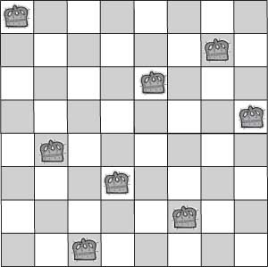
The second example is the popular eight-queens problem (Figure 1). The objective is to place eight queens on the chessboard such that they do not attack each other. In order to formulate this problem as a CSP, the location of the queens should be given by variables, and the fact that they do not attack each other must be modeled in terms of constraints.

Figure 1

Example of a constraint satisfaction problem (eight-queens)

One way to do this is to assign a variable to each queen. As the eight queens must be placed in eight different columns, we can identify each queen by its column, and represent its position by a variable, which indicates the row of the queen. The domain of each of the variables is the number of available rows. Thus, the domain of x ₁,…,x ₈ is 1, 2,…,8. For any two different variables the following two constraints must hold, expressing that the queens should be in different rows and on different diagonals:

• x_i ≠ x_j

• |x_i−x_j| ≠ |i−j|

In this formulation of the problem, we have to find a solution out of the total possible instantiations of the variables, whose number is 8⁸. This formulation, though it seems natural, does contain the following trick: a part of the requirements of the problem is reflected in the representation, not in the constraints. We could have used the most straightforward representation, namely identifying the squares of the chessboard by the numbers 1, 2,…,64, and having eight variables for each of the eight queens all with the domain {1, 2,…,64}. In this case, the ‘different columns’ requirement should also be expressed by constraints, and all the three types of constraints become more intrinsic to formulate (Ruttkay, Reference Ruttkay1998). The total number of possible arrangements becomes as large as 64,⁸ containing a configuration of queens multiple times due to the identification of the eight queens. Therefore, we have many reasons to prefer the first representation over the second one.

Different models may yield very different amount of time and space. Hence, when modeling a problem as a CSP, one has to pay attention to different possibilities, and try to commit to the one, which will be the easiest to cope with. The in-depth analysis of the different solution methods and of the characteristics of the CSPs may provide a basis to make a good choice. Several cases have been reported in which a notoriously difficult problem could be solved finally as a result of a change of its representation.

2.3 Consistency techniques

Consistency techniques were first introduced for improving the efficiency of picture recognition programs, by researchers in AI (Waltz, Reference Waltz1972). The number of possible combinations can be huge, while only very few are consistent. By eliminating redundant values from the problem definition, the size of the solution space decreases. Reduction of the problem can be done once, as a pre-processing step for another algorithm, or step by step, interwoven with the exploration of the solution space by a search algorithm. In the latter case, subsets of the solution space may be cut off, saving the search algorithm the effort of systematically investigating the eliminated elements, which otherwise would happen, even repeatedly. If, as a result of reduction, any domain becomes empty, then it is known immediately that the problem has no solution (Ruttkay, Reference Ruttkay1998).

Local inconsistencies are single values or a combination of values for variables that cannot participate in any solution because they do not satisfy some consistency property. For instance, if a value a of variable x is not compatible with all the values in a variable y that is constrained with x, then a is inconsistent and this value can be removed from the domain of the variable x.

One should be careful with not spending more effort on reduction than what will ‘pay off’ in the boosted performance of the search algorithm to be used to find a solution to the reduced problem. The reduction algorithms eliminate values by propagating constraints. The amount of constraint propagation is characterized by the consistency level of the problem; hence, these algorithms are also called consistency algorithms. The iterative process of achieving a level of consistency is sometimes referred to as the relaxation process, which should not be mixed up with relaxation of constraints.

Consistency techniques have a long tradition in CSP research. Below, we introduce the most well-known and widely used algorithms for binary CSPs (CSPs with unary and binary constraints).

• • A CSP is node-consistent if all the unary constraints hold for all the elements of the domains. The straightforward node-consistency algorithm (NC), which removes the redundant elements by checking the domains one after the other, has O(dn) time complexity, where d is the maximum size of domains and n is the number of variables. Thus, enforcing this consistency ensures that all values of the variable satisfy all the unary constraints on that variable.

• • A CSP is arc-consistent if for any pair of constrained variables x_i, x_j, for every value a in D_i there is at least one value b in D_j such that the assignments (x_i, a) and (x _j, b) satisfy the constraint between x_i and x_j. Any value in the domain D_i of variable x_i that is not arc-consistent can be removed from D_i since it cannot be part of any solution.

The Revise-Domain procedure given below eliminates those elements from the domain of a variable x_i for which a given binary constraint cannot be satisfied. (The given pseudo-programs are based on ones in Tsang (Reference Tsang1993)).

Revise-Domain, when applied to pair (x_i, x_j), deletes all the values from the domain of x_i that are not compatible with values from the domain of x_j. The domain of x_j will not be modified by this procedure. The boolean value reduced indicates whether a value is deleted or not. Running the Revise-Domain procedure for all the binary constraints may not be enough to assure that the reduced problem is arc-consistent. In fact, it may be necessary to run it more than once on some constraints. Below, we give a widely used arc-consistency algorithm, called AC-3:

This algorithm reconsiders all binary constraints over (x_k, x_i) if the Revise-Domain procedure has modified the domain of variable x_i. Thus, when AC-3 ends, no domain can be reduced further and thus the problem is arc-consistent.

Arc-consistency has become very important in CSP solving and is in the heart of many CP languages.

• • A CSP is path-consistent if, for every pair of values a and b for two variables x_i and x_j, such that the assignments of a to x_i and b to x_j satisfy the constraint between x_i and x_j, there exist a value for each variable along any path between x_i and x_j such that all constraints along the path are satisfied. When a path-consistent problem is also node-consistent and arc-consistent, then the problem is said to be strongly path-consistent.

Path-consistency is not widely used in CSP solving due to its high time and space complexity. However, it is an important consistency techniques for CSPs with special properties such as temporal CSPs (Dechter et al., Reference Dechter, Meiri and Pearl1991).

2.4 Search techniques

A CSP can be solved by systematically exploring the solution space by an uninformed search. The algorithms instantiate variables one after the other in such a way that the partial instantiation is always consistent. If this is not possible for a variable on turn, that is, all the possible values are in conflict with some earlier assignment, then BT takes place.

The simplest search scenario is when the order of variables as well as the order of values to be considered next is fixed, and if a dead end occurs, then the latest instantiation is reconsidered. In this uninformed search, a depth-first backtrack search algorithm (Bitner & Reingold, Reference Bitner and Reingold1975) is used. While the worst-case time complexity of backtrack search is exponential, several heuristics to reduce its average-case complexity have been proposed in the literature (Dechter & Pearl, Reference Dechter and Pearl1988). However, determining which algorithms are superior to others remains difficult. Theoretical analysis provides worst-case guarantees which often do not reflect average performance. For instance, a BT-based algorithm that incorporates features such as variable ordering heuristics will often in practice have substantially better performance than a simpler algorithm without this feature (Haralick & Elliot, Reference Haralick and Elliot1980), and yet the two share the same worst-case complexity. In addition, constraint propagation techniques such as consistency techniques (node consistency, arc-consistency, etc.), are very appropriate for solving CSPs more efficiently.

In the following text, we present some well-known systematic search algorithms as well as the main heuristics that improve BT-based algorithms (variable ordering and value ordering; Sadeh & Fox, Reference Sadeh and Fox2003). They play an important role in CSP solving and have drawn a lot of attention mainly in binary problems. More information can be found in (Barták, Reference Barták1998; Rossi et al., Reference Rossi, Van Beek and Walsh2006).

2.4.1 Complete search algorithms

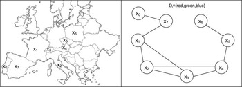
Most algorithms for solving CSPs search systematically through the possible assignments of values to variables. Such algorithms are guaranteed to find a solution, if one exists, or to prove that the problem is insoluble. The disadvantage of these algorithms is that they may take a very long time to do so. The actions of a search algorithm can be described by a search tree. We illustrate this with a toy example shown in Figure 2. The CSP in this figure is a small graph-coloring problem, in which the goal is to assign a color to each variable (country) such that connected variables (neighboring countries) do not share the same color.

Figure 2

Example of constraint satisfaction problem: a modified Europe coloring problem. The domain of each node (Country) is: {red, blue, green}. Adjacent nodes (Countries) must be assigned different colors

Generate-and-Test

The generate-and-test (GT) method originates from the naïve approach to solving combinatorial problems. First, the GT algorithm guesses the solution, and then it tests whether this solution is correct, that is, whether the solution satisfies the original constraints. In this paradigm, each possible combination of the variable assignments is systematically generated and tested to see if it satisfies all the constraints. The first combination that satisfies all the constraints is the solution. The number of combinations considered by this method is the size of the Cartesian product of all the variable domains.

Following the ordering (X ₀; X ₁; X ₂; X ₃; X ₄; X ₅; X ₆; X ₇) for the CSP described in Figure 2, the GT algorithm assigns values to all variables, for example, (X ₀ = red; X ₁ = blue; X ₂ = red; X ₃ = green; X ₄ = blue; X ₅ = red; X ₆ = green; X ₇ = red), and then it checks whether all constraints are satisfied.

The main disadvantage is that it is not very efficient because it generates many assignments of values to variables which are rejected in the testing phase. In addition, the generator leaves out the conflicting instantiations and generates other assignments independently of the conflict. Visibly, one can get far better efficiency if the validity of the constraint is tested as soon as its respective variables are instantiated. In fact, this method is used by the BT approach.

Backtracking Search

A simple algorithm for solving a CSP is BT search (Golomb & Baumert, Reference Golomb and Baumert1965; Bitner & Reingold, Reference Bitner and Reingold1975). BT works with an initially empty set of consistent instantiated variables and tries to extend the set to a new variable and a value for that variable. If successful, the process is repeated until all variables are included. If unsuccessful, another value for the most recently added variable is considered. Returning to an earlier variable in this way is called a backtrack. If that variable does not have any further values, then the variable is removed from the set, and the algorithm backtracks again. The simplest BT algorithm is called chronological BT because at a dead end the algorithm returns to the immediately earlier variable in the ordering.

The pseudo code of the basic BT Search (BT) algorithm is given:

Free variables are the variables that are not instantiated yet by the data structure instantiation. We initiate the Recursive BT procedure with free-variables = X, instantiation = ∅, and domains = D, where D are in the initial domains of the variables. When the procedure stops, it returns a consistent instantiation of all the variables in the structure solution, if the problem is solvable, and ∅ otherwise.

BT can be seen as a merge of the generate and test phases from the GT approach. In the BT method, variables are instantiated sequentially and as soon as all the variables relevant to a constraint are instantiated, the validity of the constraint is checked. If a partial solution violates any of the constraints, BT is performed to the most recently instantiated variable that still has alternatives available. Clearly, whenever a partial instantiation violates a constraint, BT is able to eliminate a subspace from the Cartesian product of all variable domains. Consequently, BT is strictly better than GT. However, its running time complexity for most non-trivial problems is still exponential.

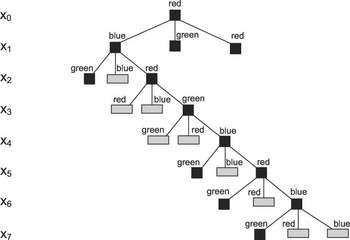
Figure 3 shows a part of the search tree expanded when BT processes the CSP described in Figure 2, using the ordering (X ₀; X ₁; X ₂; X ₃; X ₄; X ₅; X ₆; X ₇).

Figure 3

Part of the search tree explored by backtracking on the constraint satisfaction problem presented in Figure 2. Only a part of the search tree below X₀ = red and X₁ = blue is drawn. A black square denotes an instantiation from which further search can continue. A gray rectangle denotes a value that is not compatible with some previous value

There are three major drawbacks to the standard BT scheme. One is thrashing, that is, repeated failure due to the same reason. Thrashing occurs because the standard BT algorithm does not identify the real reason for the conflict, that is, the conflicting variables. Therefore, search in different parts of the space may keep failing for the same reason. Thrashing can be avoided by intelligent BT, that is, by a scheme in which BT is done directly to the variable that caused the failure. The other drawback of BT is having to perform redundant work. Even if the conflicting values of variables are identified during intelligent BT, they are not remembered for immediate detection of the same conflict in a subsequent computation. There is a BT-based method that eliminates both of the above drawbacks of BT. This method is traditionally called dependency-directed BT and is used in truth maintenance systems. It should be noted that using advanced techniques adds other expenses to the algorithm that has to be balanced with the overall advantage of using them. Finally, the basic BT algorithm still detects the conflict too late as it is not able to detect the conflict before it really occurs, that is, after assigning the values to all the variables of the conflicting constraint. This drawback can be avoided by applying consistency techniques to forward check the possible conflicts. We will analyze these techniques in the next section.

Look-Back Algorithms

BT can suffer from thrashing; the same dead end can be encountered many times. If X_i is a dead end, the algorithm will backtrack to X_{i− 1}. Suppose a new value for X_{i− 1} exists, but that there is no constraint between X_i and X_{i− 1}. The same dead end will be reached at X_i again and again until all values of X_{i− 1} have been explored.

Look-back algorithms try to exploit information from the problem to behave more efficiently in dead-end situations. Like BT, look-back algorithms perform consistency checks backward (between the current variable and past variables).

Backjumping (BJ; Gaschnig, Reference Gaschnig1979) is an algorithm similar to BT except that it behaves in a more intelligent manner when a dead end (X_i) is found. Instead of BT to the previous variable (X_{i− 1}), BJ backjumps to the deepest past variable X_j, j < i that is in conflict with the current variable X_i. It is said that variable X_j is in conflict with the current variable X_i if the instantiation of X_j precludes one of the values in X_i. Changing the instantiation of X_j may make it possible to find a consistent instantiation of the current variable. Thus, BJ avoids any redundant work that BT does by trying to reassign variables between X_j and the current variable X_i.

Conflict-directed BJ (Prosser, Reference Prosser1993), backmarking (Gaschnig, Reference Gaschnig1977), and learning (Frost & Dechter, Reference Frost and Dechter1994) are examples of look-back algorithms.

Look-Forward Algorithms

As we have explained, look-back algorithms try to enhance the performance of BT by more intelligent behavior when a dead end is found. Nevertheless, they still perform only backward consistency checks and ignore the future variables.

Look-forward algorithms make forward checks at each step of the search. Let us assume that, when searching for a solution, the variable X_i is given a value which excludes all possible values for the variable X_j. In case of uninformed search, this will only turn out when X_j will be considered to be instantiated. Moreover, in case of BT, thrashing will occur: the search tree will be expanded again and again till X_j, as long as the level of BT does not reach X_i. Both anomalies could be avoided by recognizing that the chosen value for X_i cannot be part of a solution as there is no value for X_j, which is compatible with it. Lookahead algorithms do this by accepting a value for the current variable only if, after having looked ahead, it could not be seen that the instantiation would lead to a dead end. When checking this, problem reduction can also take place by removing values from the domain of the future variables that are not compatible with the current instantiation. The algorithms differ in how far and thorough they look ahead and how much reduction they perform.

Forward-checking (FC; Haralick & Elliot, Reference Haralick and Elliot1980) is one of the most common look-forward algorithms. It checks the satisfiability of the constraints, and removes the values which are not compatible with the current variable’s instantiation. At each step, FC checks the current assignment against all the values of future variables that are constrained with the current variable. All values of future variables that are not consistent with the current assignment are removed from their domains. If a domain of a future variable becomes empty, the assignment of the current variable is undone and a new value is assigned. If no value is consistent, then BT is carried out. Thus, FC guarantees that at each step the current partial solution is consistent with each value in each future variable. Thus, FC can identify dead ends and prune the search space sooner.

2.5 Variable and value ordering algorithms

We have assumed, in describing the tree-search algorithms in the previous sections, that the order of the variables and values is static, that is, unchanging as the algorithm proceeds. In practice, this is not necessarily the case, which requires modifying some algorithms. A search algorithm for constraint satisfaction requires the order in which variables are to be considered to be specified as well as the order in which the values are assigned to the variable on BT. Choosing the right order of variables (and values) can noticeably improve the efficiency of constraint satisfaction.

Variable Ordering

The order in which variables are assigned during the search may have a significant impact on the size of the search space explored. The ordering may be either a static ordering, in which the order of the variables is specified before the search begins, and it is not changed thereafter, or a dynamic ordering, in which the choice of the next variable to be considered at any point depends on the current state of the search.

Waltz (Reference Waltz1975) proposed a variable ordering heuristic, motivated by the fail-first principle. In general constraint satisfaction terms, we can interpret this principle as selecting a variable that has few values in the domain. Intuitively, if we want the size of the search tree to be as small as possible, it is probably better to put nodes with a small branching factor first.

The minimum width (MW) heuristic (Freuder, Reference Freuder1982) orders the variables from last to first by selecting, at each stage, a variable in the constraint graph that connects to the minimal number of variables that have not been selected yet. For instance, in the CSP from Figure 2, we could choose X ₀ and X ₆ to be the last variables, since each is connected to one other variable. If we select X ₀ to be last, then there is a choice between X ₆ and X ₇ to be second-to-last. Continuing in this manner, the final ordering might be X ₁; X ₂; X ₃; X ₄; X ₅; X ₇; X ₆; X ₀. There is usually more than one MW ordering of a CSP.

Under a dynamic variable ordering scheme, the order of the variables is determined as the search progresses, and may differ from one branch of the search tree to another. Most dynamic variable ordering heuristics are based on the above fail-first principle. The main idea of the heuristic is to select the future variable with the smallest remaining domain. Haralick and Elliot (Reference Haralick and Elliot1980) show via a probabilistic analysis that choosing the variable with the smallest number of remaining values minimizes the probability that the variable can be consistently instantiated, and thus minimizes the expected length or depth of any branch. Dynamic ordering is not feasible for all search algorithms, for example, with simple BT, there is no extra information available during the search that could be used to make a different choice of ordering from the initial ordering. However, with forward checking, the current state includes the domains of the variables as they have been pruned by the current set of instantiations, and so it is possible to base the choice of next variable on this information.

Value Ordering

Comparatively little work has been done on general heuristics for value ordering. The basic idea is based on the succeed-first principle that can be resumed as select the value for the current variable which is most likely to succeed, that is, try to identify the branch that is more likely to lead to a solution. Thus, once the decision is made to instantiate a variable, it may have several values available. However, if no consistent assignment exists, then the order of the values is not important since all values must be tried.

A well-known value ordering heuristic is the min-conflict heuristic. This heuristic associates with each value a of the current variable the total number of values in the domains of the adjacent future variables that are incompatible with a. The value selected is the one associated with the lowest sum.

A different value ordering will rearrange the branches emanating from each node of the search tree. This is an advantage if it ensures that a branch which leads to a solution is searched earlier than branches that lead to death ends. For example, if the CSP has a solution, and if a correct value is chosen for each variable, then a solution can be found without any BT.

3.1 Planning

Planning is not only an important aspect of rational behavior but also a fundamental topic of AI since its beginning. Planning capabilities are necessary for autonomous controlling of vehicles of many types, including spaceships (Muscettola et al., Reference Muscettola, Nayak, Pell and Williams1998) and submarines (McGann et al., Reference McGann, Py, Rajan, Ryan and Henthorn2008), but we can also find planning problems in areas such as manufacturing, games, or even printing machines (Ruml et al., Reference Ruml, Do and Fromherz2005). In this section, we introduce the planning terminology and present the basic techniques for solving classical planning problems.

Classical planning deals with finding a sequence of actions that transfer the world from some initial state to a desired state. The state space is large but finite. It is also fully observable (we know precisely the state of the world), deterministic (the state after performing the action is known), and static (only the entity for which we plan changes the world). Moreover, we assume the actions to be instantaneous, and therefore we only deal with action sequencing. Naturally, there exist extensions of planning problems dealing with durative and parallel actions with uncertain effects.The state of the word may not be fully known or may be changed by other entities such as nature. However, these extensions are beyond the scope of this introduction; for a detailed survey, see Ghallab et al. (Reference Ghallab, Nau and Traverso2004).

Typically, the world state is described as a set of predicates that hold in the state, such as location(robot ₁, city ₂₃) saying that robot ₁ is located in city ₂₃. In other words, for each predicate and for each state we describe whether the predicate holds in the state or not. This is called a classical representation of planning problems. Actions are described using a triple (Prec, E f f ⁺, E f f ⁻), in which Prec is a set of predicates that must hold for the action to be applicable (preconditions), E f f ⁺ is a set of predicates that will hold after performing the action (positive effects), and E f f ⁻ is a set of predicates that will not hold after performing the action (negative effects). For example, action move(robot ₁, city ₁₂, city ₂₃), describing that robot ₁ moves from city ₁₂ to city ₂₃, is specified as a triple ({location(robot ₁, city ₁₂)}, {location(robot ₁, city ₂₃)}, {location(robot ₁, city ₁₂)}). Formally, action a is applicable to state s if Prec(a) s. The result of applying action a to state s is a new state γ(s,a) = (s−E f f ⁻(a))∪E f f ⁺(a). Notice that this description assumes a frame axiom, that is, other predicates than those mentioned among the effects of the action are not changed by applying the action. The set of predicates together with the set of actions is called a planning domain. We assume both sets of predicates and actions to be finite. The goal is specified as a set of predicates that must hold in the goal state, that is, if g is a goal then any state s such that g s is a goal state. The classical planning problem is defined by the planning domain, the initial state s ₀, and the goal g, and the task of planning is to find a sequence of actions 〈a ₁, a ₂,…, a _n〉, called a plan, such that a ₁ is applicable to the initial state s ₀, a ₂ is applicable to state γ(s ₀, a ₁), etc, and g γ(γ(γ(s ₀,a ₁), a ₂)…,a _n).

There exists an alternative to the above logical formalism that is based on the so-called multi-valued state variables. For each feature of the world, there is a variable describing this feature; for example, location(robot ₁,S) describes the position of robot ₁ at state S. Instead of specifying the validity of the predicate in some state S, say location(robot ₁, city ₂₃), we can specify the value of the state variable in a given state, in our example location(robot ₁,S) = city ₂₃. Hence, the evolution of the world can be described as a set of state-variable functions in which each function specifies the evolution of the values of a certain state variable. The actions are described as entities changing the values of state variables. We can still use preconditions specifying required values of certain state variables, but the positive and negative effects are merged to effects of setting the values of certain state variables. Notice that this multi-valued formulation is more compact than the logical formulation, where, for example, one needs to express explicitly that if robot ₁ is in city ₂₃, then it is not present in another location. For example, the action of moving robot ₁ from city ₂₃ to city ₂₄ needs to explicitly describe (in negative effects) that, after performing the action, the predicate location(robot ₁, city ₂₃) is no more valid. In the multi-valued representation assigning value city ₂₄ to state variable location(robot ₁,S) implicitly means that robot ₁ is not at a different location at state S.

As we have already mentioned, automated planning is usually interested in domain-independent solving approaches. We will present two classical domain-independent planning approaches, namely state-space planning and plan-space planning. There also exist other planning techniques, for example, based on finding decompositions of the goal task to primitive actions so-called hierarchical task network planning first introduced in Tate (Reference Tate1977), but their description is beyond this introduction.

The simplest and most natural planning technique is based on exploring the state space by a search algorithm—this is called state-space planning (Fikes & Nilsson, Reference Fikes and Nilsson1971). The search space is typically a subset of the state space in which the nodes correspond to states of the world, arcs correspond to state transitions described by actions, and plans are equivalent to paths in the state-space graph. Hence, planning reduces to finding a path from the initial state to one of the goal states in the state space graph. Obviously, the main problem is that complete state space cannot be kept in memory because, even for small planning problems, the number of states is extremely large (larger than the number of atoms in the universe). Nevertheless, as described above, we can represent states and state transitions implicitly using finite information.

One of the simplest planning algorithms is the forward-search algorithm used in successful planners such as FF (Hoffmann & Nebel, Reference Hoffmann and Nebel2001). In forward search, we start with the initial state, select an applicable action, and go to the next state until one of the goal states is reached. The formal code of the forward-search planning algorithm is as follows:

Naturally, the actual implementation of the forward-search algorithm should be deterministic; one can use techniques like depth-first search, best-first search, or other search algorithms. For deterministic implementations, the branching factor (the number of actions applicable to a given state) plays an important role as it might be large and heuristics are necessary to guide the algorithm.

Opposite to forward search, we can start search in the goal state and try to reach the initial state (Fikes & Nilsson, Reference Fikes and Nilsson1971). However, the problem is that there could be more goal states. Nevertheless, we can search in the space of goals rather than in the space of states. Each node corresponds to some goal, that is, a set of states. To apply this backward-search approach, it is first necessary to define which actions are relevant for the goal. Action a is relevant for goal g if E f f ⁺(a) ∩ g ≠ ∅ and E f f ⁻(a) ∩ g = ∅, that is, action a contributes to goal g and can be the last action in the plan. If action a is relevant for g, then we can define the subgoal that must be satisfied by the state before we can apply action a to reach goal g. This subgoal is also called a regression set (hence, backward-search planning is also called regression planning) and it is formally defined in the following way: γ ⁻¹(g, a) = (g−E f f ⁺(a)) ∪ Prec(a). Now, it is straightforward to write the code of the backward-search (regression) planning algorithm:

Similar to the forward-search algorithm, a deterministic implementation is necessary for backward search. The branching factor is typically smaller for backward search than for forward search, but the definition of the regression set becomes more complicated for a more complex view of planning problems. That is the reason why backward search is used less frequently in current planning systems.

So far we have assumed that plans are sequences of actions, but notice that the sequence is used primarily to ensure that causal relations between the actions hold (Sacerdoti, Reference Sacerdoti1990). The causal relation between actions a and b says that action a has some predicate p among its positive effects that is used as a precondition of action b, and therefore we denote this causal relation as a→^pb. Hence, action a must be processed before action b in the plan and there must not be any action between a and b that deletes predicate p. Clearly, to capture such relations, it is enough to specify a partial order of actions rather than the linear order. This is the basic idea behind plan-space planning in which we explore partial plans until we obtain a complete plan (Penberthy & Weld, Reference Penberthy and Weld1992). In plan-space planning, we start with a plan containing just two actions: the initial state s ₀ is modeled using a special action a ₀ such that Prec(a ₀) = E f f ⁻(a ₀) = ∅, E f f ⁺(a ₀) = s ₀, the goal is modeled using special action a _∞ such that Prec(a _∞) = g and E f f ⁻(a _∞) = E f f ⁺(a _∞) = ∅, and action a ₀ is before a _∞. Now, we will be refining the partial plan by finding a causal relation for each predicate in preconditions of actions in the partial plan, the so-called open goals. This can be done by defining the causal relation between the actions already in the plan (causal relations also define partial order between the actions) or by adding a new action to the plan. The new actions must always be after a ₀ and before a _∞ in the partial order of actions. Notice that a causal relation a→^pb can be threatened by another action c in the partial plan that deletes p and can be ordered between a and b in the partial order. This threat can be resolved either by ordering c before a or by ordering c after b.

In summary, plan-space planning is based on exploring the space of partial plans starting with a trivial plan containing only the actions a ₀ and a _∞ and refining the plan by adding causal relations for open goals, which may also add new actions to the plan, and removing threats until we obtain a plan with no open goals and no threats. It is possible to prove that the partial plan with no threats and no open goals is a solution plan, in particular, any linearly ordered sequence of actions that follows the partial order is a plan. The following pseudo code shows the basic plan-space planning algorithm.

Similarl to state-space planning, a deterministic implementation of the above algorithm scheme can be realized via various search algorithms. Notice that the selection of a flaw (open goal or threat) does not bring any choice point; we need to resolve all flaws. The choice points appear only in the ways to resolve a particular flaw (for example, there are two choices to resolve the threat—see above). There is one significant difference between plan-space planning and state-space planning: the search space is possibly infinite because it consists of all possible partial plans and there is no upper bound on the length of the plan. This feature of plan-space planning must reflect in the selected search procedure (e.g. breadth-first search guarantees finding the shortest plan).

This section describes the fundamental planning techniques. For simplicity reasons, we have assumed several restrictions about the planning problem. In addition, we have assumed that all actions are given as the input, which is not always practical. For example, if we have m robots and n locations, then we need m.n ² actions just to describe possible movements of the robots between two locations. In practice, the description of the actions can be more compact by using operators that define the templates for the actions, for example, by moving some robot from some location to another location. The actions can be obtained by filling the actual objects (robots and locations in our example) to the template. This representation together with the details on above described and other planning techniques can be found in Ghallab et al. (Reference Ghallab, Nau and Traverso2004).

3.2 Scheduling

Scheduling is concerned with the allocation of resources to activities with the objective of optimizing some performance measures. Depending on the situation, resources could be machines, humans, runways, processors, etc., activities could be manufacturing operations, duties, landings, and takeoffs, computer programs, etc., and objectives could be minimization of the schedule length, maximization of resource utilization, minimization of delays, and others.

Scheduling has been studied since the 1950s when researchers were faced with problems of efficient management of operations in workshops (Leung, Reference Leung2004). The problems studied at that time were relatively simple and a number of efficient algorithms providing optimal solutions were proposed. In the late 1960s, scheduling problems were encountered in the area of computer science where the problem of efficient utilization of scarce computational resources became very important. As scheduling problems became more complicated, researchers were unable to develop efficient algorithms for them and the proposed techniques were essentially exponential in time. This is not so surprising, since many scheduling problems have been shown to be NP-hard. Nowadays, increasing attention is being paid to approximation and stochastic algorithms that can provide some solutions even to hard problems. The history of scheduling is reflected in the style of research in the area. The focus is almost always on solving a specific scheduling problem or showing its complexity rather than on providing a general scheduling approach. The result is that we have a huge number of scheduling algorithms for a large number of specific problems. This makes scheduling very different from the approach of planning in which the focus is on solving general planning problems rather than developing ad hoc techniques for particular planning problems.

Let us now introduce some basic scheduling terminology more formally. Typically, the scheduling problem consists of a set of n jobs that can run on m machines. Each job i requires some processing time p_ij on a particular machine j. This part of a job is usually called an operation. The schedule of each job is an allocation of one or more time intervals (operations) to one or more machines. The scheduling problem is to find a schedule for each job satisfying certain restrictions and optimizing given objectives. The start time of job j can be restricted by a release date r_j, which is the earliest time at which job j can start its processing. A release date models the time when the job arrives at the system. Similarly, a deadline d_j can be specified for job j, which is the latest time by which the job j must be completed. More frequently, a due date δ_j is specified for job j, which is the expected time of job completion. The job can be completed later (or earlier) than the due date, but it will incur a cost. Let C_j be the completion time of job j. Then lateness of job j is defined as L_j = C_j−δ_j and the tardiness of job j is defined as T_j = max(0, L_j). Completion time, lateness, and tardiness are the typical participants in traditional objective functions expressing the quality of the schedule.

It is possible to specify precedence constraints between jobs, which express the fact that certain jobs must be completed before certain other jobs can start processing. In the most general case, the precedence constraints are represented as a directed acyclic graph, in which each vertex represents a job and, if job i precedes job j, then there is a directed arc from i to j. If each job has at most one predecessor and at most one successor, then we are speaking about chains; they correspond to serial production. If each job has at most one successor, then the constraints are referred to as an intree. This structure is typical for assembly production. Similarly, if each job has at most one predecessor, then the constraint structure is called an outtree. This structure is typical for food or chemical production, in which from the raw material we obtain several final products with different ‘flavors’.

Each job (operation) requires certain resource(s) for its processing. Operations can be pre-assigned to particular resources and then we look at the time of processing only. Or there may be several alternative resources to which the operation can be allocated, and then resource allocation is part of the scheduling task. If such alternative resources are either identical, then we can union them into a so-called cumulative resource that can process several operations in parallel until some given capacity, or the alternative resources may be different (e.g. processing time may depend on the resource). The resource that can process at most one operation at any time is called a unary or disjunctive resource. If processing of the operation on a machine can be interrupted by another operation and then resumed possibly on a different machine, then the job is said to be preemptable.

There exists a special category of scheduling problems with a particular combination of precedence constraints, the so-called shop problems. If each job has its own predetermined route to follow, that is, the job consists of a chain of operations in which each operation is assigned to a particular machine (the job may visit some machines more than once or never), then we are talking about job-shop scheduling (JSS). If the machines are linearly ordered and all the jobs follow the same route (from the first machine to the last machine), then the problem is called a flow-shop problem. Finally, if we remove the precedence constraints from the flow-shop problem, that is, the operations of each job can be processed at any order, then we obtain an open-shop problem.

As we mentioned above, the scheduling research focuses on solving specific scheduling problems, and therefore it is crucial to have a good classification of scheduling problems. The most widely used notation to classify scheduling problems is the well known α|β|γ notation by Graham et al. (Reference Graham, Lawler, Lenstra and Rinnooy-Kan1979). The α field describes the machine environment, for example, whether there is a single machine (1), m parallel identical machines (Pm), job-shop (Jm), flow-shop (Fm), or open-shop (Om) environment with m machines. The β field characterizes jobs and scheduling constraints and may contain no entry or multiple entries. The typical representatives are restriction of the release dates (r_j) or deadlines (d_j) for jobs, assuming precedence constraints (prec) or allowing pre-emption of jobs (pmtn). Finally, the γ field contains the objective function to optimize; usually, a single entry is present, but more entries are allowed. The widely used objectives are minimization of the maximal completion time—a so-called makespan(C_max) or minimization of maximal lateness (L_max).

There are many scheduling algorithms for solving particular scheduling problems. We selected few of them to demonstrate some basic principles of scheduling, namely exact polynomial algorithm for 1|r_j, pmtn|L_max, exact exponential algorithm for 1|r_j|L_max, and heuristic algorithm for Jm||C_max. Let us assume the problem 1|r_j|L_max, that is the problem with a single machine in which jobs have arbitrary release dates and the objective is to minimize the maximal lateness. This problem is important because it appears as a sub-problem in heuristic procedures for flow-shop and job-shop problems; unfortunately, the problem is known to be strongly NP-hard (Pinedo, Reference Pinedo2002, p. 43). However, if all release dates are identical, or all due dates are identical, or preemption is allowed, then the problem becomes tractable. These tractable problems can be solved polynomially by applying the EDD (earliest due date) rule by (Jackson, Reference Jackson1955) that says ‘select the job with the smallest due date and allocate it to the resource’. We will present the preemptive version of EDD rule for the problem 1|r_j, pmtn|L_max. In the pre-emptive case, we collect all not-yet finished jobs with the earliest release date and among them we select the job with the EDD for processing and allocate the job to the earliest possible time. Processing of this job continues until the job is finished or another job becomes available (i.e. the next release date is reached). At this point, the next job for processing is selected using the same principle (Figure 4). It could be the current job or a different job, in which case the previous job is interrupted (unless it is already finished).

Figure 4

A 1| r_j, pmtn |L_max problem (table) and its solution (the sequence of numbers on the right indicates which job is being processed at each time point starting from time point 0)

We should realize now that if the solution of 1|r_j, pmtn|L_max does not use preemption, then we also have a solution to 1|r_j|L_max. In other cases, the preemptive solution provides a lower bound for the maximal lateness of the non-preemptive case. These lower bounds may be exploited when solving the non-preemptive case using the branch-and-bound algorithm. The algorithm basically explores possible sequences of jobs by constructing them from left to right. The lower bound is used to prune partial schedules that cannot be extended to an optimal schedule. The following code shows the algorithm formally.

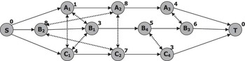
A general JSS problem Jm||C_max is another NP-complete scheduling problem. The JSS problem can be represented in a nice way by a disjunctive graph (Figure 5). The nodes of the graph correspond to operations—let us use node A_i to describe the operation of job A running on machine i (for simplicity reasons, we assume that each job visits each machine at most once). Moreover, each node A_i has a weight that is the processing time of the operation. There are two types of arcs in the disjunctive graph. The conjunctive (solid) arcs represent the precedence relations between operations of the same job. If there is a directed arc (A_i, A_k), then job A has to be processed on machine i before it is processed on machine k. Two operations belonging to different jobs that have to be processed on the same machine are connected by so-called disjunctive (broken) arcs that go in opposite directions. The disjunctive arcs form cliques in the graph; each clique corresponds to one resource. In addition, there are dummy nodes S and T with weights 0 describing the start and end of the schedule. S is connected by conjunctive arcs to the nodes representing the first operations of each job and there are conjunctive arcs from the nodes representing the last operations of jobs to node T.

Figure 5

A disjunctive graph representing a job-shop scheduling problem

The reader should realize that a feasible schedule corresponds to a selection of one arc from each pair of disjunctive arcs such that the resulting graph is acyclic. In particular, the selection of disjunctive arcs in each clique should be acyclic—it corresponds to the sequence in which the operations of particular jobs will be processed on a given resource. Moreover, the longest weighted path from S to T, in which the length is measured as a sum of weights of visited nodes, determines the makespan C_max. This path is sometimes called a critical path. Naturally, the problem of minimizing the makespan reduces to finding a selection of disjunctive arcs that makes the graph acyclic and minimizes the length of the longest path.

We will now present one of the best heuristic algorithms to solve a general JSS problem—a shifting bottleneck heuristic (Adams et al., Reference Adams, Balas and Zawack1988). This algorithm first selects the resource that contributes most to the makespan—a so-called bottleneck resource. Then it finds the best schedule for this resource, that is, a selection of disjunctive arcs from the corresponding clique, adds this selection to the partial schedule, and continues with another resource until all resources are scheduled. Moreover, after scheduling each resource, the already scheduled resources are re-sequenced using the same principle—the removed disjunctive arcs are added back and a new selection for a given resource is found.

The problem of finding the bottleneck resource and generating its schedule can be formulated as the problem 1|r_j|L_max that we already considered. Assume that P_max(k, n) is the longest path from k to n in the current disjunctive graph that includes conjunctive arcs and disjunctive arcs selected in previous iterations of the algorithm. For each not-yet scheduled resource i, the problem 1|r_j|L_max consists of operations allocated to this resource. The processing time of these operations is defined in the JSS problem, the release date , and the due date . Notice that operation cannot start before because this is the earliest time when all preceding operations are finished. In addition, if operation finishes after , this produces a higher makespan. Hence, the bottleneck resource is the resource that contributes to the highest increase of makespan, that is, the resource for which the problem 1|r_j|L_max solves to the largest lateness. The solution of 1|r_j|L_max defines which disjunctive arcs are selected for the resource.

This section describes the basics of traditional scheduling technology. We introduce the scheduling terminology and give some examples of scheduling algorithms. As we have mentioned, there is a large number of different scheduling problems with different techniques to solve them. The reader is referred to the book (Brucker, Reference Brucker2001), which is a detailed catalog of traditional scheduling problems with complexity analysis and references to best algorithms to solve particular problems. The book (Pinedo, Reference Pinedo2002) also describes many scheduling techniques and is appropriate for teaching purposes. Probably the most comprehensive coverage of the advanced topics in scheduling is by Leung (Reference Leung2004).

4.1 Role of constraint satisfaction in planning

One of the difficulties of planning is that the length of the plan, that is, the set of used actions, is unknown in advance, and therefore some dynamic technique that can produce plans of ‘unrestricted’ length is required. Frequently, the shortest plan is being looked for, which is a form of optimal planning. As has been shown in (Kautz & Selman, Reference Kautz and Selman1992), the problem of shortest-plan planning can be translated into a series of logical satisfiability (SAT) problems, in which each SAT instance encodes the problem of finding a plan of a given length. First, we start with finding a plan of length 1, and, if it does not exist, then we continue with a plan of length 2, etc., until the plan is found. There exist criteria to stop these extensions if the plan does not exist (Ghallab et al., Reference Ghallab, Nau and Traverso2004), but for simplicity reasons in this paper we assume that a plan always exists.

Now, the problem of finding a plan of length n can be encoded as a constraint satisfaction problem. The most important steps when designing a constraint model are the selections of variables, their domains, and finally constraints defining consistent tuples of the variables. We will present here the straightforward constraint model that has been described in Ghallab et al. (Reference Ghallab, Nau and Traverso2004) and a more advanced model called CSP-PLAN (Lopez & Bacchus, Reference Lopez and Bacchus2003). For a detailed comparison of these models and their further improvement, the interested reader is referred to Barták and Toropila (Reference Barták and Toropila2008).

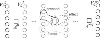
We assume sequential planning in which the world state is described using v multi-valued state variables, the instantiation of which exactly specifies a particular state. A CSP denoting the problem of finding a plan of length n consists of n + 1 sets of the above-mentioned multi-valued variables, with the 1st set denoting the initial state and kth set denoting the state after performing k − 1 actions, for k∈{2,…, n + 1}. We also need n action variables A ^j, in which j ranges from 0 to n − 1, indicating the selected actions (Figure 6).

Figure 6

Base decision variables and constraints modeling plans of length n

The two above-mentioned constraint models (straightforward and CSP-PLAN) differ in the set of constraints used to describe state transitions.

In the straightforward model, we use logical constraints that connect two adjacent sets of state variables through the corresponding action variable between them, that is, for given s, we connect state variable layers V_i ^s and V_i ^s+1, i ∈ {0,…, v − 1}, through the action variable A ^s:

(1)

(2)

where Pre(act)^s and E f f(act)^{s + 1} are conjunctions of equalities setting the values for required state variables corresponding to preconditions of action act in layer s, and its effects in layer s + 1, respectively. We also need constraints representing the frame axioms, that is, constraints that would enforce equalities between those state variables V_i ^s and V_i ^{s + 1}, which are not affected by the selected action A ^s (the frame assumption is implicit in classical planning representations):

(3)

where NonA f f Act(V_i) is the set of actions that does not have state variable V_i among its effects. Please note that this set depends purely on actions’ definition and thus can be pre-computed in advance.

The straightforward model uses separate constraints to describe preconditions and effects of actions and frame axioms specifying that the value of some state variable is not changed by the selected action. There is another more efficient way to describe how the state is changed by merging the constraints for effects and frame axioms into so-called successor state constraints originally described in Reiter (Reference Reiter2001). This method has been used in CSP-PLAN (Lopez & Bacchus, Reference Lopez and Bacchus2003) that was originally proposed as a constraint model for a so-called planning graph (Blum & Furst, Reference Blum and Furst1997). In the planning graph, several parallel actions can be used in each layer provided that these actions do not influence each other. We will present here a simplified version of the constraint model with a single action per layer. The encoding of action preconditions is again using the constraints of type (1). However, in contrast to the straightforward model, we use the successor state axioms instead of effects and frame axioms. In particular, for each possible assignment of state variable V_i ^s = val, val ∈ Dom(V_i ^s), we have a constraint between it and the same state variable assignment V_i ^s−1 = val in the previous layer. The constraint says that state variable V_i ^s takes value val if and only if some action assigned this value to the variable V_i ^s, or equation V_i ^s−1=val held in the previous layer and no action changed the assignment of variable V_i. Formally:

(4)

where C(i, val) denotes the set of actions containing V_i=val among their effects, and N(i) denotes the set NonAffAct(V_i) as described within the previous model.

Notice that the straightforward model uses constraints in the form of implication, which is basically an abbreviation for disjunctive constraints. Disjunctive constraints are known for weak propagation, and therefore the constraint models with disjunctive constraints do not exploit constraint propagation a lot. Hence, search is the prevailing technique for solving such problems. The equivalence constraint in CSP-PLAN leads to a stronger domain filtering and hence this model is more efficient.

Designing a constraint model is just the first step in solving the problem using constraint satisfaction technology. The next step is defining the search strategy, that is, the order in which the variables are instantiated and the order in which the values are tried for the variables. One can use generic search techniques for constraint satisfaction problems, for example, based on fail-first principle; however, it is usually better to exploit the particular structure of the problem. First, one should realize that it is enough to instantiate just the action variables A ^s because when their values are known, the values of the remaining variables, in particular the state variables, are set by means of constraint propagation. Of course, we assume that the values for state variables V_i ⁰ modeling the initial state were set and similarly the state variables V_i ⁿ in the final layer were set according to the goal (the final state is just partially specified and therefore some state variables in the final layer remain un-instantiated). The action variables can be instantiated in increasing order from A ⁰ to A ⁿ⁻¹ to mimic forward planning or in decreasing order from A ⁿ⁻¹ to A ⁰ to mimic regression (backward) planning. For value ordering (selection of action), one can use the planning heuristics designed for other planning algorithms (Ghallab et al., Reference Ghallab, Nau and Traverso2004).

In this section, we have given two examples of constraint models for finding a plan of given length. These models are generated automatically from the description of the planning domain and the planning problem. There also exist handcrafted constraint models, for example, CPlan (van Beek & Chen, Reference van Beek and Chen1999). All these models deal with sequential plans. Constraints are also used in partial order planners (the plan is a partially ordered structure of actions; it is a specific version of plan-space planning) such as the CPT planner (Vidal & Geffner, Reference Vidal and Geffner2004). Last but not least, constraint satisfaction techniques are frequently applied to planning sub-problems such as temporal constraint satisfaction problems (Dechter et al., Reference Dechter, Meiri and Pearl1991) dealing with maintaining temporal relations between actions.

4.2 Role of constraint satisfaction in scheduling

Scheduling is a ‘killer application’ for constraint satisfaction. The success of constraint-based scheduling in real-life applications is thanks to the fact that two research areas, namely OR and AI, combined their complementary strengths in the constraint-based approach. As we saw in the previous sections, the traditional OR approach to scheduling focuses on exploiting the combinatorial nature of a relatively simple mathematical model of the scheduling problem. This leads to a high level of efficiency when solving such problems. The drawback of this approach is that, when mapping the real problem to the mathematical model, usually some degrees of freedom need to be discarded and simplifying assumptions need to be taken. Discarding degrees of freedom may eliminate some interesting solutions while discarding side constraints may lead to unacceptable solutions. In contrast, the AI approach traditionally focuses on general problem-solving techniques so that all degrees of freedom and side constraints are preserved, which may have the disadvantage of poor performance when compared to dedicated solving algorithms.

Constraint satisfaction provides a very good framework for integrating OR techniques in more general AI solving algorithms. The key technology for this integration is based on the notion of global constraints. Global constraints encapsulate a certain part of the CSP and, rather than using a set of constraints to model this sub-problem, a dedicated ‘larger’ global constraint is used that can exploit better the structure of the sub-problem. Global constraints together with sophisticated search techniques are the key power behind the success of constraint-based scheduling. Global constraints provide efficient algorithms to solve well-defined sub-problems while they can be still combined with other constraints modeling the side features of the problem. In this section, we shall give some examples of scheduling global constraints. In particular, we shall describe how the structure of the sub-problem modeled by the global constraint can be exploited in the filtering algorithm.

Let us first describe the base constraint model of a scheduling problem. Recall that a scheduling problem is a decision problem in which we are looking for when and where the jobs will be processed. Jobs typically consist of temporally connected operations that are the basic scheduling objects. For each operation, we can introduce three variables indicating its position in time, namely, the start time, the end time, and the processing time (duration). For operation A, we denote these variables by start(A), end(A), and p(A). We expect the domains for these variables to be discrete (for example, natural numbers representing time), in which the release date and the deadline of the operation make natural bounds for them. It is possible to further restrict the domain by assuming the time windows when the operation can be processed (time windows are a typical example of a real-life side constraint). Though frequently the processing time of operation is a constant number and the start time is enough to fully specify the allocation of operation to time, we prefer to use all three variables to simplify description of the constraints. Speaking about constraints, for operations without pre-emption, the following constraint connects the above three variables: start(A) + p(A) = end(A). The preemptive case is slightly more complicated; the reader may look at (Baptiste et al., Reference Baptiste, Laborie, Le Pape and Nuijten2006, p. 765) for details. If resource allocation is a part of the scheduling problem, then one more variable is required to describe which resource will process the operation: resource(A). Its domain equals the set of numbers, in which the numbers are uniquely assigned to resources. The domain contains just the numbers indicating resources that can process a given operation.

Basically, there are two groups of constraints involved in the model: temporal and resource constraints. Temporal constraints describe the direct temporal relations between the operations, such as the precedence relations. The relation that operation A must be processed before operation B can be modeled using the constraint: end(A)⩽start(B). In the remaining text, we will denote this constraint as A B. It is easy to generalize this constraint to model a more detailed temporal relation with minimal and maximal delays between the operations. Then the constraint has a form min_delay(A, B)⩽start(B) – end(A)⩽max_delay(A, B). When the temporal constraint network is sparse, as is the usual case in scheduling, then standard arc-B-consistency (Lhomme, Reference Lhomme1993) is used to propagate these constraints. For more dense networks, it is more appropriate to use path consistency like algorithms.

Assume we have a unary (disjunctive) resource that can process at most one operation at any time. Two operations A and B processed on the unary resource cannot overlap in time, and therefore either A precedes B or vice versa: A B∨B A. The unary resource can be fully modeled by a set of such disjunctive constraints. Unfortunately, the disjunctive constraints do no propagate well as Figure 7 shows. Three operations are displayed there such that neither pair forbids any sequence (A can be before B as well as after B). As we shall see later, the time window of operation A can be significantly reduced if we consider all operations together.

Figure 7

Example of three operations allocated to a unary resource in which the disjunctive constraints deduce no pruning of time windows

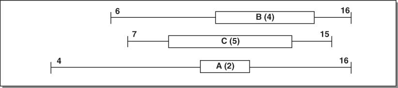
Let us assume hypothetically that operation A is not processed first. Then we must start either with B or C so that the earliest start time is 6. If we now add all processing times of operations A, B, C, which is 11 (=2 + 4 + 5), we get the earliest completion time 17, which is clearly after the latest completion time of all the activities (16). In summary, if we do not start with A, then there will not be enough time to process all activities. The conclusion is that the sequence of operations must start with A, which can be used to prune the time window of A to interval (Bacchus & van Beek, Reference Bacchus and van Beek1998; Baptiste et al., Reference Baptiste, Le Pape and Nuijten2001). This technique, known as edge-finding, can be generalized to a set of operations Ω in the following way:

A Ω means that A must be processed before any operation from Ω; in particular, it must be processed before any Ω′⊆Ω. Therefore, we can restrict the completion time of A in the following way:

A similar rule can be constructed to deduce that A must be processed after Ω:

The above rules are encoded in the global constraint modeling the unary resource. There exist incremental algorithms with the time complexity O(n ³) based on task intervals (Baptiste & Le Pape, Reference Baptiste and Le Pape1996), algorithms with the time complexity O(n ²), for example, the algorithm by (Wolf, Reference Wolf2003) based on the sweep pruning technique, or even edge-finding algorithms with the time complexity O(n.log n) by Carlier and Pinson (Reference Carlier and Pinson1994) or Vilím et al. (Reference Vilím, Barták and Cepek2005), in which n is the number of operations.

Edge-finding is not the only filtering technique for unary constraints. A complementary technique, called ‘not-first/not-last’, deduces that an operation cannot be processed first or last (Torres & Lopez, Reference Torres and Lopez2000). Baptiste and Le Pape (Reference Baptiste and Le Pape1996) designed a not-first/not-last algorithm with the time complexity O(n ²) and Vilím (Reference Vilím2004) proposed a filtering algorithm with the time complexity O(n.log n). Some of the above-mentioned techniques can be extended to cumulative resources, that is, discrete resources with a capacity greater than one (more operations can be processed in parallel). For example, the paper (Baptiste et al., Reference Baptiste, Laborie, Le Pape and Nuijten2006) shows a cumulative version of the edge-finding technique. Other techniques have been proposed particularly for cumulative resources; for example, the energy precedence propagation (Laborie, Reference Laborie2003) combines information about precedence relations and limited capacity of the resource. As we have already mentioned, the big advantage of constraint models is their flexibility in combining constraints describing various aspects of the problem. Therefore, in addition to ‘standard’ features of the problem modeled typically by global constraints, the user may define any other restriction on decision variables.

From the section on constraint satisfaction, it should be clear that the constraint model is not enough to solve the problem; it needs to be accompanied by the search procedure that instantiates the variables. It is possible to use any search strategy developed for constraint satisfaction problems; however, the dedicated search strategies for a class of problems frequently give better results. For example, instead of instantiating the decision variables in the model, the scheduling search strategies are usually based on different branching schemes. As scheduling is basically about finding a sequence of operations, the branching is typically based on deciding which operation is processed before another operation. In particular, if operations A and B are processed on the same resource, we can decide which one will be processed first by exploring two alternatives A B or B A. The question is which pair of operations should be explored first. Smith and Cheng (Reference Smith and Cheng1993) proposed a heuristic based on slack, which describes the flexibility for allocating the operations. More formally, the slack for two operations A and B is defined as:

According to the fail-first principle (select the choice point where no branch leads to a solution with the highest probability), the pair of variables with the smallest slack should be ordered first. According to the succeed-first principle (select the branch that leads to the solution with the highest probability), the ordering with the larger slack should be tried first. This branching scheme requires O(n ²) choices to be resolved during search because each pair among the n operations should be ordered. In Baptiste et al. (Reference Baptiste, Le Pape and Nuijten1995), a different branching scheme for operation selection is studied. Rather than deciding about the order of two not-yet ordered operations, we can decide about the first operation in the resource—we are resolving the disjunction A Ω∨¬A Ω. Again, we can use (resource) slack to find the bottleneck resource: , in which Ω is the set of operations allocated to the resource. The resource with the smallest slack is explored first and the operation with the earliest start time is allocated to the first position (A Ω). If this decision leads to a failure, then the alternative decision (¬A Ω) is used which says that A is not first in the resource. This branching strategy uses O(n) choice points during search. Note finally that resource slack can also be used when deciding about the value of the resource(A) variable. In this case, A is allocated first to the resource with the largest slack (succeed-first principle).

So far we have focused on modeling the feasibility problem, that is, finding a schedule satisfying the resource and temporal restrictions. The optimization problem is usually solved by a branch-and-bound technique in which the objective function Obj depending on variables Vars is represented as a new constraint X = Obj(Vars) with a new variable X that is being minimized (or maximized). The filtering procedure behind the constraint typically restricts the domain of variable X by computing the lower and bound of the objective function for partial instantiation of variables Vars. Again, the relaxation techniques from traditional scheduling that estimate the bounds of the objective function can be transformed into a filtering algorithm of the abovementioned ‘objective’ constraint.

This section has given some examples and techniques of using constraint satisfaction for solving scheduling problems. A more detailed survey can be found in Barták (Reference Barták2005) and Baptiste et al. (Reference Baptiste, Laborie, Le Pape and Nuijten2006), in which planning techniques are also covered. Probably the most comprehensive coverage of constraint-based scheduling is (Baptiste et al., Reference Baptiste, Le Pape and Nuijten2001) in which the filtering algorithms behind the propagation rules for various types of resources are described.

5.1 Integration on planning and scheduling

As we have already mentioned, planning and scheduling are closely related areas. Typically, to solve completely a real-life problem, both planning and scheduling components are necessary. The original planning techniques suppressed the role of limited time and resources and focused on causal relations. However, as the planning techniques become more mature and hence closer to real-life problems, the role of limited time and resources started to be important. Planning with time and resources is now a hot research topic in which scheduling techniques might be exploited. Similarly, so far the scheduling algorithms focused on time and resource allocation and the question how to obtain a set of activities was left apart. Typically, the set of activities is generated by a straightforward algorithm based on the description of environment, for example, using a description of processes of how to manufacture a given part. If there were some options, for example, alternative processes such as outsourcing, the decision was taken by a human operator. However, as production environments are becoming more flexible and complicated, the number of options how to select the activities is increasing and hence the choice of the ‘right’ activities to be scheduled is becoming important. It means that some ideas from planning might be interesting to scheduling as well, for example, in flexible manufacturing environments. Naturally, if complete artificial agents are assumed, such as robots, both planning and scheduling components need to closely cooperate. Hence, not surprisingly, the research on integrating planning and scheduling is driven mainly by the planning community.

5.2 Knowledge vs. software engineering

Traditionally, software engineering plays an important role in the development of planning and scheduling software for real-life applications. The focus is on the software part of the system. In particular, software engineering methods are used to improve the reliability and maintainability of the software, which is definitely important both for the developers and the users of the software. So far much less attention has been paid to the knowledge engineering (KE) part of planning and scheduling. Knowledge engineering deals with the building, maintenance, and development of knowledge-based systems and therefore its goals are close to those of software engineering. The main topics of KE are how to acquire, represent, maintain, and use knowledge.

Knowledge engineering is closely related to artificial intelligence, and therefore it is not surprising that it is more widely used in planning than in scheduling. So far as scheduling deals with ad hoc algorithms for solving particular problems, the KE part is less important. However, as soon as the scheduling software has to deal with a scheduling problem in general, without knowing explicitly to which category the scheduling problem belongs, the role of KE becomes eminent. This is in particular the case of constraint-based scheduling, which is typically oriented to general scheduling problems. For such systems, it is important how to convert data describing parameters of the scheduling problem into an ‘executable’ model that can be solved (Barták et al., Reference Barták, Little, Manzano and Sheahan2007). In addition, the automated extraction of knowledge about the problem is important for efficient problem solving. It could be automated construction of implied constraints (Barták, Reference Barták2007), detection and breaking of symmetries (Puget, Reference Puget2005), or selection of the most promising solving algorithm (Carchrae & Beck, Reference Carchrae and Beck2005).

The role of KE has already been recognized in the planning community in which a competition on KE techniques for planning and scheduling (Barták & McCluskey, Reference Barták and McCluskey2007) is a forum for presenting KE techniques. Knowledge engineering for AI Planning can be defined as the process that deals with the acquisition, validation, and maintenance of planning domain models, and the selection and optimization of appropriate planning machinery to work on them. The typical representatives of KE for planning are the tools for problem modeling, such as the GIPO system (McCluskey et al., Reference McCluskey, Liu and Simpson2003), methods of problem reformulation, such as the methods used in the Fast Downward system (Helmert, Reference Helmert2006), or the methods for learning control knowledge (Borrajo & Veloso, Reference Borrajo and Veloso1996).

5.3 Temporal reasoning

Being able to reason about time is crucial in many real-life problems, such as planning and scheduling. Several approaches have been proposed to reason about temporal information. Temporal constraints have been among the most successful in practice.

In temporal constraint problems, variables either represent instantaneous events, such as ‘when a plane takes off’, or temporal intervals, such as ‘the duration of the flight’. Temporal constraints allow one to put temporal restrictions either on when a given event should occur, for example, ‘the plane must take off before 10 am’, or on how long a given activity should last, for example, ‘the flight should not last more than 2 hours’.

Several quantitative and qualitative constraint-based temporal formalisms have been proposed, stemming from pioneering works by Allen (Reference Allen1983) and by Dechter et al. (Reference Dechter, Meiri and Pearl1991). A qualitative temporal constraint defines which temporal relations, for example, before, after, during, are allowed between two temporal intervals representing two activities. For example, one could say ‘fueling must be completed before boarding the plane’. The quantitative version of this constraint would instead be ‘the time difference between the end of the fueling task and the start of the boarding must be between 5 and 20 minutes’. Disjunctions can be expressed in both formalisms, as in ‘I will call you either before or after the flight’ or ‘I’ll be flying home either between 2 pm and 4 pm or between 6 pm and 8 pm’.

Once the constraints have been stated, the goal is to find an occurrence time, or duration, for all the events in respect of all the constraints. In general, solving temporal constraint problems is difficult. However, there are tractable classes, such as quantitative temporal constraint problems, in which there is only one temporal interval for each constraint (Dechter et al., Reference Dechter, Meiri and Pearl1991). These are problems that consist of a set of variables, and, for each pair of variables, say x and y, at most one constraint of the form a ⩽ x − y ⩽ b, in which a and b are time instants.

5.4 Representing preferences and coping with uncertainty

Preferences and constraints occur in real-life problems in many forms. As said above, constraints are restrictions on the possible scenarios. For a scenario to be feasible, all its constraints must be satisfied. For example, if we want to buy a PC, we may pose a lower limit on the size of its screen. Only PCs that respect this limit will be considered.

Preferences, on the other hand, express desires, satisfaction levels, rejection degrees, or costs. For example, we may prefer a tablet PC to a regular laptop; we may desire having a webcam, and we may want to spend as little as possible. In this case, all PCs will be considered, but some will be more preferred than others. Such concepts can be expressed in either a qualitative or quantitative way.

Preferences and constraints are closely related notions, since preferences can be seen as a form of ‘tolerant’ constraints. For this reason, there are several constraint-based frameworks to model preferences. One of the most general frameworks, based on soft constraints (Rossi et al., Reference Rossi, Van Beek and Walsh2006), extends the classical constraint formalism to model preferences in a quantitative way, by expressing several degrees of satisfaction (that can be either totally or partially ordered). When there are both levels of satisfaction and levels of rejection, preferences may be called bipolar, and can be modeled by extending the soft constraint formalism (Bistarelli et al., Reference Bistarelli, Pini, Rossi and Venable2006).

Preferences can also be modeled in a qualitative way (also called ordinal), that is, by pairwise comparisons. In this case, soft constraints (or their extensions) are not suitable. Other AI preference formalisms are, however, able to express preferences qualitatively, such as CP-nets (Boutilier et al., Reference Boutilier, Brafman, Domshlak, Hoos and Poole2004). Fortunately, CP-nets and soft constraints can be combined, providing a single environment in which both qualitative and quantitative preferences can be modeled and handled.

Specific types of preferences come with their own reasoning engines. For example, temporal preferences are quantitative preferences that pertain to distances and durations of events in time. Soft constraints can be embedded naturally in a temporal constraint framework to handle such a kind of preference (Khatib et al., Reference Khatib, Morris, Morris and Rossi2001; Peintner & Pollack, Reference Peintner and Pollack2004).

While soft constraints generalize the classical constraint formalism providing a way to model several kinds of preferences, this added expressive power comes at a cost, both in the modeling task as well as in the solving process. To mitigate these drawbacks, various AI techniques have been adopted. For example, abstraction theory (Cousot & Cousot, Reference Cousot and Cousot1977) has been exploited to simplify the process of finding the most preferred solution to a soft constraint problem (Bistarelli et al., Reference Bistarelli, Codognet and Rossi2002). In addition, explanations have been considered to ease the understanding of the result of the solving process (Freuder et al., Reference Freuder, Likitvivatanavong, Manuela, Rossi and Wallace2003).

On the modeling side, it may be tedious, or unreasonably demanding, for a user to specify all the soft constraints. In this respect, machine learning techniques have been used to learn the missing preferences from the known ones (Rossi & Sperduti, Reference Rossi and Sperduti1998; Vu & O’Sullivan, Reference Vu and O’Sullivan2007). Alternatively, preference elicitation techniques (Chen & Pu, Reference Chen and Pu2004), interleaved with search and propagation, have been exploited to minimize the user’s effort in problem specification while still being able to find the most preferred solution (Gelain et al., Reference Gelain, Pini, Rossi and Venable2007).

Preferences can be seen as a way to model uncertainty in a constraint problem: if we do not have enough data to know whether a partial assignment of values to variables should be allowed or forbidden, we resort to preferences to, say, something less crisp. However, there are other kinds of uncertainty that can arise and be modeled within a CSP. For example, there could be variables whose value cannot be decided by us. Such variables, usually called uncontrollables, represent events that are not under our control, but can be decided only by Nature or by some other agent.

In temporal constraint problems with preferences, much work has been done to understand how to best deal with uncontrollable events (Vidal & Fargier, Reference Vidal and Fargier1999). In fact, three notions of controllability, that is, strong, weak, and dynamic, are usually considered in this setting. They correspond to more or less pessimistic approaches to deal with this kind of uncertainty.

5.5 Distributed agents

Distributed constraint satisfaction plays an important role in many real planning and scheduling problems where variables and/or constraints must be distributed among a set of agents. Indeed, many real planning and scheduling problems can be modeled as a distributed CSP and solved using distributed CSP techniques. The development of distributed CSP techniques was pioneered by Yokoo et al. (Reference Yokoo, Durfee, Ishida and Kuwabara1992) in their asynchronous BT algorithm.

If all knowledge about the problem can be gathered into one agent, this agent could solve the problem alone using traditional centralized constraint satisfaction algorithms. However, such a centralized solution is often inadequate or even impossible due to inner properties. Faltings and Yokoo (Reference Faltings and Yokoo2005) present some reasons why distributed methods may be desirable:

• • Cost of creating a central authority: A CSP may be naturally distributed among a set of peer agents. In such cases, a central authority for solving the problem would require adding an additional element that was not present in the architecture. Examples of such systems are sensor networks, or meeting scheduling.

• • Knowledge transfer costs: In many cases, constraints arise from complex decision processes that are internal to an agent and cannot be articulated to a central authority. Examples of this range from simple meeting scheduling, where each participant has complex preferences that are hard to articulate, to coordination decisions in virtual enterprisers that results from complex internal planning. A centralized solver would require such constraints to be completely articulated for all possible situations. This would entail prohibitive costs.

• • Privacy/Security concerns: Agents’ constraints may be strategic information that should not be revealed to competitors, or even to a central authority. This situation often arises in e-commerce and virtual enterprisers. Privacy is easier to maintain in distributed solvers.

• • Robustness against failure: The failure of the centralized server can be fatal. In a distributed method, a failure of one agent can be less critical and other agents might be able to find a solution without the failed agent. Such concerns arise, for example, in sensor networks, as well as in web-based applications in which participants may leave while a constraint solving process is ongoing.

Nevertheless, the more cited papers related to distributed CSP make the following assumptions for simplicity in describing the algorithms:

1. 1. Each agent has exactly one variable.

2. 2. All constraints are binary.

3. 3. Each agent knows all constraint predicates relevant to its variable.

Although the great majority of real problems are naturally modeled as non-binary CSPs, the second assumption is comprehensible due to the existence of some techniques that translate any non-binary CSP into an equivalent binary one (Bacchus & van Beek, Reference Bacchus and van Beek1998).

However, the first assumption is too restrictive and the main basic research is focused on small instances, and therefore the following question is straightforward: Is it reasonable to assume to have one variable per agent? (Salido, Reference Salido2007).

Only some works include a set of variables into an agent (Salido & Barber, Reference Salido and Barber2006; Ezzahir et al., Reference Ezzahir, Bessiere, Belaissaoui and Bouyakhf2007). Therefore, more research must be done to solve more realistic problems.

Multi-agent planning and scheduling seems to fall in the intersection of the fields of planning and scheduling, distributed systems, parallel computing/algorithms, and multi-agent systems. However, much of the research appears to build on ideas from either planning or multi-agent systems (and usually not both). From the viewpoint of planning, planning for multiple agents means supporting concurrent actions, and planning by multiple agents means parallelizing a planning algorithm. One might argue that the former has been done and the latter should be solved using parallel computing techniques and is dependent on hardware. On the other hand, from a multi-agent systems perspective, multi-agent planning is not about just solving planning problems but also how agents should behave and interact given that they have plans or planning capabilities.

This survey gives some definitions of constraint satisfaction problems, models, and techniques. It also defines the concepts of planning and scheduling from the AI point of view, as well as the inclusion of constraint satisfaction in planning and scheduling. Finally, some open research issues related to planning, scheduling, and constraint satisfaction are presented.