

INTRODUCTION
Data from paleoclimate proxies constrain the dynamics of Earth’s climate system on time scales inaccessible with the instrumental record. Proxy observations from key intervals of Earth’s past climate, such as the last glacial maximum (LGM) and subsequent deglaciation, allow us to understand how the climate system responds to a change in forcing (e.g., Schmittner et al., Reference Schmittner, Urban, Shakun, Mahowald, Clark, Bartlein, Mix and Rosell-Melé2011; Annan and Hargreaves, Reference Annan and Hargreaves2013; von der Heydt et al., Reference von der Heydt, Dijkstra, van de Wal, Caballero, Crucifix, Foster and Huber2016) and evaluate the ability of climate models to simulate the climate system’s response (e.g., Schmidt et al., Reference Schmidt, Annan, Bartlein, Cook, Guilyardi, Hargreaves and Harrison2014; Annan and Hargreaves, Reference Annan and Hargreaves2015; Harrison et al., Reference Harrison, Bartlein, Izumi, Li, Annan, Hargreaves, Braconnot and Kageyama2015), both of which improve our ability to forecast future climate change (e.g., Masson-Delmotte et al., Reference Masson-Delmotte, Schulz, Abe-Ouchi, Beer, Ganopolski, González Rouco and Jansen2013). Terrestrial proxies are particularly important for assessing how changes in large-scale ocean–atmosphere dynamics manifest at a regional scale in the continental settings that people inhabit and depend upon.
An extensive network of terrestrial climate reconstructions since the LGM exists across the European Alps from pollen, chironomids (midges), organic biomarkers, and inorganic isotope systems (e.g., Bartlein et al., Reference Bartlein, Harrison, Brewer, Connor, Davis, Gajewski and Guiot2011; Blaga et al., Reference Blaga, Reichart, Lotter, Anselmetti and Sinninghe Damsté2013; Heiri et al., Reference Heiri, Brooks, Renssen, Bedford, Hazekamp, Ilyashuk and Jeffers2014; Luetscher et al., Reference Luetscher, Boch, Sodemann, Spötl, Cheng, Edwards, Frisia, Hof and Müller2015; Mauri et al., Reference Mauri, Davis, Collins and Kaplan2015). Despite such an extensive proxy network, our knowledge of deglacial climate conditions in the southern sector of the French and Italian Alps (hereafter referred to as the Maritime Alps) from proxy records is limited. Over the historical period, the Maritime Alps have been characterized by warmer mean annual temperatures, smaller annual temperature amplitudes, lower mean annual precipitation, and snow cover that is thinner and lasts for a smaller fraction of the year than in other Alpine sectors (Durand et al., Reference Durand, Giraud, Laternser, Etchevers, Mérindol and Lesaffre2009a, Reference Durand, Laternser, Giraud, Etchevers, Lesaffre and Mérindol2009b). The Maritime Alps most likely remained the warmest Alpine sector during the late Quaternary, given that the Maritime Alps are ∼6° south of the northernmost eastern Alps and thus would have experienced greater insolation and generally higher temperatures. Warmer overall conditions are consistent with species distribution and phylogeographic models, which suggests that the Maritime Alps remained warmer than other parts of the Alps and functioned as a refugium for plant species during the last glacial period (Casazza et al., Reference Casazza, Grassi, Zecca and Minuto2016). Pollen-based climate reconstructions from four high-elevation sites in the Maritime Alps suggest trends in temperature and precipitation anomalies since the LGM that are broadly similar to those of other Alpine regions (Ortu et al., Reference Ortu, Peyron, Bordon, de Beaulieu, Siniscalco and Caramiello2008). However, these reconstructions are limited by nontrivial variations among the four sites, likely due a combination of nonlocal pollen transport, limited modern analogs at high elevations, and local effects on vegetation cover (Ortu et al., Reference Ortu, Brewer and Peyron2006, Reference Ortu, Peyron, Bordon, de Beaulieu, Siniscalco and Caramiello2008). There is one reconstruction of mean July temperatures from fossil assemblages of chironomids proximal to the Maritime Alps from Lago Piccolo di Avigliana ∼90 km away, but this record is temporally limited to 14–9.5 ka (Larocque and Finsinger, 2008). There are two additional proxy studies from the Maritime Alps that extend into the latest Pleistocene of which we are aware: one reporting fossil pollen assemblages in 16 high-elevation (>1700 m) lakes (Brisset et al., Reference Brisset, Guiter, Miramont, Revel, Anthony, Delhon, Arnaud, Malet and de Beaulieu2015) and one reporting fossil chironomid assemblages from Lac Long Inférieur in France (Gandouin and Franquet, Reference Gandouin and Franquet2002). Neither of these studies interprets the proxies in terms of quantitative climate parameters.
Due to the Maritime Alps’ (1) southerly latitude, (2) generally lower elevations, and (3) proximity to the Mediterranean Sea, the late Quaternary climatic evolution and glacier dynamics in this region may have differed substantially from those in Alpine regions further north and inland (e.g., Kuhlemann et al., Reference Kuhlemann, Rohling, Krumrei, Kubik, Ivy-Ochs and Kucera2008), despite the apparent synchronicity of glacier advances during the LGM and later stadials recorded by moraines across the Alps (e.g., Ivy-Ochs et al., Reference Ivy-Ochs, Kober, Alfimov, Kubik and Synal2007; Kuhlemann et al., Reference Kuhlemann, Rohling, Krumrei, Kubik, Ivy-Ochs and Kucera2008; Federici et al., Reference Federici, Ribolini and Spagnolo2017; Monegato et al., Reference Monegato, Scardia, Hajdas, Rizzini and Piccin2017). Reconstructing temperatures in the Maritime Alps since the LGM would therefore fill a gap in an otherwise extensive network of proxy-based reconstructions of post-LGM climate across the Alps and address the specific question of how climate evolution in the Maritime Alps during deglaciation may have differed from other Alpine sectors. For example, in combination with the positions and chronology of moraines, a well-resolved local temperature record could be used to inform a simple glacier mass balance model for valleys in the Maritime Alps during the deglacial period. With constraints on local deglacial temperatures, a mass balance model could be used to crudely invert for changes in precipitation during deglaciation (e.g., Kessler et al., Reference Kessler, Anderson and Stock2006). This paired temperature–precipitation reconstruction could then be compared with proxy records farther north and inland in the Alps to assess how climate and glacier dynamics varied across the region during deglaciation (e.g., Becker et al., Reference Becker, Seguinot, Jouvet and Funk2016).
In addition to assessing climatic variability during deglaciation across the European Alps, temperature records from an independent proxy could provide tests of different methodologies for reconstructing climate parameters over this time interval. Reconstructions of climate parameters from existing proxies in the European Alps commonly exhibit significant disagreement with climate model simulations prior to the Holocene. Pollen-based reconstructions suggest much colder temperatures, particularly in the winter, than the models predict (e.g., Jost et al., Reference Jost, Lunt, Kageyama, Abe-Ouchi, Peyron, Valdes and Ramstein2005), while models predict higher summertime temperatures than chironomid-based reconstructions during interstadials (Heiri et al., Reference Heiri, Brooks, Renssen, Bedford, Hazekamp, Ilyashuk and Jeffers2014). It is unclear whether these disagreements are attributable to limitations in the global climate models used to simulate paleo-climate, a breakdown in the assumptions of biologically based reconstructions, or some combination of both. Having independent pre-Holocene temperature records in the European Alps that are mechanistically governed by different processes would therefore help in assessing the cause of the current proxy-model discrepancies.
Cosmogenic noble gas paleothermometry is a new geochemical technique for reconstructing past Earth surface temperatures (Tremblay et al., Reference Tremblay, Shuster and Balco2014a). Cosmogenic nuclides are produced by nuclear interactions between target atoms and high-energy cosmic-ray particles, both in Earth’s atmosphere and in the solid Earth. Because the flux of secondary cosmic-ray particles decreases exponentially with depth in rock, production of cosmogenic nuclides is restricted to the uppermost few meters of the Earth’s crust. The near surface production of rare nuclides such as 10Be and 26Al by cosmic-ray particle interactions in common rock-forming minerals like quartz has been extensively developed and utilized over the last 25 years by the geomorphology community to date the surface exposure of rocks and quantify erosion rates (e.g., Granger et al., Reference Granger, Lifton and Willenbring2013). Rare noble gas nuclides such as 3He and 21Ne are also produced in minerals by cosmic-ray particle interactions. In common minerals like quartz and feldspars, these noble gases sometimes exhibit diffusive loss at Earth surface temperatures (Shuster and Farley, Reference Shuster and Farley2005; Gourbet et al., Reference Gourbet, Shuster, Balco, Cassata, Renne and Rood2012; Tremblay et al., Reference Tremblay, Shuster and Balco2014b, Reference Tremblay, Shuster, Balco and Cassata2017) and thus have not been widely used in cosmogenic nuclide studies. However, cosmogenic noble gas–mineral pairs exhibiting open-system behavior (simultaneous production and diffusion) can be utilized used to reconstruct the temperatures that rocks experience while exposed to cosmic-ray particles at Earth’s surface when paired with observations of a quantitatively retained cosmogenic nuclide. In high latitude and/or high altitude environments, theoretical calculations indicate that measurements of 3He in quartz can record temperature variations from the last glacial period to the present (Tremblay et al., Reference Tremblay, Shuster and Balco2014a).
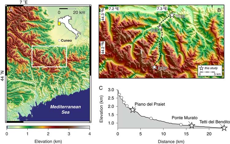
Here, we apply cosmogenic noble gas paleothermometry to investigate temperatures recorded by cosmogenic noble gases since the LGM in the Gesso Valley, located in the southernmost Maritime Alps of Italy approximately 40 km from the Gulf of Genoa in the Mediterranean Sea (Fig. 1). The Gesso Valley was glaciated during the last glacial period. Glacial moraines and other geomorphic features have been mapped throughout the basin (Federici et al., Reference Federici, Pappalardo and Ribolini2003), and cosmogenic 10Be exposure ages have been determined for boulders from three nested moraines that span from the LGM to the Younger Dryas cold period (Federici et al., Reference Federici, Granger, Pappalardo, Ribolini, Spagnolo and Cyr2008, Reference Federici, Granger, Ribolini, Spagnolo, Pappalardo and Cyr2012, Reference Federici, Ribolini and Spagnolo2017). A number of younger, Holocene-age moraines are preserved at higher elevations in the Gesso Valley (Fig. 1), and small glaciers restricted to the highest elevation cirques persist today (Federici et al., Reference Federici, Ribolini and Spagnolo2017). We measured cosmogenic 3He abundances in quartz from a subset of the boulders with 10Be exposure ages from the three previously studied moraines. We also conducted stepwise degassing experiments to quantify the kinetics of 3He diffusion in quartz from these boulders. Because cosmogenic 3He is simultaneously produced and diffusively lost during exposure in the moraines, the “apparent” exposure ages we calculate from the measured 3He abundances are younger than the “true” exposure ages determined from the 10Be measurements. The difference between the apparent and true exposure ages can be used to calculate the integrated effective diffusion temperature (EDT) during exposure. This integrated EDT is the temperature corresponding to the mean diffusivity over a variable temperature history and is therefore a function of the ambient temperature history (Tremblay et al., Reference Tremblay, Shuster and Balco2014a). Paired with sample-specific 3He diffusion kinetics, we use the difference between apparent and true exposure ages to model the permissible integrated EDTs, and by relation temperature histories, of each boulder. The presence of multiple moraines with different exposure ages within the same valley is advantageous, because it allows us to obtain temperature records over different time intervals for an area with a shared climate history.
(color online) (A) Topographic map of the Maritime Alps. Map location is shown in the inset of Italy. White box corresponds to the enlarged view in B. (B) Topography of the Gesso Valley. White stars mark the locations of moraines sampled for this study: Piano del Praiet (PDP), Ponte Murato (PM), and Tetti del Bandito (TDB). Dashed line corresponds to the longitudinal profile shown in C. (C) Longitudinal profile of the Gesso Valley. White stars mark the locations of moraines studied here, as in B; white circles denote additional moraines in the Gesso Valley not studied here. A detailed map of the geomorphic features in the Gesso Valley is available in Federici et al. (Reference Federici, Pappalardo and Ribolini2003).

METHODS
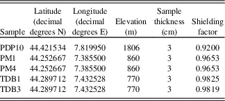
Of the Gesso Valley boulders for which 10Be measurements exist, we obtained archived material (either whole rock or crushed, sieved fractions) from five samples for cosmogenic 3He measurements: one from the Piano del Praiet moraine (PDP10), two from the Ponte Murato moraine (PM1 and PM4), and two from the Tetti del Bandito moraine (TDB1 and TDB3; Fig. 1, Table 1). The 10Be concentration in quartz for PDP10 (223.8 ± 9.6 × 10³ atoms/g, using the 10Be /9Be of Nishiizumi et al. [Reference Nishiizumi, Imamura, Caffee, Southon, Finkel and McAninch2007] for NIST SRM4325) was measured at the Scottish Universities Environmental Research Centre Cosmogenic Isotope Analysis Facility in 2013; all other 10Be concentrations are previously published (Federici et al., Reference Federici, Granger, Pappalardo, Ribolini, Spagnolo and Cyr2008, Reference Federici, Granger, Ribolini, Spagnolo, Pappalardo and Cyr2012). The 10Be exposure ages of these boulders and other boulders from the same moraines have been used to associate the Piano del Praiet, Ponte Murato, and Tetti del Bandito moraines with the Younger Dryas cold period, an intermediate cold period referred to locally as the Bühl stadial at ∼18 ka, and the LGM, respectively (Federici et al., Reference Federici, Granger, Pappalardo, Ribolini, Spagnolo and Cyr2008, Reference Federici, Granger, Ribolini, Spagnolo, Pappalardo and Cyr2012). We separated quartz from other phases using standard crushing, sieving, and magnetic methods, followed by a “frothing” technique commonly used in the ceramics industry to separate quartz from feldspars in the largest sieve fraction that lacked composite grains (Buckenham and Rogers, Reference Buckenham and Rogers1954). Purified quartz was then used to both measure cosmogenic 3He abundances and determine sample-specific 3He diffusion kinetics. All helium isotope measurements were made with an MAP 215-50 sector field mass spectrometer in the Berkeley Geochronology Center Noble Gas Thermochronometry Lab. Gas purification techniques and mass-spectrometer analyses are as described in Tremblay et al. (Reference Tremblay, Shuster and Balco2014b).
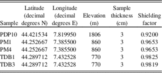
Locations and sample information for moraine boulders in the Gesso Valley previously exposure dated with cosmogenic 10Be, originally reported in Federici et al. (Reference Federici, Granger, Pappalardo, Ribolini, Spagnolo and Cyr2008, Reference Federici, Granger, Ribolini, Spagnolo, Pappalardo and Cyr2012).
For cosmogenic 3He measurements, 100–500 mg aliquots of quartz were weighed and packed into tantalum metal cups with both ends crimped, placed under vacuum in a sample chamber, and heated with a feedback-controlled 150 W diode laser to either 500°C, 800°C, or 1100°C for 15 min until subsequent extractions yielded He signals indistinguishable from the instrumental detection limit. Empty tantalum cup blanks, heated to the same temperatures as the samples, and room temperature procedural blanks were measured throughout each analytical session and subtracted from the sample measurements; 3He blank corrections were typically 2–3 × 10⁴ atoms. Aliquots of air and 3He-spiked helium standards of different manometrically-calibrated pipette volumes were analyzed throughout an instrumental tuning period and used to determine helium sensitivities; sensitivities varied linearly over the pressure range of the sample analyses, estimated by the size of the 4He signal. We propagated uncertainties from the blank corrections and sensitivity regression into the cosmogenic 3He concentrations. We assume that all 3He is cosmogenic, as any magmatic 3He present at the time of mineral formation or nucleogenic 3He (from the reaction 6Li(n,α)3H) produced before reaching the near surface is expected to be lost by diffusion (e.g., Tremblay et al., Reference Tremblay, Shuster and Balco2014b), and any nucleogenic 3He produced at surface temperatures will likely be negligible compared with cosmogenic 3He (Lal, Reference Lal1987).
To determine sample-specific diffusion kinetics, we conducted stepwise degassing experiments on a proton-irradiated quartz grain from each sample. Proton irradiation generates a uniform distribution of 3He in quartz through similar nuclear reactions to those induced by cosmic ray particles but with 10 orders of magnitude or higher production rates, enabling step-degassing diffusion experiments to be conducted on single irradiated quartz grains (Shuster et al., Reference Shuster, Farley, Sisterson and Burnett2004; Shuster and Farley, Reference Shuster and Farley2005; Tremblay et al., Reference Tremblay, Shuster and Balco2014b). We conduct experiments on single grains rather than multigrain aliquots because it allows us to rapidly achieve and then maintain a spatially homogeneous set point temperature, a critical requirement for step degassing experiments. Previous work (Tremblay et al., Reference Tremblay, Shuster and Balco2014b) demonstrates that these single-grain experiments are reproducible for different quartz grains from the same sample. Quartz aliquots were irradiated with a 228.5 MeV proton beam for 6 h at the Francis H. Burr Proton Therapy Center at the Massachusetts General Hospital in December 2015; the total proton fluence for this irradiation was 9.14 × 10¹⁵ p/cm2. The irradiation target design and setup are detailed in Tremblay et al. (Reference Tremblay, Shuster, Balco and Cassata2017). Proton-irradiated quartz aliquots were examined with a binocular microscope, and single crystals lacking visible penetrative fractures and inclusions (fluid or mineral) were selected for stepwise degassing. The dimensions of the chosen grains were measured to estimate the spherical equivalent radius used in later calculations to scale the diffusion length scale. Details of the stepwise-degassing setup and helium measurements are described in Tremblay et al. (Reference Tremblay, Shuster and Balco2014b).
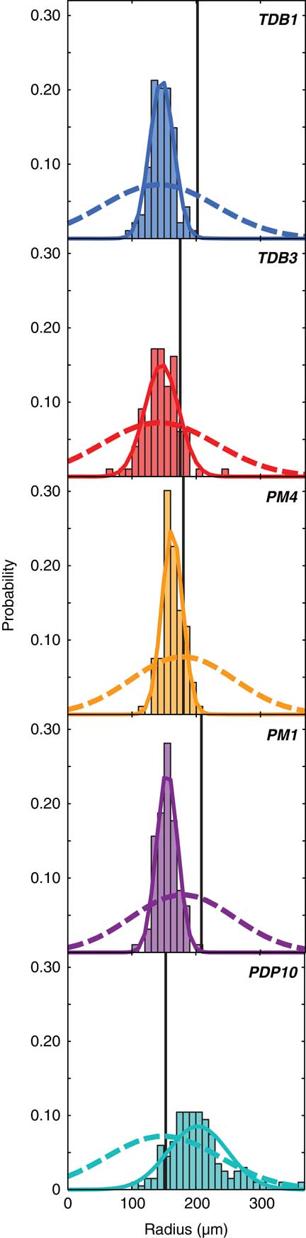
In addition to determining the spherical equivalent radius of the quartz grains used in diffusion experiments, we also determined the spherical equivalent radii of the quartz grains used for cosmogenic measurements and assessed whether these radii are representative of the quartz size distribution in whole rock. Such an assessment is important, because if we significantly reduced the grain size of quartz during the crushing process, this could lead to both an underestimation of the diffusion length scale to which the diffusion experiment size is scaled and missing cosmogenic 3He from our measurements. First, we photographed and measured the dimensions of at least 100 quartz grains from the sieve fraction of each sample used for cosmogenic 3He measurements. We determined major, intermediate, and minor axes of best-fitting ellipsoids using the software ImageJ (Schneider et al., Reference Schneider, Rasband and Eliceiri2012) and calculated the radius of a sphere with the same surface area to volume ratio for each grain. We compared the spherical equivalent radii calculated using this approach with spherical equivalent radii determined from micro X-ray computed tomography (CT) analyses on a smaller number of grains from the same samples, wherein the grains were mapped in three dimensions with a resolution better than 5 μm. CT scans were obtained on the Xradia MicroXCT scanner at the University of Texas at Austin High-Resolution X-ray CT Facility and processed using the software Blob3D (Ketcham, Reference Ketcham2005) as described in Tremblay et al. (Reference Tremblay, Shuster, Balco and Cassata2017). This comparison demonstrates that the ellipsoid approach consistently overestimates the spherical equivalent radius by ∼50%, likely because the ellipsoid method significantly underestimates the surface area of grains. We therefore scaled the spherical equivalent radii from loose-grain measurements by a factor 1.5; the distribution of grain sizes from these measurements are shown in Fig. 2. Also shown in Fig. 2 is the probability distribution of spherical equivalent radii of quartz grains in whole rock. To determine this distribution, we determined circular equivalent radii from measured sectional areas of at least 100 quartz grains in thin sections and inverted the distribution of circular equivalent radii to a distribution of spherical equivalent radii using the code STRIPSTAR and the methodology described by Heilbronner and Barrett (Reference Heilbronner and Barrett2013). For PDP10, the thin section was made from the same sample as the sample crushed for cosmogenic 3He measurements. For the PM and TDB moraines, no whole-rock material from the original samples was preserved; we therefore collected additional material from boulders exposed atop each of these moraines for thin sections and assume that the grain size observed in these samples is representative of the samples for which we have cosmogenic 3He data.
(color online) Grain-size analysis for Gesso Valley samples. Histograms and solid curves denote the distribution of spherical equivalent radii for representative quartz grains (≥100) from the sieve fraction analyzed for cosmogenic 3He abundances. Dashed curves denote the distribution of spherical equivalent radii in whole rock, inverted from the distribution of sectional circles of quartz grains (≥100) measured in thin section. Thin sections were made from the same sample as the crushed fraction, in the case of PDP10, or from a resampled boulder on the same moraine, in all other cases. Vertical black lines denote the spherical equivalent radius of the single quartz grain analyzed in each diffusion experiment shown in Fig. 4.
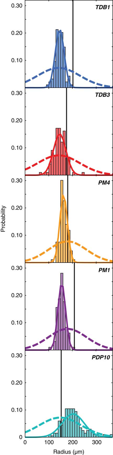
For all samples, the distribution of spherical equivalent radii for the sieve fraction has a smaller standard deviation than the radii determined from thin section measurements (Fig. 2), which is not surprising, given that the sieving process removes larger and smaller grains. With the exception of the PM samples, we find that the mean spherical equivalent radius of quartz in the sieve fraction is equal to or slightly greater than the mean radius determined from thin-section measurements (Fig. 2). The mean quartz radius in the sieve fraction from the PM samples is only slightly smaller than the mean radius from thin section measurements, and the two distributions show significant overlap. Given the good agreement between mean spherical equivalent radii for the sieve fraction and thin section quartz, we assume that the grain size has not been substantially reduced by sample crushing and use the mean and standard deviation of the sieve fraction radii distributions as the appropriate diffusion length scale for modeling the diffusion of cosmogenic 3He in each sample.
RESULTS
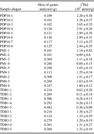
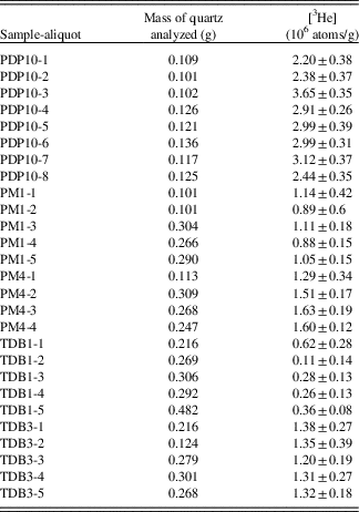
We report measured abundances of cosmogenic 3He in quartz aliquots from each of the Gesso Valley samples in Table 2. We used version 3 (v3) of the online exposure-age calculator code, a more recent version of the code published in Balco et al. (Reference Balco, Stone, Lifton and Dunai2008) that implements the cosmogenic 3He production rate in quartz determined by Vermeesch et al. (Reference Vermeesch, Baur, Heber, Kober, Oberholzer, Schaefer, Schlüchter, Strasky and Wieler2009), to calculate an apparent exposure age from the measured 3He abundance in each aliquot. We assume that the erosion rate is negligible for all boulders sampled, as was assumed in the original publications reporting 10Be exposure ages from these boulders (Federici et al., Reference Federici, Granger, Pappalardo, Ribolini, Spagnolo and Cyr2008, Reference Federici, Granger, Ribolini, Spagnolo, Pappalardo and Cyr2012). Sample coordinates, elevations, thicknesses, and shielding correction factors used in exposure-age calculations are reported in Table 1. In Table 3, we report the weighted mean apparent 3He exposure age for each sample determined using the scaling scheme of Stone (Reference Stone2000). We also recalculated the 10Be exposure ages, normalizing the 10Be concentrations to the isotope ratio standards of Nishiizumi et al. (Reference Nishiizumi, Imamura, Caffee, Southon, Finkel and McAninch2007), using v3 of the online exposure calculator with version 1.1 of the muogenic production rate code and the CRONUS-Earth calibration data set for 10Be production rate (Borchers et al., Reference Borchers, Marrero, Balco, Caffee, Goehring, Lifton, Nishiizumi, Phillips, Schaefer and Stone2016) and the scaling scheme of Stone (Reference Stone2000) (Table 3). Our choice to use the global 10Be production rate calibration data set in Borchers et al. (Reference Borchers, Marrero, Balco, Caffee, Goehring, Lifton, Nishiizumi, Phillips, Schaefer and Stone2016) over a local 10Be production rate calibration (Claude et al., Reference Claude, Ivy-Ochs, Kober, Antognini, Salcher and Kubik2014) does not substantially influence the results presented herein. Because the production rates of 3He and 10Be in quartz are not determined from the same calibration data sets, we use the external uncertainties in exposure ages in all calculations that follow. We divide the weighted mean apparent 3He exposure ages by the 10Be exposure ages (both with external uncertainties) to calculate 3He retention, which represents the fraction of cosmogenic 3He produced during surface exposure that remains in the quartz analyzed (Tremblay et al., Reference Tremblay, Shuster and Balco2014a).
Observations of cosmogenic 3He in Gesso Valley quartz samples.
Apparent 3He exposure ages and retention in Gesso Valley quartz samples. See text for details about the input parameters to the exposure age calculation. Because we have measurements of cosmogenic 3He from multiple aliquots of each sample, we report weighted mean apparent exposure ages with internal uncertainties alongside weighted mean apparent exposure ages with external uncertainties in parentheses. Because we only have one 10Be measurement per sample, we report a single 10Be exposure age for each sample with internal uncertainty alongside external uncertainty in parentheses. Cosmogenic 3He retention is calculated using external uncertainties.

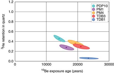
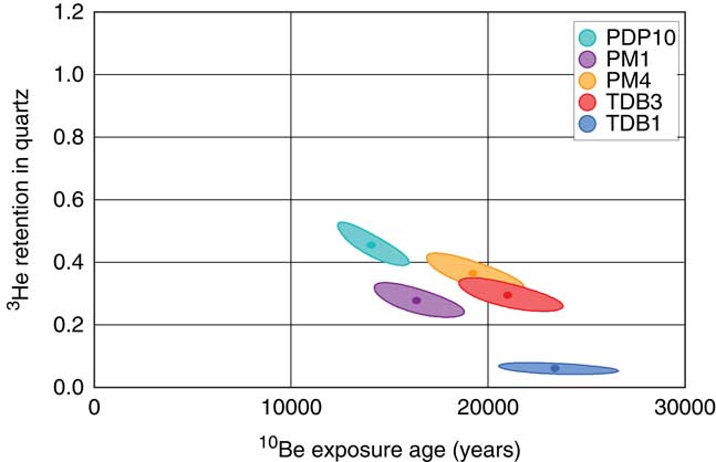
Figure 3 shows 3He retention as a function of exposure duration in the five samples we analyzed. All Gesso Valley samples retain less than 50% of the cosmogenic 3He that was produced during their exposure (Fig. 3, Table 3). Retention generally decreases with increasing exposure duration: quartz from PDP10, sampled from the highest elevation moraine with an exposure age of 14,071 ± 1220 yr, retains 46% of its cosmogenic 3He, while quartz from TDB1, sampled from the lowest elevation moraine with an exposure age of 23,397 ± 2072 yr, retains only 6% of its cosmogenic 3He. In cases in which we have multiple samples from the same moraine, we observe significant intra-moraine differences in 3He retention. PM1 and PM4, both from the Ponte Murato moraine with exposure ages of 16,356 ± 1023 and 19,213 ± 799 yr, respectively, have 3He retentions of 0.28 ± 0.04 versus 0.36 ± 0.04 (Fig. 3, Table 3). Similarly, the two Tetti del Bandito moraine samples TDB1 and TDB3, with exposure ages of 23,397 ± 1085 and 21,003 ± 965, respectively, have 3He retentions of 0.06 ± 0.01 versus 0.29 ± 0.04 (Fig. 3, Table 3).
(color online) Cosmogenic 3He retention as a function of 10Be exposure age in quartz from Gesso Valley moraine samples. Ellipses represent 1σ uncertainty.
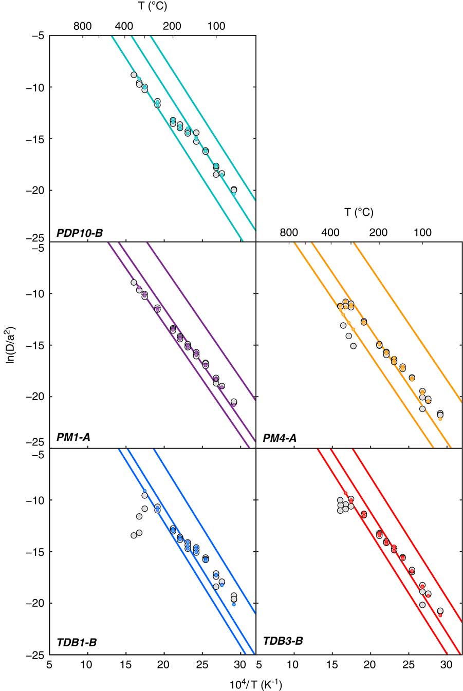
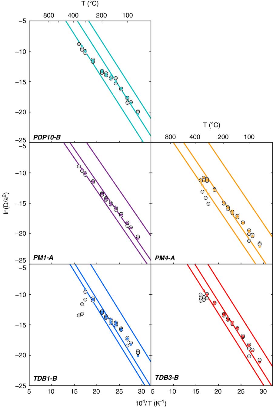
In order to (1) calculate EDTs and infer temperature histories from the observed 3He retention in quartz from each sample and (2) assess the differences in 3He retention between samples from the same moraine, we need to know the diffusion kinetics of 3He in each sample. Figure 4 shows the results of step degassing experiments on proton-irradiated quartz from the Gesso Valley samples in Arrhenius plots in which the natural log of diffusivity, calculated from the cumulative fraction of gas released during each heating step (Fechtig and Kalbitzer, Reference Fechtig and Kalbitzer1966), is plotted as a function of inverse temperature (gray circles).
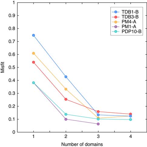
All Gesso Valley quartz samples exhibit some degree of nonlinearity in the Arrhenius plots (Fig. 4). While we do not have a mechanistic explanation or model for this type of complex diffusion behavior (Tremblay et al., Reference Tremblay, Shuster and Balco2014b), multiple diffusion domain (MDD) models (Lovera and Richter, Reference Lovera and Richter1989; Harrison et al., Reference Harrison, Lovera and Matthew1991; Lovera et al., Reference Lovera, Richter and Harrison1991) can reproduce the nonlinearity observed in laboratory degassing experiments and appear to be relevant to 3He diffusive loss over 103–104 year time scales, as demonstrated for a geologic case study for which the temperatures during surface exposure are reasonably well known (Tremblay et al., Reference Tremblay, Shuster and Balco2014b). We constructed MDD models optimized to fit each of the helium step degassing experiments on Gesso Valley quartz samples following the approach outlined in Tremblay et al. (Reference Tremblay, Shuster, Balco and Cassata2017). Figure 5 shows the misfit between the calculated diffusivities from MDD models and the experimentally determined diffusivities as a function of number of diffusion domains, where the misfit statistic was calculated as in Tremblay et al. (Reference Tremblay, Shuster, Balco and Cassata2017). The misfit shown for a given number of diffusion domains is the minimum misfit found after searching over a large range of model parameters (activation energy E a, pre-exponential factor(s) D 0/a 2, and gas fraction(s)).
Arrhenius plots for helium diffusion experiments on Gesso Valley quartz samples. D/a 2 values are normalized to s −1. Experimental data are plotted as gray circles. Diffusivities were calculated using the equations of Fechtig and Kalbitzer (Reference Fechtig and Kalbitzer1966) and the uncertainty propagation outlined in Tremblay et al. (Reference Tremblay, Shuster and Balco2014b). Colored circles and lines denote 3-domain multiple diffusion domain (MDD) models that minimize misfit with the experimental data. Tremblay et al. (Reference Tremblay, Shuster, Balco and Cassata2017) describe the MDD modeling approach used here. (For interpretation of references to color in this figure, refer to the web version of this article).
(color online) Minimized misfit between observed and MDD-modeled 3He diffusivities as a function of number of diffusion domains for Gesso Valley quartz samples. We increased the number of diffusion domains in our MDD models until the addition of another diffusion domain did not significantly reduce the misfit between the observed and calculated diffusivities. For all Gesso Valley quartz samples, we found that increasing the number of domains from 3 to 4 only marginally improved the misfit; therefore, we used 3-domain MDD models in subsequent calculations. For experiment PM1-A, attempts at constructing a 4-domain model yielded two domains with the same pre-exponential factor and thus are the equivalent of the 3-domain model.
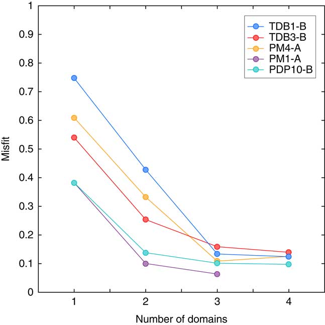
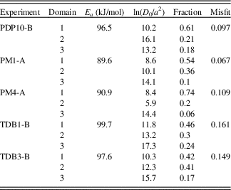
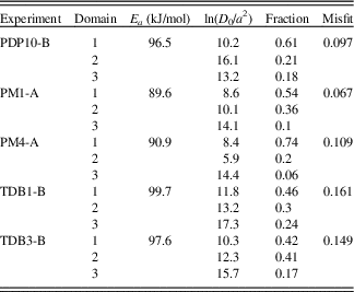
We found that, for all five step degassing experiments, increasing the number of diffusion domains from 1 to 2 and from 2 to 3 significantly reduced the misfit between the observed diffusivities and those calculated with the MDD model (Fig. 5). However, increasing the number of diffusion domains from 3 to 4 did not significantly reduce the misfit between the observed and calculated diffusivities (Fig. 5). For experiment PM1-A, attempts at constructing a 4-domain model yielded 2 domains with the same pre-exponential factor and thus are the equivalent of the 3-domain model. Therefore, for all experiments, we use the diffusion parameters corresponding to the optimized 3-domain model. Lines corresponding to the diffusion parameters of the 3 domains, as well as the calculated diffusivities for the 3-domain models, are shown in color over the experimentally determined diffusivities in Fig. 4. The activation energies, pre-exponential factors, gas fractions, and misfit statistics for these 3-domain models are reported in Table 4.
Three-domain multiple diffusion domain (MDD) model parameters for 3He diffusion experiments in Gesso Valley quartz samples.
As discussed in the “Methods” section, we need to scale the diffusion kinetics determined from the step degassing experiments to the diffusion length scale appropriate for the cosmogenic 3He abundance measurements. In constructing MDD models, we cannot independently parameterize the diffusivity at infinite temperature, D 0, and the diffusion length scale, a. Instead, we model them together as the natural logarithm of the pre-exponential factor in the Arrhenius expression, ln(D 0/a 2), which in an Arrhenius plot corresponds to the y-intercept. Because we cannot independently model the diffusion length scale a, we must make an assumption about how to scale the MDD models appropriately. This is not a problem for the 40Ar/39Ar thermochronometry community in which MDD models were developed, because in almost all cases argon diffusion kinetics and naturally occurring argon isotope abundances are measured in the same mineral grain (e.g., Lovera et al., Reference Lovera, Grove, Mark Harrison and Mahon1997/8). Here, we assume that the diffusion length scale of all domains, and by inference all the pre-exponential factors in a given MDD model, scales with the spherical equivalent radius of the quartz grain analyzed. Theoretically, this implies that diffusion length scale of the most retentive domain (the domain with the lowest ln(D 0/a 2) or intercept in Arrhenius space) is the spherical equivalent radius of the grain analyzed. Practically, this scaling is accomplished as follows:
 $${\left( {{{{D_0}} \over {{a^2}}}} \right)_{{\rm{scaled}}}} = {\left( {{{{D_0}} \over {{a^2}}}} \right)_{MDD}}\left( {{{a_{{\rm{sde}}}^2} \over {a_{{\rm{cosmo}}}^2}}} \right)$$
where a sde is the spherical equivalent radius of the step-degassing experiment quartz grain and a cosmo is the spherical equivalent radius of the quartz grains used for the cosmogenic 3He measurements (Fig. 2).
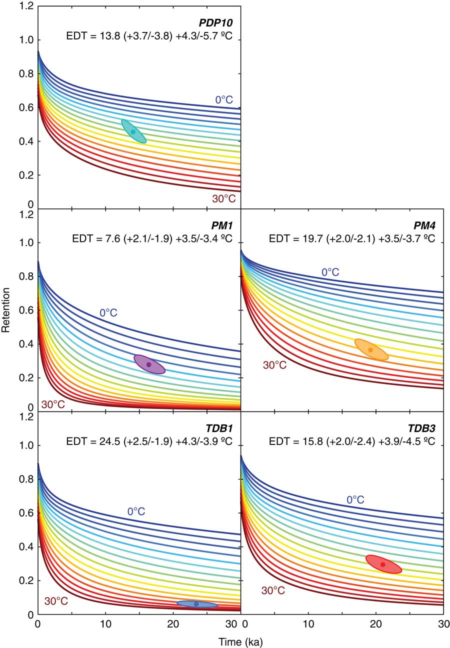
With the scaled, sample-specific diffusion kinetics, we explore possible temperature scenarios to explain the observed cosmogenic 3He abundances in the Gesso Valley samples. To do this, we use forward models of simultaneous production and diffusion to model how cosmogenic 3He retention evolves as a function of exposure duration under different temperature scenarios. We begin with the simplest possible scenario of constant temperature over time. Although constant temperatures are not climatologically realistic, this calculation allows us to determine the EDT, which is the temperature corresponding to the mean diffusivity for a given temperature history that is consistent with the observed cosmogenic 3He retention of each sample. These EDTs are equal to or greater than the true mean temperatures the samples experienced over their exposure durations because of the nonlinear relationship between diffusivity and temperature (Tremblay et al., Reference Tremblay, Shuster and Balco2014a). Figure 6 shows the evolution of 3He retention as a function of exposure duration for constant temperature scenarios in 2°C increments from 0°C to 30°C. These retention evolution curves differ for each Gesso Valley quartz sample for several reasons: (1) each sample has a different set of diffusion kinetics, assuming a 3-domain diffusion model (Fig. 4, Table 4), (2) these sample-specific diffusion kinetics are scaled to different spherical equivalent radii based on the measured grain-size distributions of quartz in the sieve fraction used for cosmogenic 3He measurements (Fig. 2), and (3) the cosmogenic 3He production rate in quartz differs between samples. In each panel of Fig. 6 we report the integrated EDT that agrees with the observed cosmogenic 3He retention in each quartz sample. We provide two uncertainty estimates on this integrated EDT. One set of EDT uncertainties in parentheses accounts for the uncertainty in 3He retention and exposure duration as determined from 10Be measurements; the second set of uncertainties also accounts for uncertainty in the spherical equivalent radius to which the experimentally determined diffusion kinetics are scaled.
(color online) EDTs integrated over the exposure duration of Gesso Valley moraine samples. For each sample, we plot cosmogenic 3He retention as a function of exposure duration for constant EDTs ranging from 0°C to 30°C in 2°C increments, assuming the MDD model diffusion kinetics reported in Table 4. Observed cosmogenic 3He retention ellipses are plotted as in Fig. 3 for comparison. One set of EDT uncertainties in parentheses accounts for the uncertainty in 3He retention and exposure duration as determined from 10Be measurements; the second set of uncertainties accounts for uncertainty in the spherical equivalent radius to which the experimentally determined diffusion kinetics are scaled in addition to the uncertainties in 3He retention and exposure duration.
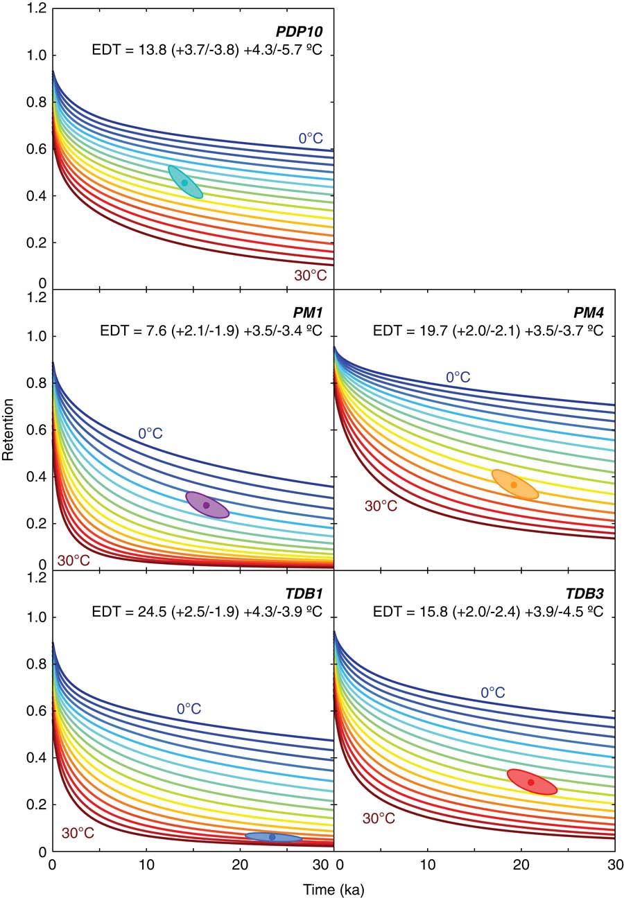
The most readily observable feature of the models in Fig. 6 is that the integrated EDT calculated for each quartz sample is different. This is in part expected, because the different moraines represented by these samples are located at different elevations in the Gesso Valley and thus will experience different temperatures at any point in time due to the atmospheric lapse rate. This may also in part be due to the samples having different exposure durations; for example, a change in temperature between the deposition of the TDB moraine and the PM moraine would only be reflected in the cosmogenic 3He retention and integrated EDT of the TDB moraine samples. Differences in integrated EDT between samples from the same moraine, on the other hand, are unexpected. For PM1 we calculate an integrated EDT of 7.6°C, while for PM4 we calculate a much higher integrated EDT of 19.7°C. Similarly, for TDB1 we calculate an integrated EDT of 24.5°C, while for TDB3 we calculate a much lower integrated EDT of 15.8°C. These intra-moraine discrepancies preclude a straightforward inversion for changes in EDT through time in the Gesso Valley from the inter-moraine differences in 3He retention. We explore possible causes for these intra-moraine discrepancies in the “Discussion” section; here, we compare our observations to modern and paleoclimate observations and simulations to assess whether the EDTs we calculate are plausible for the Gesso Valley since the LGM.
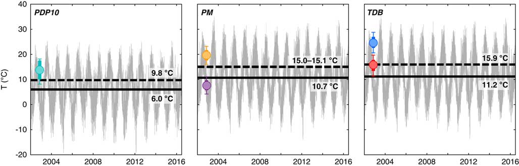
To contextualize these EDTs integrated over the exposure duration of each sample, in Fig. 7 we use modern daily temperature records from 2002 to 2016 to calculate present-day mean temperatures (solid lines) and EDTs (dashed lines) at the elevation of each moraine. We might expect present-day EDTs at each moraine to be comparable to or greater than the EDT integrated over the samples’ exposure durations, considering that mean temperatures during the early, pre-Holocene exposure history of each sample were likely lower than today. However, this expectation may be overly simplistic, as changes in the amplitude of daily and seasonal temperatures since the LGM will also affect the integrated EDTs. Nonetheless, calculation of modern EDTs provides an estimate for the magnitude of the difference between mean temperatures and EDTs due to temperature variations on daily and seasonal time scales in the Gesso Valley.
EDTs calculated from modern meteorological data. In gray we show the time series of mean, minimum, and maximum daily temperatures from 2002 to mid-2016 at the elevations of the PDP, PM, and TDB moraines, scaled from the nearest two meteorological stations using average monthly lapse rates. Solid black bars denote the mean temperature for each time series; dashed black bars denote the modern EDT for each time series calculated using the activation energies of the best-fit MDD models in Fig. 4 and Table 4. EDTs integrated over the exposure duration of each sample are also shown for comparison as circles, with colors for specific samples and 1σ uncertainties as reported in Fig. 6. (For interpretation of the references to color in this figure legend, the reader is referred to the web version of this article.)
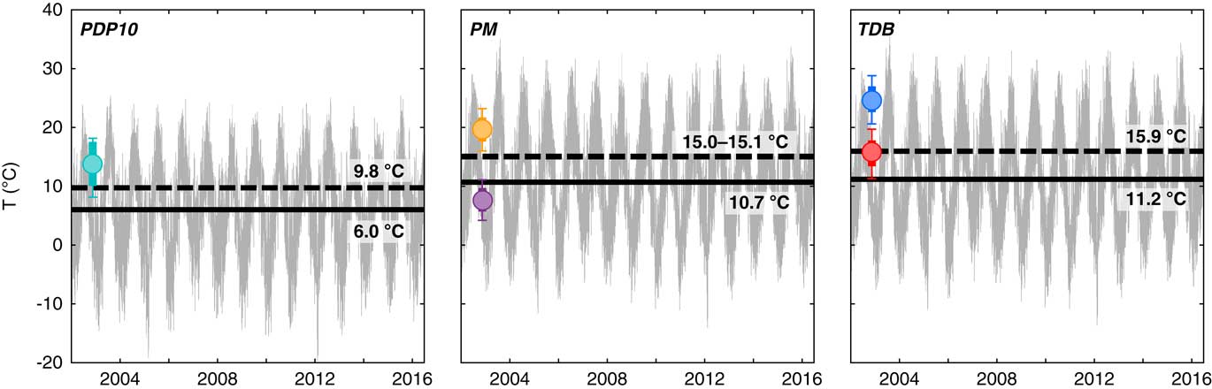
We obtained temperature records at the elevation of each moraine by scaling daily mean, minimum, and maximum temperature data from two meteorological stations within the Gesso Valley: Diga della Piastra (44.227°E, 7.389°N, 959 m) and Diga del Chiotas (44.168°E, 7.334°N, 1980 m). These data are publicly available through the Environmental Protection Agency for the Piemonte Region (arpa.piemonte.gov.it). We scaled the temperature data at Diga della Piastra to the elevation of the TDB and PM moraines and the temperature data at Diga del Chiotas to the elevation of the PDP moraine using monthly average lapse rates determined from the same data set (minimum = 2.8°C/km in December/January; maximum = 6.7°C/km in May) and calculated the modern EDT using these scaled temperature data and the activation energies of the best-fit MDD models in Fig. 4 and Table 4. The modern EDTs at the three moraine elevations are ∼4°C–5°C greater than the mean temperatures, reflecting the effect of daily and seasonal temperature amplitudes on the mean diffusivity and EDT. We do not observe a consistent relationship between modern EDT, calculated at the elevation of each moraine, and integrated EDTs calculated for each sample. For PM4 and TDB1, the modern EDT estimate (15.1°C and 15.9°C, respectively) is several degrees lower than the EDT integrated over each sample’s exposure duration (19.7 + 3.5/–3.7°C and 24.5 + 4.3/–3.9°C, respectively). In contrast, the modern EDT estimates for PDP10 and TDB3 (9.8°C and 15.9°C, respectively) are comparable to the EDTs integrated over their exposure durations (13.8 + 4.3/–5.7°C and 15.8 + 3.9/–4.5°C, respectively), and for PM1 the modern EDT estimate (15.0°C) is several degrees higher (vs. 7.6 + 3.5/–3.4°C).
In addition to comparing the integrated EDTs calculated from observed cosmogenic 3He abundances to modern day EDTs in the Gesso Valley, we can compare our cosmogenic 3He observations to those that would result from (1) temperature histories simulated in general circulation models (GCMs) and (2) temperature reconstructions based on other proxies at nearby locations. GCM simulations and independent proxy reconstructions provide more realistic late Quaternary temperature scenarios with which to test the plausibility of our cosmogenic 3He observations. As cosmogenic noble gas paleothermometry is refined and improved, cosmogenic 3He observations may also be useful for assessing the fidelity of these paleoclimate simulations and reconstructions based on other proxies. For both model and proxy comparisons, the temperature history used to model cosmogenic 3He abundances must be equal in duration to the moraine sample exposure.
Most GCM paleo-experiments simulate climate at a particular point in time, such as the mid-Holocene or LGM; only a handful of GCM simulations have explored transient climate evolution in the Holocene and latest Pleistocene. Here, we model how cosmogenic 3He retention would evolve as a function of exposure duration using seasonal temperature outputs from the TraCE-21ka transient simulation. TraCE-21ka uses the National Center for Atmospheric Research Community Climate System Model version 3 (CCSM3), a synchronously coupled atmosphere–ocean GCM (Collins et al., Reference Collins, Bitz, Blackmon, Bonan, Bretherton, Carton and Chang2006), to simulate the Earth’s climate from the LGM (22 ka) to the present (Liu et al., Reference Liu, Otto-Bliesner, He, Brady, Tomas, Clark and Carlson2009; He, Reference He2011). We obtained mean and maximum seasonal (DJF, MAM, JJA, and SON) temperatures from the TraCE-21ka simulation for the 44.3°N, 7.4°E grid cell including the Gesso Valley. We chose mean and maximum seasonal temperatures for practical reasons (sub-seasonal temporal resolution is computationally unwieldy), but also because these represent endmember EDT scenarios for the moraines in the Gesso Valley. Mean seasonal temperatures represent the low-EDT endmember, as this scenario implies that the mean temperatures represent the full amplitude of seasonal temperature variation and that there is no sub-seasonal (e.g., daily) variability. Maximum seasonal temperatures represent the high-EDT endmember, as this scenario implies that the maximum sub-seasonal temperature simulated during a 3-month interval is the temperature over the duration of that season. We thus expect the observed cosmogenic 3He retention in our samples to be bracketed by the predicted cosmogenic 3He retention from these endmember scenarios, with the mean seasonal temperature scenario placing an upper bound on cosmogenic 3He retention and the maximum seasonal temperature placing a lower bound.
TraCE-21ka simulation temperatures were determined for a mean elevation above sea level for the grid cell, which changed through the simulation as simulated sea level changed. However, the elevation of our sample sites with respect to sea level would have also changed through time, meaning that the relative offset between our sample site elevation and the mean grid cell elevation would have remained constant. We therefore scale the TraCE-21ka simulation temperatures to our sample sites using the present-day difference between the sample site elevations and TraCE-21ka mean elevation assuming the modern seasonal lapse rate determined from the meteorological stations discussed above. The atmospheric lapse rate in the Gesso Valley likely changed between the LGM and the present, especially considering the fact that the valley was more extensively glaciated during part of this interval. Nonetheless, we assume the modern rate, because (1) we have no independent means for assessing how different paleo-lapse rates may have been, and (2) any differences from the modern lapse rate when the valley was glaciated were likely ≤2°C/km (e.g., Davis et al., Reference Davis, Brewer, Stevenson and Guiot2003; Gardner et al., Reference Gardner, Sharp, Koerner, Labine, Boon, Marshall, Burgess and Lewis2009; Loomis et al., Reference Loomis, Russell, Verschuren, Morrill, De Cort, Damsté and Olago2017), which will not be resolvable using our cosmogenic noble gas observations that span ≤1 km in elevation (Tremblay et al., Reference Tremblay, Shuster and Balco2014a).
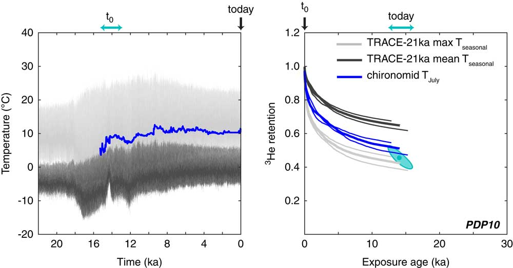
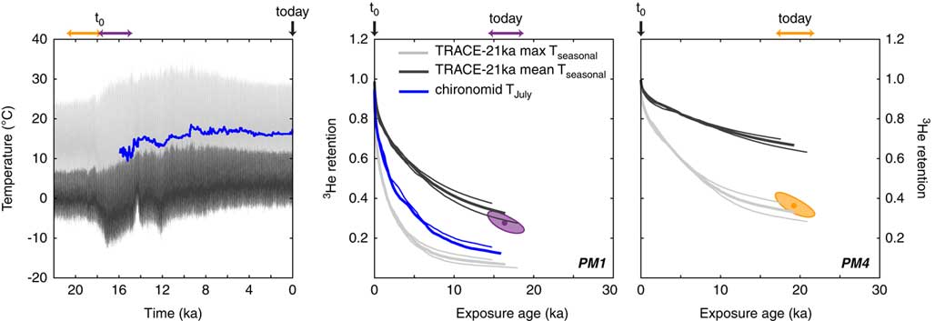
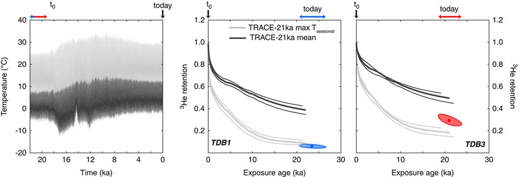
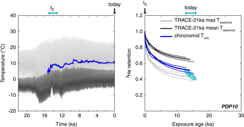
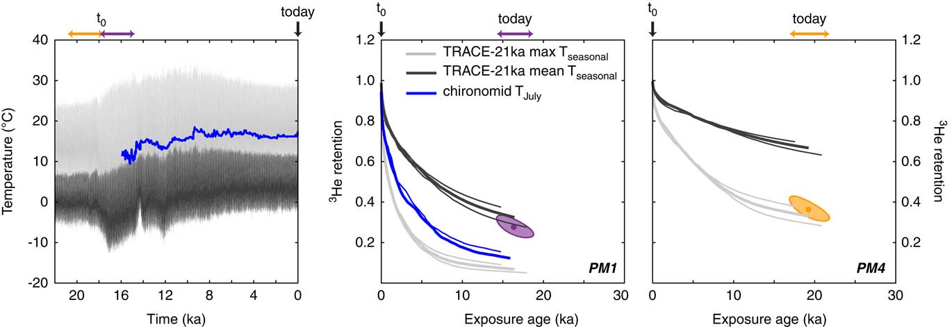
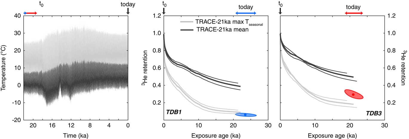
For all Gesso Valley quartz samples, the observed cosmogenic 3He retention is bracketed by the 3He retention calculated assuming mean seasonal temperatures and the 3He retention calculated assuming maximum seasonal temperatures scaled from the TraCE-21ka simulation. For PDP10 (Fig. 8), PM4 (Fig. 9), and TDB1 (Fig. 10), we calculate cosmogenic 3He retention from the TraCE-21ka simulation maximum seasonal temperature that is in agreement within uncertainty with the observed retention in these samples. Cosmogenic 3He retention calculated from the TraCE-21ka mean seasonal temperatures agrees with the observed cosmogenic 3He retention in PM1 within uncertainty (Fig. 9), while for TDB3 the observed cosmogenic 3He retention lies between that predicted from the mean and maximum seasonal TraCE-21ka temperatures.
Cosmogenic 3He retention in PDP10 quartz calculated from scaled TraCE-21ka seasonal temperatures and scaled, spliced chironomid July temperatures. The left panel shows the mean (black) and maximum (gray) seasonal temperature from the TraCE-21ka climate simulation and the mean July temperature (blue) from four spliced chironomid records, scaled to the elevation of PDP10 using modern lapse-rate data and, for the chironomid records, weighted by distance from our study site. The right panel shows the evolution of 3He retention with time assuming the TraCE-21ka and chironomid temperatures represent the EDT experience over PDP10’s exposure duration. Thick retention curves assume the mean exposure duration and grain size for diffusion kinetics scaling; lower thin retention curves assume the +1σ exposure duration and grain size, while upper thin curves assume the −1σ exposure duration and grain size. The ellipse shows the observed retention and exposure duration, as in Fig. 3. (For interpretation of the references to color in this figure legend, the reader is referred to the web version of this article.)
Cosmogenic 3He retention in PM1 and PM4 calculated from scaled TraCE-21ka seasonal temperatures and, in the case of PM1, scaled, spliced chironomid July temperatures. The left panel shows the mean (black) and maximum (gray) seasonal temperature from the TraCE-21ka climate simulation and the mean July temperature (blue) from four spliced chironomid records, scaled to the elevation of PM using modern lapse rate data and, for the chironomid records, weighted by distance from our study site. The right panels show the evolution of 3He retention with time assuming the TraCE-21ka and chironomid temperatures represent the EDT experience over the PM samples’ exposure duration. Thick and thin retention curves are as in Fig. 8. Ellipses show the observed retention and exposure duration, as in Fig. 3. (For interpretation of references to color in this figure, refer to the web version of this article.)
Cosmogenic 3He retention calculated in TDB1 and TDB3 from scaled TraCE-21ka seasonal temperatures. The left panel shows the mean and maximum seasonal temperature from the TraCE-21ka climate simulation, scaled to the elevation of the TDB moraine using modern lapse rate data. The right panels shows the evolution of 3He retention with time assuming the TraCE-21ka temperatures represent the EDT experience over the TDB samples’ exposure duration. Thick and thin retention curves are as in Fig. 8. Ellipses show the observed retention and exposure duration, as in Fig. 3. (For interpretation of references to color in this figure, refer to the web version of this article.)
Lateglacial and Holocene temperatures have been reconstructed from fossil pollen and chironomid records proximal to our study area (e.g., Larocque and Finsinger, 2008; Ortu et al., Reference Ortu, Peyron, Bordon, de Beaulieu, Siniscalco and Caramiello2008). Unfortunately, the pollen-based reconstructions of temperature from high-elevation sites in the Maritime Alps are not numerically reported in full (Ortu et al., Reference Ortu, Peyron, Bordon, de Beaulieu, Siniscalco and Caramiello2008), preventing us from making a direct comparison with our cosmogenic 3He observations. Thus, we use here the chironomid-based July temperature reconstructions from a number of nearby Alpine locations to model cosmogenic 3He retention for comparison with our cosmogenic 3He observations. We spliced together chironomid records from several locations to obtain coeval coverage with samples PDP10 and PM1, which have the youngest 10Be exposure ages of 14,071 ± 1220 and 16,356 ± 1601 yr, respectively. The lack of Alpine chironomid records before 16 cal ka BP prevents us from using chironomid-based July temperature reconstructions to model cosmogenic 3He retention in PM4, TDB1, and TDB3. Like the maximum seasonal temperatures from the TraCE-21ka simulation, we treat the mean July temperature inferred from chironomids as a high-EDT endmember scenario, as this scenario implies that the mean July temperature is representative of subannual temperatures.
The most proximal chironomid-based mean July temperature reconstruction is from Lago Piccolo di Avigliana (LPA), located in the Italian Alps ∼80 km north of the Gesso Valley (45.05°N, 7.38°E, 365 m), where the record extends from 14,200 to 9500 cal yr BP (Larocque and Finsinger, 2008). In order to obtain coeval coverage with the exposure ages of PDP10 and PM1, we spliced the LPA record with chironomid July temperature reconstructions from: Schwarzsee ob Sölden (SOS), a high-alpine lake in the Austrian Alps (46.96583°N, 10.94611°E, 2,796 m) with a chironomid record from 10,200 to –36 cal yr BP (Ilyashuk et al., Reference Ilyashuk, Koinig, Heiri, Ilyashuk and Psenner2011); Lac Lautrey (LAU), a small lake in the French Jura Mountains (46.58722°N, 5.86389°E, 788 m) with a chironomid record from 15,908 to 11,033 cal yr BP (Heiri and Millet, Reference Heiri and Millet2005); and Hinterburgsee (HIN), a subalpine lake in the northern Swiss Alps (46.71833°N, 8.06750°E, 1,515 m) with a chironomid record from 12,210 to 1900 cal yr BP (Heiri et al., Reference Heiri, Tinner and Lotter2004). Like the GCM simulation, we scaled the July temperature reconstructions from each location to the elevations of PDP10 and PM1 using modern lapse rate information, and when temporal overlap occurred between two or more chironomid records, we used an average of the scaled temperatures weighted by the inverse distance between the chironomid sites and our study site.
In Figs. 8 and 9 we show the scaled, spliced July temperature reconstruction using all four chironomid records and the corresponding model for cosmogenic 3He retention in PDP10 and PM1, respectively. We found that different chironomid record splices (e.g., SOS + LPA; SOS + HIN + LPA; SOS + LPA + LAU; SOS + HIN + LPA +LAU) result in very small differences in modeled cosmogenic 3He retention; therefore, only the four-record splice (SOS + HIN + LPA +LAU) is shown. Like the maximum seasonal temperatures from the TraCE-21ka simulation, we model cosmogenic 3He retention from the mean July temperature reconstruction that agrees with our observations from PDP10 and that underestimates the observed 3He retention in PM1.
DISCUSSION
To a first order, the fact that cosmogenic 3He retention calculated with endmember temperature scenarios from a GCM simulation and an independent proxy reconstruction brackets our cosmogenic 3He observations indicates that the 3He observations record ambient temperatures with some accuracy. The observation that our integrated EDTs are not tens of degrees different from modern EDTs in the Gesso Valley calculated with meteorological data also indicates accuracy, as temperature differences between the present-day and the LGM were unlikely to exceed 15°C (e.g., Becker et al., Reference Becker, Seguinot, Jouvet and Funk2016), and post-LGM temperature differences were likely to be much smaller. This first-order agreement suggests that our cosmogenic 3He measurements are providing meaningful information on ambient temperature conditions during exposure. For example, we do not calculate integrated EDTs below 0°C, as we do for cosmogenic 3He measurements made on Holocene-age glacial erratics in Antarctica (Tremblay et al., Reference Tremblay, Shuster and Balco2014a), nor do we calculate integrated EDTs unfeasibly high for Earth surface conditions (e.g., EDTs of 70°C–80°C that we obtain for the Moon [Shuster and Cassata, Reference Shuster and Cassata2015]). However, for the purposes of reconstructing past climate variations, the substantial intra-moraine differences in EDTs are problematic, precluding us from carrying out a straightforward inversion for changes in EDT through time in the Gesso Valley from the inter-moraine differences in 3He retention. For both the PM and TDB moraines, the difference in integrated EDTs between samples from the same moraine is ∼10°C. These intra-moraine differences require explanation.
One possibility is that these intra-moraine temperature differences are real and reflect differential shading of the samples by vegetation, snow cover, or topography. For example, patchy vegetation on a moraine crest may cause one boulder to be fully shaded under a tree canopy, while another boulder tens of meters away remains unshaded. Similarly, boulders nearby to one another might accumulate substantial or insignificant snow cover depending on their relative positioning and shielding from prevailing winds during the wintertime. Unshaded rock samples can experience significantly higher daytime temperatures due to insolation than shaded samples. As discussed in Tremblay et al. (Reference Tremblay, Shuster and Balco2014a), heating of rocks due to incident solar radiation can substantially raise rock temperatures above daily maximum air temperatures. Amplification of temperatures 5°C–10°C above the daily maximum is common in non-desert environments (McGreevy, Reference McGreevy1985; Hall et al., Reference Hall, Lindgren and Jackson2005; Bartlett et al., Reference Bartlett, Chapman and Harris2006; Schwarz et al., Reference Schwarz, Schlink, Franck and Großmann2012). Considering our modern EDT calculations from meteorological station data, if we increase the maximum daily temperature by 5°C or 10°C, we find significant increases in the EDT. For example, using the diffusion kinetics for TDB1, by increasing the maximum daily temperature in the meteorological data by 5°C, we find that EDT increases from 15.9°C to 19.2°C. Increasing the maximum daily temperature by 10°C increases the EDT to 23.0°C, which is within the uncertainty of the EDT integrated over TDB1’s exposure duration. Therefore it is possible that, in the case of the TDB moraine, TDB3 may have been shaded or snow covered during part of its exposure history, while TDB1 was fully exposed to incoming solar radiation throughout its exposure. Similarly, PM1 may have been shaded by vegetation or snow covered during periods of time when PM4 was not.
This interpretation is consistent with the comparison of observed cosmogenic 3He retention to calculated retention from TraCE-21ka and chironomid temperatures. Observations from PDP10, PM4, and TDB1 are closest to the TraCE-21ka simulation maximum seasonal temperature calculations, while observations from PM1 are closer to the calculations with the mean seasonal temperature and observations from TDB3 lie between the predicted 3He retention from mean and maximum seasonal temperature scenarios. We would expect mean temperatures to agree with our cosmogenic 3He observations, as is the case for PM1, if no heating due to insolation occurred. Following the same reasoning, we anticipate that samples experiencing nonzero insolation will have cosmogenic 3He abundances that are lower than what is expected from mean air temperatures, as is the case for PDP10, PM4, TDB1, and TDB3. Likewise, the apparent agreement between the observed cosmogenic 3He retention in PDP10 and the chironomid-based reconstruction of mean July temperatures, which will be significantly greater than mean temperatures throughout most of the year, supports the interpretation that the temperatures experienced by sample PDP10 exceeded air temperatures during PDP10’s exposure to cosmic ray particles. A more precise relationship between insolation-induced daily rock temperature amplifications and maximum seasonal air temperatures or mean July air temperatures could be obtained by monitoring in situ rock temperatures adjacent to meteorological stations, such that these temperature scenarios could be adjusted and provide more information than just a high-EDT endmember.
We note that shading from solar radiation and shielding of cosmic rays are not equivalent. Vegetative cover can have a substantial effect on heating by insolation, but in most cases a negligible effect on cosmogenic nuclide production rates due to its relatively low density. Similarly, thin snow cover will not substantially affect cosmogenic nuclide production rates but will cause rock temperatures to differ substantially from air temperatures. Thick snow cover (≥1 m) will affect both production rates and temperatures. Today, there is significant vegetation cover on the TDB and PM moraines, but no cover at PDP. Unfortunately, we have no way of assessing the degree of vegetation cover on the TDB and PM moraines before the modern era, and no way to assess the past degree of snow cover for all moraines (although observations of in situ 14C in quartz could help address snow cover; e.g., Hippe et al., Reference Hippe, Ivy-Ochs, Kober, Zasadni, Wieler, Wacker, Kubik and Schlüchter2014). Topography can shield rocks from cosmic ray particles, but these effects are accounted for in our calculations of cosmogenic nuclide production rates (Table 1); in contrast, we have not accounted for the effects of topographic shading on rock surface temperatures. We do not have detailed enough locations for the TDB and PM samples to identify the original boulders that were sampled and assess differences in topographic shading, although we suspect this would be secondary to vegetation and snow cover effects.
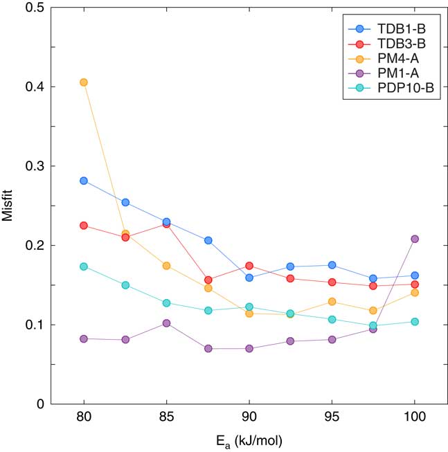
Another possible explanation for the intra-moraine differences is that our MDD model representations of helium-diffusion kinetics in Gesso Valley quartz samples are inaccurate and/or inadequate. The MDD models we construct are inherently non-unique, and while the models we use minimize the misfit between the observed and calculated diffusivities in our step-degassing experiments for a given number of domains, comparable fits can be achieved over a range of diffusion parameters. To illustrate this, in Fig. 11 we show minimized values of MDD model misfit, calculated using the misfit statistic defined in Tremblay et al. (Reference Tremblay, Shuster, Balco and Cassata2017), as a function of activation energy E a for 3 domain models fit to each of the step degassing experiments shown in Fig. 4. For most of the step degassing experiments, there exist a broad range of activation energies (and associated pre-exponential factors and gas-release fractions) over which the misfit with the MDD model changes only slightly; these changes in misfit are much smaller than the change in misfit associated with increasing the number of diffusion domains and the model complexity (Fig. 5).
(color online) Minimized misfit between observed and MDD-modeled 3He diffusivities as a function of activation energy Ea for Gesso Valley quartz samples, assuming a three domain diffusion model. Pre-exponential factors and gas fractions for each domain covary with Ea; we show misfit as a function of Ea because it is assumed to be common to all diffusion domains in our modeling approach.
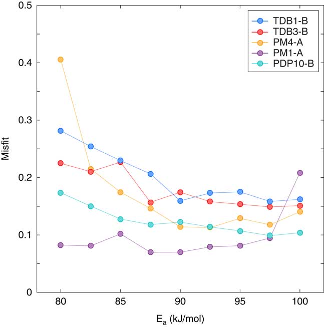
For example, the MDD misfit for the PM1-A step-degassing experiment ranges between 7.0% and 10.2% between activation energies of 80 and 97.5 kJ/mol (Fig. 11). The MDD diffusion kinetics we use in the forward models for PM1 quartz presented earlier assume an activation energy of 89.6 kJ/mol. If instead we use a different set of diffusion kinetics for a 3-domain model that yields a comparable misfit with the step degassing experiment (E a = 97.5 kJ/mol; ln(D 0/a 2) = 12.2, 10.1, 16.8; f gas = 0.45, 0.44, 0.11; Misfit = 0.095), we calculate an integrated EDT from the cosmogenic 3He retention in PM1 quartz of 17.8 (± 2.3) +3.8/−3.9°C, which is in agreement with the integrated EDT we calculated for PM4 (Fig. 6). This highlights how sensitive the temperatures we calculate from an observed amount of cosmogenic 3He retention are to the diffusion kinetics we use. While different MDD models might reproduce diffusivities observed in laboratory step-degassing experiments comparably well, the downward extrapolation of these models results in significantly different diffusivities at the temperatures characterizing Earth’s surface. This suggests that some or all of the intra-moraine differences in integrated EDTs could be attributed to uncertainties in how we extrapolate laboratory-determined diffusion kinetics. Given that we do not yet have a mechanistic understanding of what controls the complex noble gas diffusion behavior we observe in our experiments, discriminating between different MDD models of comparably good fit (and even assessing whether MDD models adequately represent the processes responsible for complex behavior) is difficult at this stage.
A third possible explanation for the intra-moraine variation could arise from our grain size analysis and scaling of MDD models. Uncertainty in the physical significance of our MDD models translates into an uncertainty in our assumptions about how to scale our MDD model fits from step degassing experiments to the cosmogenic 3He measurements. However, because we have scaled the results of each experiment using the same assumptions as in Eq. 1, the effects will be systematic. Similarly, the factor of 1.5 we applied to estimated spherical equivalent radii of quartz from the sieve fractions, based on different approaches to estimate surface area to volume ratios and ground truthing with X-ray CT data, will have systematic effects on all integrated EDTs. Assuming that the MDD model scaling and correction applied to sieve fraction measurements are appropriate, we must also consider the possibility that our grain-size analysis for the PM and TDB samples does not represent the actual grain size and diffusion length scale of quartz in these samples. Since we did not have whole rock material from the original PM and TDB samples, we made thin sections from other boulders collected from the PM and TDB moraines to compare with the size distributions of quartz in the sieved fraction. While there is good agreement between the mean spherical equivalent radii of quartz measured in these thin sections and in the sieve fractions, it is possible that in the original sample, the mean quartz size before crushing was much larger. As a sensitivity test, we again use PM1 as an example. To obtain an integrated EDT for PM1 equivalent to that calculated for PM4 of 19.7°C, we must increase the spherical equivalent radius assumed for the cosmogenic 3He measurement by 110% (without changing the spherical equivalent radius for PM4). While such a dramatic underestimation of the PM1 grain size, and more generally >100% uncertainty in all our PM and TDB grain-size analyses, seems unlikely, we cannot rule out such a possibility, given that whole rock material from these samples was unavailable.
As a final potential source of intra-moraine variation, the moraine boulders that we sampled may have more complex exposure histories than we allow for in our production and diffusion models, either due to cosmogenic 10Be and 3He inheritance or due to nonzero erosion rates that vary between boulders. More complex exposure histories are plausible for all three moraines, as the 10Be exposure ages from a given moraine do not overlap within their internal uncertainties (Table 3). Although we only studied one boulder from the PDP moraine, cosmogenic 10Be measurements for four additional PDP boulders also exhibit dispersion that cannot be explained by measurement uncertainty alone (Federici et al., Reference Federici, Granger, Pappalardo, Ribolini, Spagnolo and Cyr2008). PDP10, the sample studied here, has the oldest exposure age of the five boulders with 10Be measurements. We do not have measurements of additional cosmogenic nuclides (e.g., in situ 14C) to test whether our samples exhibit evidence for complex exposure. Nonetheless, we can explore what effects inheritance and nonzero erosion might have on our cosmogenic 3He observations and the EDTs we calculate from them.
Inheritance would most likely affect the boulders from each moraine with the oldest apparent 10Be exposure ages: PDP10, PM4, and TDB1. The cosmogenic 3He observations from these boulders yield higher integrated EDTs than other boulders from the same moraine (in the case of PM4 and TDB1) and are closest to the 3He retention calculated using the high-EDT endmember scenarios (maximum seasonal temperatures from TraCE-21ka and mean July temperatures from spliced chironomid records). For inheritance to explain these observations and the intra-moraine differences in integrated EDT, the quartz in these boulders would have to lose a substantial proportion of their inherited 3He relative to inherited 10Be. This is not unreasonable considering that temperature-dependent diffusive loss would also affect cosmogenic 3He produced prior to boulders being deposited in a moraine; thus we consider inheritance to be a viable option to explain some of the intra-moraine discrepancies we observe.
In contrast, nonzero erosion rates will likely affect the boulders from each moraine with the youngest apparent 10Be exposure ages: PM1 and TDB3. The cosmogenic 3He observations from these boulders yield lower integrated EDTs than other boulders from the same moraine and are closer to the 3He retention calculated using the low-EDT endmember scenario (mean seasonal temperatures from TraCE-21ka). If we assume that 15 cm of material has been eroded since the initial exposures of PM1 and TDB3—corresponding to the depth at which daily temperature oscillations typically become negligible in rock (Tremblay et al., Reference Tremblay, Shuster and Balco2014a)—and that the exposure ages calculated from 10Be measurements from PM4 and TDB1 are the respective true exposure ages, we can recalculate the 10Be exposure age, 3He apparent exposure age, and 3He retention for PM1 and TDB3. This results in an increase in 10Be exposure age (e.g., from 16,356 ± 1023 to 18,821 ± 1335 for PM1), but not a substantial decrease in 3He retention (e.g., from 0.28 ± 0.04 to 0.25 ± 0.04 for PM1). As a consequence, the integrated EDTs we would calculate for these samples including the effects of erosion would not be substantially higher than those we calculated assuming no erosion. A similar effect is expected if, rather than the boulder surfaces themselves having eroded, the boulders were initially shielded by a variable thickness of sediment cover that has since eroded (e.g., Putkonen and Swanson, Reference Putkonen and Swanson2003; Heyman et al., Reference Heyman, Stroeven, Harbor and Caffee2011). Thus the effects of variable erosion seem unlikely to fully explain the intra-moraine differences we observe.
In summary, there is substantial intra-moraine variability in the integrated EDTs we calculate from our cosmogenic 3He observations that requires explanation. We have outlined four major sources of uncertainty in our approach that could explain these intra-moraine variations. Ultimately, these potential sources of uncertainty are too under-constrained at this time to allow for a straightforward interpretation about the climate history of the Maritime Alps during deglaciation from our cosmogenic noble gas data. Nonetheless, we calculate integrated EDTs for all samples that are bracketed by plausible endmember EDT scenarios for the Gesso Valley based on mean and maximum seasonal temperatures from the TraCE-21ka simulation and on chironomid-derived mean July temperature reconstructions. The trend toward the high-EDT endmember scenarios for all samples except PM1 is not surprising, given that we expect integrated EDTs to exceed the mean ambient temperatures in a sample’s exposure history because of the nonlinear dependence of diffusivity on temperature. The observation that our integrated EDTs are not drastically different from modern EDTs in the Gesso Valley is also encouraging, given the magnitude of plausible temperature differences between the LGM and today. Collectively, these results demonstrate promise for the application of cosmogenic noble gas paleothermometry in paleoclimate studies, provided that the four major sources of uncertainty we have detailed are accounted for in future applications.
CONCLUSIONS
Integrated EDTs since the LGM in the Gesso Valley, calculated from our observations of cosmogenic 3He concentrations in quartz, range from 8°C to 25°C and are consistent with what we expect from modern meteorological station data, a GCM simulation of Earth’s climate since the LGM, and data from independent proxies in the region. Nonetheless, there are nontrivial differences between the integrated EDTs we calculate, particularly for samples from the same moraine, that require explanation. We identify four major potential sources of uncertainty that could account for these discrepancies: (1) the fact that we have not accounted for variations in radiative heating of the boulder surfaces across samples due to differential shading, (2) limitations in our understanding of and ability to model and extrapolate helium diffusion kinetics when complex behavior is observed, (3) uncertainties associated with our quartz grain-size analyses, and (4) unaccounted-for erosion or cosmogenic inheritance. At this stage, all four of these possibilities could be contributing to intra-moraine and inter-moraine variability in reconstructed temperatures. Because of these uncertainties, and the fact that we have no cosmogenic 3He observations from younger moraines that record only Holocene temperatures in the Gesso Valley, it is difficult to fully compare our results with the TraCE-21ka and chironomid temperature records or to invert our results directly for changes in EDT through time in the Gesso Valley from the inter-moraine differences in 3He retention. As a consequence, it is not yet possible to use our data set to test the hypothesis that the post-LGM climate evolution and glacier dynamics of the Maritime Alps differed from other Alpine regions. These results nonetheless demonstrate first-order accuracy in the temperatures recorded by cosmogenic noble gas paleothermometry and highlight major sources of uncertainty that can be addressed in future applications to improve how cosmogenic noble gas paleothermometry contributes to paleo-climate studies.
ACKNOWLEDGMENTS
MMT and DLS acknowledge support from the National Science Foundation (NSF) Petrology and Geochemistry Program (EAR-1322086 to DLS), the UC Berkeley Larsen Grant, and the Ann and Gordon Getty Foundation. MMT was supported by an NSF Graduate Research Fellowship. MS acknowledges support from the Royal Society (IE150603), the Leverhulme Trust (IAF-2016-001), and NERC (CIAF 9092.1010). AR acknowledges support from the University of Pisa fund PRA (2017). M. Uebner and S. Woodmansee are thanked for help with sample preparation. We also thank Associate Editor Kathleen R. Johnson, Jakob Heyman, and an anonymous reviewer for constructive feedback on this work.