1. Introduction
The research funding system has been dramatically reformed over the past two decades. Traditionally, research funding has been classified into two categories: (i) noncompetitive block grants for research institutions and (ii) competitive funding for research projects. However, many new funding methods have recently been introduced, and the distinction between them has become ambiguous. Securing funding for research has also become highly competitive (Larrue et al. Reference Larrue, Guellec and Sgard2018). The effects of such reforms on the efficiency of the scientific community remain to be evaluated.
Project-based research funding by lottery is a recently introduced method in which funds are awarded to a project chosen by lottery rather than by peer review. It was first introduced by the Health Research Council of New Zealand in 2013 and was later adopted by several agencies (Adam Reference Adam2019). The idea of utilizing a lottery system has been repeatedly proposed in different disciplines (for a review, see Avin [Reference Avin2019b]). One of the main reasons for this is the difficulty of peer-review systems in evaluating proposals reliably. For example, Graves et al. (Reference Graves, Barnett and Clarke2011) analyzed the peer-review scores of the National Health and Medical Research Council of Australia and found variability in the final decisions. By randomly sampling the original review scores of the review panels, they obtained 1,000 hypothetical panel judgments for each proposal and found that only 255 proposals were always funded among 620 proposals that were actually funded. Another example by Pier et al. (Reference Pier, Markus Brauer, Anna Kaatz, Nathan, Ford and Carnes2018), which replicated the peer-review process of the National Institutes of Health (NIH), showed less consistency among reviewers’ evaluations. In addition, it has been argued that a lottery system has two advantages over a peer-review system (Fang and Casadevall Reference Fang and Casadevall2016). First, unlike peer review, a lottery system has no inherent systematic biases,Footnote 1 whereas the peer-review process may have several biases. It has been claimed that the peer-review process is biased toward conservative approaches, such that novel ones tend to be suppressed (Brezis Reference Brezis2007; Gillies Reference Gillies2014; Fang and Casadevall Reference Fang and Casadevall2016). Furthermore, there may be additional biases concerning gender or race (Brezis Reference Brezis2007; Fang and Casadevall Reference Fang and Casadevall2016). A lottery system is considered an effective way to reduce these detrimental biases. Secondly, a lottery system may help reduce the burdens that the peer-review process imposes on applicants, reviewers, and administrators. Because applicants are currently required to submit very detailed proposals, the preparation and review costs are high. A lottery system may reduce these costs because heavily detailed proposals are no longer necessary. Although some rough prescreenings before the lottery may be required to exclude inappropriate proposals, the information necessary for such screenings would be much less than that required for a full peer-review process.Footnote 2
The effect of various funding strategies on the productivity of the scientific community is beginning to be discussed in the field of philosophy of science. Since the pioneering work by Kitcher (Reference Kitcher1990), philosophers of science have investigated the division of cognitive labor (i.e., the diversity of approaches that scientists take) using theoretical models (Kitcher Reference Kitcher1990; Strevens Reference Strevens2003; Weisberg and Muldoon Reference Weisberg and Muldoon2009). Recently, Avin (Reference Avin, Mäki, Votsis and Ruphy2015, Reference Avin2019a) focused on the role of funding strategies in realizing an efficient division of cognitive labor and compared the performance of various funding strategies. Using the epistemic landscape model (Weisberg and Muldoon Reference Weisberg and Muldoon2009), he argues that a funding system combining peer review and lottery maximizes the productivity of the scientific community. This result may be expected, considering that there are arguably two activities that are important for the efficiency of the scientific community. One is to investigate well-established research topics (exploitation), and the other is to search for undiscovered topics (exploration). The peer-review process would enhance the former type of research because it would favor the conventional approach. On the other hand, a lottery system would help the latter type of research, which may not be awarded by peer review. Therefore, it is reasonable to assume that combining these methods would support the scientific community by enhancing both types of research in parallel.
However, this cannot be fully concluded because Avin’s model does not consider conventional baseline funding, such as block grants. Because such grants are also distributed without bias and do not impose significant costs, they would have similar advantages to a lottery system. Moreover, unlike a lottery system, baseline funding would promote long-term research because it stably assigns a relatively small amount of funds to all scientists, whereas a lottery system assigns a larger sum to only a limited number of scientists. Given the putative benefits of baseline funding, it is important to elucidate the relative efficiency of these strategies.
The current article aims to compare resource distribution systems based on lottery and baseline funding from the perspective of the efficiency of the scientific community. Following Avin (Reference Avin, Mäki, Votsis and Ruphy2015; Reference Avin2019a), I constructed a simulation model that extends the epistemic landscape model. It is more general than Avin’s model and can represent a variety of funding strategies, thus allowing for comparisons among them. It can also incorporate the effects of new researchers’ entry into a scientific discipline. In Avin’s model, only the entrance of researchers from other disciplines seems to be considered (see section 3 for more details). However, the difficulty in entering a discipline may depend on the character of each discipline, and new researchers may also come from the same discipline (i.e., graduates from one of the laboratories). Thus, I introduce a parameter that explicitly represents these aspects and investigate their effects. The results from the model suggest that conventional baseline funding outperforms lottery funding in many cases. The results also indicate that the optimal balance of competitive and noncompetitive funding largely depends on the “openness’’ of a specific discipline to researchers from other disciplines.
In the subsequent section, I briefly review previous studies on the division of cognitive labor discussed in philosophy of science, especially focusing on the epistemic landscape models. Recent studies by Avin and some of the limitations of his model have also been discussed. Finally, I introduce a more general model that can represent both lottery and baseline funding, compare their efficiency under various conditions through simulation experiments, and provide general conclusions based on the outcomes.
2. Models for the division of cognitive labor
Since Kitcher’s (Reference Kitcher1990) pioneering work on the division of cognitive labor, this topic has been widely discussed in philosophy of science. Among the most popular approaches in this field is the epistemic landscape model, first introduced by Weisberg and Muldoon (Reference Weisberg and Muldoon2009). Whereas Kitcher’s approach concerns the division of labor in pursuing different approaches to solve a certain problem, the epistemic landscape model concerns the division of labor in exploring research projects in a particular discipline. In this section, I review studies on the division of cognitive labor, especially focusing on the epistemic landscape model, and identify some problems. In section 2.1, I discuss epistemic landscape models that focus on the role of the division of research strategy (i.e., how scientists choose their research projects) in realizing the optimal division of labor. Although the division of research strategy can enhance the efficiency of the scientific community (e.g., Pöyhönen Reference Pöyhönen2017), it has been pointed out that the division of research strategy is difficult to control in the real scientific community (Heesen Reference Heesen2019). A more promising approach would be to investigate the role of extrinsic factors, such as funding agencies, in realizing the optimal division of labor. In section 2.2, I discuss such an approach by Avin, who first introduced a funding agency into the epistemic landscape model and argued that the partial introduction of a lottery system in the funding distribution is beneficial in many situations (Avin Reference Avin, Mäki, Votsis and Ruphy2015, Reference Avin2019a). However, I point out that some important aspects of the scientific community are missing in his model, which would affect his conclusions.
2.1. Epistemic landscape models
Weisberg and Muldoon (Reference Weisberg and Muldoon2009) considered the division of the scientists’ workload among various research projects on the same broad topic.Footnote 3 To model this situation, the authors introduced an epistemic landscape model (see figure 1 for an example of a three-dimensional landscape). The epistemic landscape model of n dimensions is composed of an
 $n - 1$
-dimensional grid where each grid point represents a single research project characterized by the combination of
 $n - 1$
features (research question, instruments, methods of analysis, background theories, and so on) and a one-dimensional axis that represents the significance of each project that scientists would discover once it is completed. The landscape of significance is given by the summation of Gaussian peaks, such that the significance of adjacent grid points is highly correlated. Scientists explore this landscape and find the significance of the visiting grid points. When a certain grid point has already been visited, later visitors do not contribute to the scientific progress in that area (Weisberg and Muldoon Reference Weisberg and Muldoon2009, 237).
An example of a three-dimensional epistemic landscape.

Using a three-dimensional epistemic landscape model, the authors argue that the productivity of the scientific community is improved by the division of scientists’ strategy to explore the epistemic landscape (research strategy, henceforth). To show this, the authors consider three such strategies: control, follower, and maverick. At each time step, every scientist can move to one of their Moore neighborhoods (i.e., the present grid point and grid points surrounding it). Control scientists change direction if the significance of the visiting grid point is smaller than that of the preceding grid point; otherwise, they move straight. Control scientists do not use the information about whether grid points have already been explored (i.e., they are indifferent to what others are doing). Follower scientists are exploiters who utilize information about the significance of already-visited grid points and move to the most significant grid point. Maverick scientists are explorers who move to unvisited grid points (for the detailed algorithm, see Weisberg and Muldoon [Reference Weisberg and Muldoon2009]).
The authors found that a pure population of mavericks and a mixed population of followers and mavericks perform better than a pure population of controls, but a pure population of followers performs much worse than a population of controls. The authors point out that a maverick strategy may be costlier than a follower strategy because conducting completely new things is often laborious. Therefore, the authors conclude that the division of research strategy between follower and maverick is best for attaining the most efficient division of cognitive labor.
Although Weisberg and Muldoon (Reference Weisberg and Muldoon2009) conclude that the division of research strategy between follower and maverick is important, it has been pointed out that problems in their model and its implementation make their results less reliable (Alexander et al. Reference Alexander, Himmelreich and Thompson2015; Thoma Reference Thoma2015; Pöyhönen Reference Pöyhönen2017). The critics, then, propose modified versions of the model, sometimes leading to different conclusions about the utility of the division of research strategies.
Although these studies provide valuable insights into the division of cognitive labor, the merit of discussing the division of research strategies to realize the division of cognitive labor is still unclear for the following reasons. First, although several studies have proposed that a mixed population of follower-like strategy and maverick-like strategy improves the efficiency of the community, they did not consider how the optimal balance of strategies can be achieved and stably maintained, as pointed out by Thoma (Reference Thoma2015). Heesen (Reference Heesen2019) recently explored this problem and concluded that incentives to maintain the coexistence of two strategies are unlikely. Even if the optimal balance of strategies is known, it cannot improve the efficiency of the scientific community. Moreover, as pointed out by Alexander et al. (Reference Alexander, Himmelreich and Thompson2015), the division of cognitive labor is not necessarily equal to the division of research strategy, and there could be other means to realize the former. The authors demonstrate that a pure population of a certain strategy, called swarm, can outperform a mixed population of follower-like strategy and maverick-like strategy. However, this may be due to an unfairly advantageous assumption regarding swarms. Footnote 4 Thus, it remains unclear whether there is a single strategy in which a pure population automatically realizes an optimal distribution of research projects in a discipline. A more promising method would be to control the distribution of pursued research projects directly through interventions such as the distribution of research funding.
2.2. Epistemic landscape model with the funding agency
Recently, Avin (Reference Avin, Mäki, Votsis and Ruphy2015; Reference Avin2019a) developed a model to discuss the effects of funding distribution on the division of cognitive labor. The central funding agency is introduced into an epistemic landscape model, where it controls the distribution of research projects by determining which research projects are funded. Using simulations, the author explores how various funding strategies affect the efficiency of the scientific community.
Similar to previous epistemic landscape models, scientists are placed on a landscape. However, in this model, only scientists who receive funding can conduct research activities, and the remaining scientists are replaced by new scientists in a candidate pool. All scientists in the landscape have the same moving strategy, so the diversity of research projects depends only on the funding strategy of the funding agency.
At each time step, the funding agency chooses grant proposals for candidates that are represented by their positions in the epistemic landscape. Awarded scientists are added to the landscape and conduct research. At the end of the period, part of the significance of the grid point is discovered, and the scientists are returned to the candidate pool. Scientists are assumed to be “hill-climbers,” such that returned scientists submit a grant proposal of the highest significance in the Moore neighborhood. Nonawarded candidates are replaced by new candidates whose positions are determined randomly.
Five funding-agency strategies are compared: best, best visible, lotto, triage, and oldboys. Best is an ideal strategy that chooses proposals based on the expected significance of the proposals. Because it is difficult to evaluate proposals that are completely different from previous studies, this strategy is unrealistic. Best visible chooses proposals based on the expected significance among those close to previous studies. It is meant to resemble the conventional peer-review system. Lotto chooses among all proposals at random. Triage chooses half of the proposals based on the best-visible strategy and the other half randomly from the proposals that are completely different from previous studies. Thus, triage can be considered as a combination of best visible and lotto. Finally, oldboys chooses candidates who worked in the previous time step, and thus, no replacement of scientists occurs.
Avin (Reference Avin, Mäki, Votsis and Ruphy2015; Reference Avin2019a) compares these strategies under several landscape settings and demonstrates that triage is the best among the strategies, except for the ideal best. Triage performs equally well as best. Because best visible chooses significant proposals that are related to previous studies, it emphasizes the exploitation of known important topics. On the other hand, because lotto chooses proposals at random, it emphasizes exploring new research topics. By combining these strategies, triage realizes an optimal balance between exploitation and exploration. The author concludes that a partial introduction of a lottery system into the funding decision improves the scientific community. The author also argues that it is also beneficial in terms of cost because the peer-review process imposes a large burden on both applicants and reviewers.
Although Avin’s model demonstrates that society can control the productivity of the scientific community through the distribution of funding, some important aspects of science are not taken into account in his model. It does not consider funds that are distributed equally among scientists, such as block grants. Although a lottery system improves the division of cognitive labor by funding challenging projects, baseline funding may also play a similar role. Because baseline funding is a major method of funding distribution, it is important to consider which method is better for improving the productivity of the scientific community. Second, unrealistic dynamics of scientists are assumed. Avin’s model assumes that once scientists fail to obtain a grant, they are replaced by new scientists. This leads to an unrealistically frequent turnover of scientists, especially when a lottery system is introduced (see figure 4 in Avin [Reference Avin2019a]). Furthermore, it is assumed that new scientists are randomly located in the epistemic landscape, which means that they are likely to have completely different research projects from previous ones. However, this assumption is unrealistic. Even when new scientists are at the beginning of their careers, they are usually trained in existing laboratories. This assumption seems plausible only when new scientists come from other disciplines. Footnote 5 However, the difficulty of entering a new discipline depends on the nature of each discipline. Because the frequent replacement of new scientists with new ideas significantly increases the diversity of research projects and plays an important role in Avin’s model, his conclusions may change if we modify these assumptions.
In the next section, a new epistemic landscape model is introduced to investigate the effects of these overlooked aspects. I demonstrate that consideration of these aspects dramatically changes the results. This result improves our understanding of how the funding distribution alters the efficiency of the scientific community.
3. Generalized model for optimal funding distribution
In this section, I introduce a revised epistemic landscape model that follows Avin (Reference Avin, Mäki, Votsis and Ruphy2015; Reference Avin2019a) and aims to discuss the impact of funding strategies on the efficiency of the scientific community while incorporating the aspects missing from his model. I incorporate baseline funding (i.e., block grants) into the model. Baseline funding is a prevalent mode of funding distribution that may play an important role in supporting challenging research projects. To allow comparison with a lottery system, the present model can represent both strategies by choosing the appropriate parameters. I also incorporate more realistic scenarios and various dynamics of scientists. In Avin’s model, scientists are replaced by new scientists when they fail to win a grant, which leads to a very frequent turnover of scientists. Instead, in the present model, scientists are removed from the discipline only when they fail to perform any research for a certain period. Another assumption in Avin’s model is that new scientists often have research projects that are completely different from previous studies. However, as discussed, this is unrealistic when they are from the same discipline. Although scientists from other disciplines may have novel ideas, as supported by data analysis (Leahey et al. Reference Leahey, Beckman and Stanko2017), the proportion of new scientists from other disciplines may depend on the characteristics of the discipline. For example, the proportion would be relatively high in interdisciplinary research fields, whereas it would be low in conventional research fields. Because the diversity of research projects fostered by the entry of new scientists plays a crucial role in Avin’s model, the conclusion may change if we modify this assumption. To formally consider this, I introduce a parameter that represents the proportion of new scientists from other disciplines.
In line with previous studies, I used a smooth landscape model in which the significance of nearby grid points is highly correlated. It should be noted that Alexander et al. (Reference Alexander, Himmelreich and Thompson2015) question the validity of assuming a smooth landscape. They demonstrate that dynamics and conclusions may change when highly rugged landscapes are considered. Given the lack of knowledge regarding the shape of the landscape, they argue that conclusions derived from smooth landscape models are not general. However, the assumption of a smooth landscape may not be so unrealistic. It is customary for innovative research to lead to a chain of further publications along similar lines. Such a pattern would not be observed under extensive ruggedness, where a slight difference would impede the utility of the approach. Thus, in the present study, I assume a more or less smooth landscape model. Footnote 6
This model is used to investigate how a central funding agency can optimize the scientific community by controlling the funding distribution. I reconfirm Avin’s general conclusion that a combination of competitive and noncompetitive resource allocation maximizes the efficiency of the community. However, the optimal ratio of the two allocations largely depends on the openness of the discipline, which is represented by the proportion of new scientists from other research fields. I also find that, as a means of noncompetitive resource allocation, baseline funding performs better than lottery funding in many cases. The present study highlights that the minimum guarantee of research resources, such as block grants, plays an important role in maintaining an efficient scientific community.
3.1. Model description
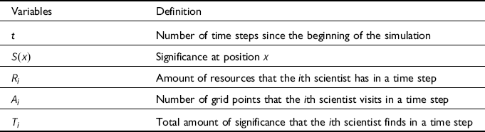
Parameters and variables are summarized in tables 1 and 2, respectively.
Summary of Parameters
| Parameters | Definition | Default Value |
|---|---|---|
 ${\mu _i}$ |
Position of the center of the ith Gaussian peak | — |
 ${h_i}$ |
Height of the ith Gaussian peak | 30 |
 ${\sigma _i}$ |
Width of the ith Gaussian peak | 4 |
 $\lambda $ |
Depletion rate of landscape | 0.9 |
| N | Total number of scientists on the landscape | 20 |
| d | Threshold for removal of scientists | 2 |
| q | Probability that a new scientist comes from other disciplines | — |
 ${R_T}$ |
Total amount of research resource | 50 |
| p | Proportion of resources for competitive selection | — |
 ${N_c}$ |
Number of scientists who receive competitive funding | 5 |
 ${N_n}$ |
Number of scientists who receive noncompetitive funding | — |
Summary of Variables
| Variables | Definition |
|---|---|
| t | Number of time steps since the beginning of the simulation |
 $S\left( x \right)$ |
Significance at position
 $x$ |
 ${R_i}$ |
Amount of resources that the ith scientist has in a time step |
 ${A_i}$ |
Number of grid points that the ith scientist visits in a time step |
 ${T_i}$ |
Total amount of significance that the ith scientist finds in a time step |
3.1.1. Landscape settings
An epistemic landscape of
 $101 \times 101$
grids is assumed. The initial significance of each grid is set by the summation of n Gaussian peaks. Because the actual research fields are too complex to be represented by a very smooth landscape, following Pöyhönen (Reference Pöyhönen2017), I introduce a small ruggedness into the landscape. Let
 ${{{\mu}_i}}$
,
 ${h_i}$
, and
 ${\sigma _i}$
be the center, height, and width of the ith Gaussian peak, respectively. Then, the initial significance of the position
 $x$
,
 $S\left({x} \right)$
, is set as
 $$S\left({x} \right) = \mathop \sum \limits_{i = 1}^n {h_i}{\rm{exp}}\left( { - {{|{{x}} - {{{{\mu}} _i}}{|^2}} \over {2\sigma _i^2}}} \right) + e,$$
where e is a random variable that obeys a uniform distribution within the interval
 $\left[ {0,1} \right]$
. As in Pöyhönen (Reference Pöyhönen2017), when a grid is visited by a scientist, the significance of the grid is reduced to
 $\left( {1 - \lambda } \right)S\left({x} \right)$
. However, throughout this study, it is assumed that
 $\lambda $
is so large (i.e.,
 $ = 0.9$
) that replications of previous studies have only a slight significance
Footnote 7
(note that
 $\lambda \lt 1$
prevents scientists from being trapped in local regions).
3.1.2. Settings for the scientists
Initially, N scientists are randomly located in the landscape. At each time step, they perform research by using the resources provided by the central funding agency. Let
 ${R_i}$
be the amount of resources that the ith scientist has in a focal time step (for the determination of
 ${R_i}$
, see following discussion). On average, a unit of resource is required to investigate each grid point, and scientists succeed in exploring a grid point at a rate proportional to the amount of resources. To represent this, the number of grid points that a scientist with resource
 ${R_i}$
visits in a time step,
 ${A_i}$
, is determined by the Poisson distribution with mean
 ${R_i}$
.
Footnote 8
All scientists are assumed to be hill-climbers, such that they move to the grid with the highest significance in the Moore neighborhood until
 ${A_i}$
grids are investigated. When a scientist visits a grid of significance
 $S\left( x \right)$
,
 $\lambda S\left( x \right)$
of significance is obtained. The total amount of significance that the ith scientist finds in a time step (i.e., their performance in the time step) is recorded as
 ${T_i}$
and is used to determine
 ${R_i}$
in the next time step (see following discussion).
The turnover of scientists occurs in such a way that inactive scientists are replaced by new scientists. When scientists do not conduct research (i.e.,
 ${A_i} = 0$
) in successive d time steps, they are removed from the landscape, and new scientists are introduced so that the total number of scientists is kept at N. A parameter q is introduced to represent the “openness” of the discipline to scientists from other disciplines. Thus, with probability q, a new scientist is assumed to come from other disciplines and have a research project that could be completely different from previous studies. In such cases, the initial position is assigned at random. Alternatively, with probability
 $1 - q$
, a new scientist is assumed to have come from one of the present laboratories in the discipline. In such cases, a scientist in the landscape is randomly chosen, and the new scientist is located in the same grid. In either case,
 ${T_i} = 0$
is initially assigned for new scientists. When
 $q = 1$
, new scientists always come from other disciplines and have novel research projects, as in Avin’s model.
3.1.3. Resource distribution
At every time step, the central funding agency distributes resources to the scientists in the landscape. The total amount of resources is fixed at
 ${R_T}$
for each time step. The proportion p of the resources is assigned by competition and distributed equally among scientists whose
 ${T_i}$
(i.e., performance in the previous round) is among the top
 ${N_c}$
. This distribution by competition is expected to work similarly to peer review (and the best-visible strategy in Avin’s model) because it tends to fund researchers investigating well-recognized topics.
Footnote 9
The remaining resources are distributed equally among
 ${N_n}$
scientists who win in the lottery system. Then, for those scientists whose
 ${T_i}$
is within the top
 ${N_c}$
,
 ${R_i}$
in the next time step is given by
 $${R_i} = \left\{ {\begin{array}{*{20}{c}}
{\frac{{p{R_T}}}{{{N_c}}} + \frac{{(1 - p){R_T}}}{{{N_n}}}} \hfill\;\;\;\;\; {({\rm{if\;win\;in\;the\;lottery, too}})} \\
{\frac{{p{R_T}}}{{{N_c}}}} \hfill\;\;\;\; {({\rm{otherwise}}).}\\
\end{array}} \right.$$
For others, it is given by
 $${R_i} = \left\{ {\begin{array}{*{20}{c}}
{\frac{{(1 - p){R_T}}}{{{N_n}}}} \hfill \;\;\;\;\; {({\rm{if\;win\;in\;the\;lottery}})} \hfill \\
0 \hfill \;\;\;\;\; {({\rm{otherwise}}).} \\
\end{array}} \right.$$
Various funding strategies can be represented by adjusting p and
 ${N_n}$
. p determines the proportion of resources distributed by competition.
 ${N_n}$
determines the chance of winning noncompetitive resource funding, such that a larger
 ${N_n}$
increases the chance of winning and, interchangeably, reduces the amount of resources allocated to each winner. When
 ${N_n} = N$
, a noncompetitive resource is allocated equally to all scientists (i.e., baseline funding). The funding distribution through competition only is realized by
 $p = 1$
. Funding only by lottery is realized by
 $p = 0$
and small
 ${N_n}$
, and funding only by baseline funding is realized by
 $p = 0$
and
 ${N_n} = N$
. A combination of these strategies is represented at intermediate values of p and
 ${N_n}$
.
3.2. Results
Extensive simulations were conducted to investigate the effect of various parameters on the efficiency of the scientific community, which is measured by the proportion of significance in the landscape found by scientists. To consider the best resource allocation strategy by a central funding agency, I focused mainly on two parameters:
p (ratio between competitive and noncompetitive funding) and
 ${N_n}$
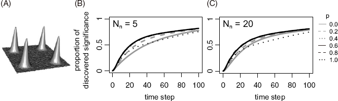
(chance of receiving noncompetitive funding). Throughout this section, the same initial landscape is used, as illustrated in figure 2A. For simplicity, the community size was fixed as
 $N = 20$
and the winning rate of the competitive funding at
 ${N_c} = 5$
to observe the effects of p and
 ${N_n}$
on the productivity of disciplines with various influx rates q. These assumptions do not affect the qualitative results presented (see appendix A).
(A) The initial shape of the landscape. (B and C) The proportion of significance found by scientists when
 $q = 1$
as a function of the number of time steps for (B)
 ${N_n} = 5$
and (C)
 ${N_n} = 20$
, respectively. The values were averaged over 1,000 replications.

3.2.1. A discipline with an extremely high influx rate
First, I consider a discipline with a very frequent interdisciplinary influx (i.e.,
 $q = 1$
), a situation similar to that in Avin’s model. The proportion of discovered significance is plotted with time while changing p for
 ${N_n} = 5$
(figure 2B) and
 ${N_n} = 20$
(figure 2C). The figure shows that the discovered significance is maximized for intermediate
 $p\sim0.6,0.8$
at all time points in both cases. Consistent with Avin’s model, this indicates that a combination of competitive and noncompetitive resource assignments is the most efficient. Also, in this case,
 ${N_n}$
(i.e., whether a noncompetitive grant is allocated by lottery or by baseline funding) does not significantly affect the efficiency.
The reason that intermediate p performs best can be understood by observing the dynamics of two extreme cases,
 $p\sim0$
and
 $p\sim1$
. As scientists with new research ideas continuously enter due to the assumption of a high q, scientists are distributed over the entire landscape. When p is very low, the resource is distributed mostly in a noncompetitive manner, and research activities are conducted in wide areas; thus, scientists tend to find all peaks at an early stage. However, due to the low p, this does not encourage the activities of scientists near the peaks, and the exploitation of the already-found peaks of significance is slow. On the other hand, when p is very high, the resource is distributed by competition, and scientific activities are conducted only in small areas around the already-found peaks. As a result, while the exploitation of the discovered peaks is very fast, the discovery of other peaks located far from the already-found peaks is slow. An optimal pattern is observed when p is intermediate, where exploration of new peaks and exploitation of already-found peaks are conducted in parallel. Noncompetitive resource allocation allows new scientists near unfounded peaks to be active, which promotes the early discovery of peaks. Once peaks are found, competitive funding promotes efficient exploitation of the peaks. The effect of
 ${N_n}$
is subtle, perhaps because any
 ${N_n}$
allows new scientists near peaks to initiate research and obtain further funding based on their achievements.
3.2.2. A discipline with an extremely low influx rate
Next, I consider a conventional discipline that scientists from other disciplines do not enter (i.e.,
 $q = 0$
). For the lottery distribution (
 ${N_n} = 5$
), shown in figure 3A, the proportion of discovered significance is plotted with time while changing p. This shows that a larger p is more effective for all time points. The reason for this pattern is revealed by the distribution of scientists in figure 4. Each white circle represents the position of each scientist, and its size represents the activity of the scientist in the preceding time step (i.e.,
 ${A_i}$
), whereas the background shade represents the significance landscape
 $S\left( x \right)$
. Because q is very low, new scientists always come from existing laboratories, and the turnover of scientists leads to the convergence of scientists’ positions. In fact, convergence is observed irrespective of p in figure 4. When p is very high, only those scientists close to the peaks survive for a long time and reproduce their descendants in the same grid around the peak. When p is very low, those who are lucky enough to keep winning the lottery can survive and reproduce their descendants in the same grid. However, in this case, their positions are not necessarily near the peaks. Thus, a larger p promotes the concentration of scientists around the peaks and improves their performance.
(A and B) The proportion of significance found by scientists when
 $q = 0$
as a function of the number of time steps for (A)
 ${N_n} = 5$
and (B)
 ${N_n} = 20$
. The values are averaged over 1,000 replications. (C) The difference between two cases (the case of
 ${N_n} = 20$
minus the case of
 ${N_n} = 5$
).

Typical simulation runs for
 $q = 0$
and
 ${N_n} = 5$
are shown for three values of p: (A)
 $p = 0.0$
, (B)
 $p = 0.4$
, and (C)
 $p = 1.0$
. Each white circle represents the position of a scientist, and its size represents
 ${A_i}$
in the preceding time step. The background shade shows the significance landscape
 $S\left( x \right)$
.

The pattern changes significantly in the case of equal distribution (i.e.,
 ${N_n} = 20$
). In figure 3B, the proportion of discovered significance is plotted with time for various p. In the short term, a relatively large
 $p \approx 0.6,0.8$
maximizes the findings. However, in the long run, a relatively small
 $p \approx 0.2,0.4$
yields the best performance.
To inspect the effect of
 ${N_n}$
on the community’s performance, the difference in performance between the noncompetitive resources distributed by lottery (
 ${N_n} = 5$
) and by baseline funding (
 ${N_n} = 20$
) was calculated (figure 3C). This shows that baseline funding works significantly better for all p unless the performance is evaluated in a very short run. Note that the two lines for
 $p = 1$
in figures 3A and 3B are identical because all the resources are distributed by competition, and the values of
 ${N_n}$
make no difference.
To explore the reason for this result, the distribution of scientists in typical simulation runs for
 ${N_n} = 20$
is shown in figure 5. As noted earlier, when p is very large (figure 5C), scientists aggregate in the same manner as in the case of
 ${N_n} = 5$
and
 $p\sim1$
. However, when p is very small, a great diversity of research projects is realized because, unlike the lottery case, continuous resource allocation allows all scientists to conduct research constantly, and turnovers are significantly reduced (figure 5A). Although diversity ensures that all peaks are found in a relatively short time, resource allocation to scientists at a less significant position slows the exploitation of the peak. A more efficient pattern is observed when p takes intermediate values (figure 5B). In this case, diversity is maintained by an equal resource allocation, whereas the exploitation of the peaks is enhanced by competitive resource allocation. The balance between exploration and exploitation makes intermediate p optimal for both short and long runs.
Typical simulation runs for
 $q = 0$
and
 ${N_n} = 20$
are shown for three p: (A)
 $p = 0.0$
, (B)
 $p = 0.4$
, and (C)
 $p = 1.0$
. Each white circle represents the position of a scientist, and its size represents
 ${A_i}$
in the preceding time step. The background shade shows the significance landscape
 $S\left( x \right)$
.

These results suggest that an equal distribution of resources outperforms random distribution because the equal distribution leads to a lower turnover rate of scientists compared to that in the distribution by lottery. To investigate whether the lower turnover rate in the equal distribution is generally observed (i.e., outside the parameter spaces investigated), I calculated the expected time until a new scientist at a region of very low significance is replaced under simplified situations. To focus on scientists in a region of low significance, it is assumed that a focal scientist does not win a competitive grant and relies solely on noncompetitive resources. Then, the expected time until the replacement,
 $\tau $
, is given by
 $$\begin{array}{l}
\tau = \frac{{\sum\nolimits_{i = 0}^{i = d - 1} {{\alpha ^i}} }}{{{\alpha ^d}}} \\
= \left\{ {\begin{array}{*{20}{c}}
d \hfill \;\;\;\;{{\rm{for }}\;\;\;\;\alpha {\rm{ = 1}}} \\
{\frac{{1 - {\alpha ^d}}}{{{\alpha ^d}(1 - \alpha )}}} \hfill \;\;\;{{\rm{for }}\;\;\;\alpha \ne {\rm{1,}}} \\
\end{array}} \right. \\
\end{array}$$
where
 $\alpha = \left( {1 - {{{N_n}} \over N}} \right) + {{{N_n}} \over N}{\rm{exp}}\left( { - {{\left( {1 - p} \right){R_T}} \over {{N_n}}}} \right)$
. It can be deduced that
 $\tau $
is a monotonically increasing function with respect to
 ${N_n}$
. In other words, the turnover becomes less frequent as
 ${N_n}$
increases for all combinations of
 $p,{R_T},N$
, and d (for details of the derivations, see appendix B).
To visualize the effect of
 ${N_n}$
, equation (4) is plotted for various p and
 ${N_n}$
(figure 6). When
 ${N_n}$
is low,
 $\tau $
is so small that scientists in a valley of significance are likely to be replaced before reaching another peak of significance, irrespective of p. On the other hand, when
 ${N_n}$
is very large, scientists in a region of low significance can survive for enough time to find new peaks, especially for low p. These results suggest that in a discipline with a low influx rate, equal distribution of noncompetitive resources is superior to random distribution.
The expected time until a new scientist at a region of low significance is replaced,
 $\tau $
, is plotted for various p and
 ${N_n}$
. The other parameters are set at default values (see table 1).

Note that these mathematical analyses do not depend on any assumptions about the shape of the landscape, such as its dimensions, size, and the location of peaks. Thus, these results would hold for a wide class of landscapes.
3.2.3. A discipline with intermediate influx rates
Finally, I consider cases for intermediate values of q (
 $0 \lt q \lt 1$
). To see how the performance and optimal p change for both the random distribution (i.e.,
 $N_n = 5$
) and the equal distribution (i.e.,
 ${N_n} = 20$
), the performance of the community for each set of (
 $p,q$
) is evaluated, where p and q are increased by 0.01. For each parameter set, 1,000 replications of simulations were run, and the average of discovered significance was calculated at
 $t = 50$
. Then, for each q, an optimal value of p was estimated. The performance for the optimum p is plotted along with q for both distribution methods in figure 7A. The equal distribution (gray line) shows a similar or better performance than the random distribution (black line). Notably, the equal distribution significantly outperforms the random distribution for
 $q \lt 0.2$
. For
 $q \gt 0.2$
, the random distribution performs slightly better; however, both methods show similar performances. Considering that it is unclear whether we can identify the influx rate of a given discipline, this result suggests that equal distribution is a better choice.
(A) The performance using optimal p is plotted against q for
 ${N_n} = 5$
(black line) and
 ${N_n} = 20$
(gray line). The performance is defined as the average of discovered significance at
 $t = 50$
. (B) The optimum value of p is plotted against q for
 ${N_n} = 5$
(black line) and
 ${N_n} = 20$
(gray line).

The optimal values of p are plotted in figure 7B. For
 ${N_n} = 20$
, the optimal p monotonically increases with q because the need to reduce the turnover rate declines as the diversity of research projects is maintained by new scientists. For
 ${N_n} = 5$
, the optimal p is reduced from 1 to
 $\sim0.5$
around
 $q \approx 0.05$
because a continuous influx of new research ideas increases the benefit of noncompetitive resource allocation. For larger q, dynamics similar to the case of
 ${N_n} = 20$
are observed. These results show that even in intermediate q, the performance of the community and the optimal value of p are affected by the way noncompetitive resources are distributed and that, overall, a combination of competitive and equal distribution is a better choice.
Footnote 10
4. Discussion
The presented results show that baseline funding performs better or similarly in many situations when compared with lottery funding. This trend is seen in a wide range of parameter settings (see appendices A and D) and is also supported by general mathematical analysis. Thus, considering our insufficient knowledge about the parameters, baseline funding would be a better option than lottery funding as a general funding strategy. Because baseline funding is easy to implement, it is preferable from the perspective of cost performance (see appendix E for ideas on how to explicitly incorporate implementation costs into the model).
The model also shows that a combination of competitive and noncompetitive distributions is often optimal. In general, the optimal proportion of competitive funding increases as scientists’ interdisciplinary movement increases. The optimal proportion also depends on other parameters, such as the shape of the landscape (see appendix A). These results suggest that funding agencies should change the proportion of competitive and noncompetitive funding for different disciplines.
At this point, one may question the utility of the landscape approach for actual policy making. Landscape models simplify many aspects of a complex research community. Furthermore, currently, we do not have deep knowledge about the parameters in the model, such as the shape of the landscape and the extent of interdisciplinary mobility. Given these limitations, one may doubt the usefulness of landscape models in discussing actual scientific communities. Footnote 11
However, I argue that the conclusion of the present study—that is, that baseline funding is a better general strategy than lottery funding—has substantial generality. First, as discussed in section 3, the assumption of a smooth landscape is not unrealistic. Second, the conclusion does not depend on specific assumptions regarding parameter values, and it covers a wide range of parameter spaces. This generality provides a strong reason to expect that the same conclusion would be applicable to the actual community.
The current model can be extended in various ways to make it more realistic (see appendix E for other ideas for extensions). For instance, in the present model, the expected activity of the ith scientist (
 ${A_i}$
) is assumed to be proportional to the amount of resources (
 ${R_i}$
). This means that the manner in which resources are distributed does not affect the total amount of activity (i.e., the total number of grids investigated in a time step in a discipline). However, it is likely that a very small amount of funds would not allow for any research activity. In such cases, equal distribution among many scientists would be ineffective. In addition, we could impose an upper limit on a researcher’s amount of activity in a time step irrespective of their resources. Recent studies have revealed that research performance is maximized at intermediate grant sizes (for a review, see Aagaard et al. [Reference Aagaard, Kladakis and Nielsen2020]). Given that the current funding systems tend to overly concentrate resources on a small number of scientists (Wahls Reference Wahls2018; Aagaard et al. Reference Aagaard, Kladakis and Nielsen2020), an equal distribution may be beneficial from the perspective of efficient use of funding resources (see also Vaesen and Katzav [Reference Vaesen and Katzav2017]).
Another important assumption in the current model is that scientists’ ability to conduct research is equal, but this may not be the case. Although one may worry that the incorporation of such aspects would require evaluation of scientists’ ability and return to the peer-review system, there are ways in which noncompetitive funding could also incorporate such an evaluation. For example, the incorporation of some prescreening processes might be effective in excluding poor-quality proposals or pseudo-scientific ones, such as the approach implemented by the Health Research Council of New Zealand. Additionally, minimum quality control may be possible at earlier stages, such as during education or at the time of employment in research institutions.
Recently, empirical data on the evolution of the scientific community have become accessible (for a review, see Fortunato et al. [Reference Fortunato, Bergstrom, Katy Börner, Evans, Milojević, Petersen, Radicchi, Sinatra, Uzzi, Vespignani, Waltman, Wang and Barabási2018]), leading to evidence-based policy making. Theoretical analyses should work in a complementary manner to those empirical studies in policy making. With the accumulation of empirical evidence, more realistic models can be developed. Such models would be useful for studying the dependence of the effectiveness of policies on certain parameters, helping to test the generality of the expected effects of those policies. In turn, this would also help identify some important parameters, stimulating further empirical research on these parameters. The strength of the present model is its flexibility, which allows various types of extensions to better represent the actual dynamics of science (see appendix E). Thus, the current model provides a useful theoretical framework for future studies.
5. Conclusion
Recently, research funding systems have undergone significant reforms, and many new methods of funding distribution have been introduced (Larrue et al. Reference Larrue, Guellec and Sgard2018). One such method is funding distribution by lottery, which was first introduced by the Health Research Council of New Zealand. A rationale for this method is that a lottery system inherently imposes no systematic bias, whereas conventional peer review introduces a bias against the innovative approach, which could slow down scientific progress in the long run (Brezis Reference Brezis2007; Gillies Reference Gillies2014; Fang and Casadevall Reference Fang and Casadevall2016).
Avin’s work (Reference Avin, Mäki, Votsis and Ruphy2015, Reference Avin2019a) was among the first to address this problem and examine the effectiveness of various funding strategies of a central funding agency. He extended the epistemic landscape model and argued that a combination of competitive funding, such as the peer-review process, and noncompetitive funding by lottery is the best funding strategy. However, his model missed two important aspects: (i) noncompetitive funding distributed equally among scientists, such as block grants, and (ii) realistic interdisciplinary dynamics of scientists.
To resolve this problem, I extended the epistemic landscape model to consider more general situations. This model was used to investigate the importance of these two missing aspects, and it was found that they significantly affected the optimal funding strategy. Although a combination of lottery and competitive distribution is recommended in Avin’s studies, the current model shows that when most new scientists come from the same discipline, a combination of baseline funding, such as block grants, and competitive funding works better. When new scientists frequently come from other disciplines, both methods work with similar efficiency. These results validate that a combination of competitive and noncompetitive distribution is an optimal strategy and suggest that, as a method of noncompetitive distribution, baseline funding is a better choice than funding by lottery in many cases.
For simplicity, and owing to the lack of empirical data, several assumptions were made in the model. Although they could affect the quantitative dynamics of the proposed model, I expect that the qualitative pattern would remain robust against these assumptions, considering that similar patterns are observed over a wide range of parameter spaces. An advantage of the current model is its flexibility to allow further sophistication. When empirical studies accumulate, future work may incorporate this information into the model and predict the dynamics of an actual community more accurately.
Acknowledgments
This manuscript is based on a science and society subthesis submitted to SOKENDAI (Graduate University for Advanced Studies). I am grateful to my supervisor Yukinori Onishi for helpful discussions and comments on this manuscript. I would also like to thank two anonymous reviewers for their insightful comments. This work is partly supported by SOKENDAI. Codes used for simulations are available at https://github.com/TSakamoto-evo/funding.
Appendix A: Dynamics in Other Parameters
The effects of the shape of the landscape and the parameter
 ${N_c}$
were investigated to check the generality of the conclusions presented in the main text. Qualitatively similar dynamics were observed here.
First, the effects of the landscape shape were investigated. Three different peak widths (i.e.,
 $\sigma $
) are assumed in figure S1. Consistent with the results presented in the main text, equal funding distribution outperforms random distribution when
 $q$
is small. The advantage decreases as
 $\sigma $
increases (figure S1, panels B, E, and H) because a small valley of significance reduces the need to support scientists who are crossing the valley. For the same reason, increasing competitive funding is more beneficial as
 $\sigma $
increases (figure S1, panels C, F, and I). When
 $q$
is large, the two distribution methods of noncompetitive funding show similar performance for the three cases. The effect of the number of peaks was also considered. Three different numbers of peaks are assumed in figure S2. The qualitative results are very similar for the three cases. In summary, the shape of the landscape does not significantly affect the quantitative results.
The investigated landscape, the performance of the scientific community, and the optimal
 $p$
are plotted for (A–C)
 $\sigma = 4.0$
, (D–F)
 $\sigma = 7.0$
, and (G–I)
 $\sigma = 10.0$
, respectively. All parameters except for
 $\sigma $
are the same as that in figure 7, so panels B and C are identical to figures 7A and 7B, respectively.

The investigated landscape, the performance of the scientific community, and the optimal
 $p$
are plotted for (A–C) two peaks, (D–F) four peaks, and (G–I) six peaks, respectively. All parameters except for the number of peaks are the same as those in figure 7, so panels E and F are identical to figures 7A and 7B, respectively.

Next, the effects of parameter
 ${N_c}$
were investigated.
 ${N_c}$
is the parameter that determines the acceptance rate of competitive funding. Two different
 ${N_c}$
values are shown in figure S3. Regarding the shape of the landscape,
 ${N_c}$
does not affect the qualitative results.


Appendix B: Derivation of Equation (4)
Here, a detailed derivation of equation (4) is provided. Proofs for the statements referred to in the main text are also included.
The probability that no activity is conducted in a time step: Recall that the number of activities conducted in a time step,
 ${A_i}$
, obeys a Poisson distribution with mean
 ${R_i}$
, where
 ${R_i}$
is given by equation (S8). The probability that no activity is conducted in a time step,
 $\alpha $
, is represented by
 $$\alpha = \left( {1 - {{{N_n}} \over N}} \right) + {{{N_n}} \over N}{\rm{exp}}\left( { - {{\left( {1 - p} \right){R_T}} \over {{N_n}}}} \right).$$
Corollary:
 $\alpha $
decreases as
 ${N_n}$
increases. The derivative of
 $\alpha $
with respect to
 ${N_n}$
is
 $${{d\alpha } \over {d{N_n}}} = {{{e^{ - a/{N_n}}}} \over N}\left( {1 + {a \over {{N_n}}} - {e^{a/{N_n}}}} \right),$$
where
 $a = \left( {1 - p} \right){R_T} \geqslant 0$
. Note that
 $a = 0$
only when
 $p = 1$
. Let
 $f\left( {{N_n}} \right) = 1 + {a \over {{N_n}}} - {e^{a/{N_n}}}$
. Then,
 $f'\left( {{N_n}} \right) = {a \over {N_n^2}}\left( {{e^{a/{N_n}}} - 1} \right) \ge 0$
, and
 $f\left( { + \infty } \right) = 0$
, resulting in
 $f\left( {{N_n}} \right) \le 0$
for
 ${N_n} \gt 0$
. From equation (S2), it is clear that
 $\alpha $
is a monotonically decreasing function with respect to
 ${N_n}$
. Specifically, when
 $p \lt 1$
,
 $\alpha $
is a strictly decreasing function with respect to
 ${N_n}$
.
Derivation for equation (
4
): Let
 ${T_i}$
(
 $i \in \left\{ {0,1,2, \cdots ,d - 1} \right\}$
) be the expected time until replacement when a scientist fails to conduct research in
 $i$
successive time steps in the initial state. By considering the fate in the next time step, the following recursions are derived:
 $${T_i} = \left\{ {\matrix{ {1 + \alpha {T_{i + 1}} + \left( {1 - \alpha } \right){T_0}} \hfill & {\left( {0 \le i \le d - 2} \right)} \hfill \cr {1 + \left( {1 - \alpha } \right){T_0}} \hfill & {\left( {i = d - 1} \right).} \hfill \cr } } \right.$$
From equation (S3), it is deduced that
 $${T_{i + 1}} - {T_i} = \left\{ {\matrix{ {\alpha \left( {{T_{i + 2}} - {T_{i + 1}}} \right)} \hfill & {\left( {0 \le i \le d - 3} \right)} \hfill \cr { - \alpha {T_{i + 1}}} \hfill & {\left( {i = d - 2} \right).} \hfill \cr } } \right.$$
Then,
 ${T_{i + 1}} - {T_i} = - {\alpha ^{d - i - 1}}{T_{d - 1}}$
. From this equation,
 ${T_0}$
is expressed as
 $$\matrix{ {{T_0}} \hfill & { = {T_{d - 1}} - \mathop \sum \limits_{i = 0}^{i = d - 2} {\rm{}}({T_{i + 1}} - {T_i})} \hfill \cr \hfill & { = {T_{d - 1}}\mathop \sum \limits_{i = 0}^{i = d - 1} {\rm{}}{\alpha ^i}.} \hfill \cr } $$
By substituting equation (S5) into equation (S3) for
 $i = d - 1$
,
 ${T_{d - 1}} = {1 \over {{\alpha ^d}}}$
is obtained. By noting that
 $\tau = {T_0}$
and substituting it into equation (S5), equation (4) is derived.
Corollary:
 $\tau $
decreases as
 $\alpha $
increases. The derivative of
 $\tau $
with respect to
 $\alpha $
is
 $${{d\tau } \over {d\alpha }} = {{{\alpha ^{ - d - 1}}} \over {{{(\alpha - 1)}^2}}}g\left( \alpha \right),$$
where
 $g\left( \alpha \right) = d\left( {\alpha - 1} \right) - \alpha \left( {{\alpha ^d} - 1} \right)$
. Because
 $g'\left( \alpha \right) = \left( {d + 1} \right)\left( {1 - {\alpha ^d}} \right) \geqslant 0$
and
 $g\left( 1 \right) = 0$
,
 $g\left( \alpha \right) \le 0$
for all
 $\alpha \lt 1$
. Then, it is shown that
 $\tau $
is a monotonically decreasing function with respect to
 $\alpha $
. Note that
 $\alpha = 1$
only when
 $p = 1$
(see equation [S1]), and when
 $p \lt 1$
,
 $\tau $
is a strictly decreasing function.
It is demonstrated that
 $\tau $
decreases as
 $\alpha $
increases while
 $\alpha $
decreases as
 ${N_n}$
increases. By integrating these, it is shown that
 $\tau $
increases as
 ${N_n}$
increases.
Appendix C: Coexistence of Baseline Funding and Lottery
In this section, I consider a case where the coexistence of baseline funding and funding by lottery is allowed. The details of the implementation are as follows. Let
 ${p_c}$
and
 ${p_l}$
(
 ${p_c} + {p_l} \le 1$
) be the proportion of resources assigned by competitive method and lottery, respectively. The remaining proportion of
 $1 - {p_c} - {p_l}$
is granted resources by baseline funding. I denote by
 ${N_l}$
the number of scientists who win a lottery. Accordingly, equations (2) and (3) are modified as follows. For those who win via competitive funding,
 $${R_i} = \left\{ {\matrix{ {{{{p_c}{R_T}} \over {{N_c}}} + {{{p_l}{R_T}} \over {{N_l}}} + {{\left( {1 - {p_c} - {p_l}} \right){R_T}} \over N}} \hfill & {\left( {{\rm{if\;\;win\;\;in\;\;the\;lottery}},{\rm{\;\;too}}} \right)} \hfill \cr {{{{p_c}{R_T}} \over {{N_c}}} + {{\left( {1 - {p_c} - {p_l}} \right){R_T}} \over N}} \hfill & {\left( {{\rm{otherwise}}} \right).} \hfill \cr } } \right.$$
For others,
 $${R_i} = \left\{ {\matrix{ {{{{p_l}{R_T}} \over {{N_l}}} + {{\left( {1 - {p_c} - {p_l}} \right){R_T}} \over N}} \hfill & {\left( {{\rm{if\;\;win\;in\;\;the\;lottery}}} \right)} \hfill \cr {{{\left( {1 - {p_c} - {p_l}} \right){R_T}} \over N}} \hfill & {\left( {{\rm{otherwise}}} \right).} \hfill \cr } } \right.$$
Using this model, I investigated the optimal funding strategy (
 ${p_c}$
and
 ${p_l}$
) for various
 $q$
. Consistent with the main study, I assumed
 ${N_c} = {N_l} = 5$
. For each
 $q$
,
 ${p_c}$
and
 ${p_l}$
were increased by 0.01, and the optimal combination was identified. Figure S4 shows that at the optimal combination, either
 ${p_l}$
or
 $1 - {p_c} - {p_l}$
is generally
 $\sim 0$
, and the performance at the optimum is almost equal to the maximum of the performance of the two cases in figure 7. These results suggest that baseline funding and funding by lottery are optimally exclusive.
(A) The performance of the optimal p c and p i at the optimum is plotted against q (bold line). The performance is defined as the average of discovered significance at t = 50. For comparison, the two lines in figure 7 are also drawn in thin lines. (B) The optimum proportion of resources for each funding method is plotted against q.

Appendix D: Effect of Initial Distribution of Scientists
In this section, the effect of scientists’ distribution at the initial state is considered. In the main text, a random distribution is assumed because it is simple and consistent with previous studies (Avin Reference Avin, Mäki, Votsis and Ruphy2015, Reference Adam2019a). Such a random distribution may be appropriate for representing the initial state of new disciplines, where most researchers come from other disciplines. However, the distribution may not be random if a focal discipline has some history before the consideration of the current funding distribution. In that case, the initial distribution of scientists may be affected by the manner in which the discipline has evolved. Footnote 1 To investigate such an effect, I constructed a slightly different simulation model in which the effect of the funding method on scientists’ distribution is explicitly taken into account.
In this new model, I assume that a new peak of significance arises at a random position when the total remaining significance is less than
 ${S_c}$
(
 ${S_c} = 5,000$
is assumed). A similar situation was considered by Avin (Reference Adam2019a) for the “new avenues” setting. Such an assumption enables the discipline to evolve for a long time without exhausting significance. After evolving for 1,000 time steps, the scientists’ distribution would no longer depend on the initial distribution. I then calculated the speed of discovery of significance in the following 10,000 time steps. Using this model, I increased
 $p$
and
 $q$
by 0.01 for both baseline funding and lottery and registered their performances.
Despite the large difference in the model setting, roughly similar patterns are observed in this model: baseline funding is better than lottery funding when
 $q$
is small and slightly worse when
 $q$
is relatively large. The performance (discovered significance per time step) of each (
 $p,q$
) set is shown by the shaded colors in figure S5A. The black line represents the optimal
 $p$
for each
 $q$
. This demonstrates that the performance of lottery funding is worse than that of baseline funding when
 $q$
is small (i.e.,
 $ \lt 0.1$
), whereas lottery is slightly better when
 $q$
is relatively large (i.e.,
 $ \gt 0.2$
). I also plotted the performance of each funding method when
 $p$
is optimal (in) figure S5B), in a manner similar to that of figure 7A, and observed a similar trend.
Footnote 2
Performance of the scientific community. (A) Performance at each (p, q) for the lottery (Nn = 5) and baseline (Nn = 20) cases. Shaded colors represent the performance, and the black line shows the optimal p for each q. (B) Performance at optimal p. (C) Proportion of performance change after baseline funding is replaced with funding by lottery.

To compare the performance of the two methods in more detail, I plotted the proportion of the performance change for some sets of (
 $p,q$
) when baseline funding is replaced with lottery (figure S5C). When
 $q$
is small, the switch from baseline funding to lottery funding decreases the performance for all
 $p$
. The reduction can be as large as
 $ \gt 50\% $
when
 $p$
is small. When
 $q$
is large, the performance increases for some
 $p$
, but the increment is relatively small (
 $\!\!\lt 15\% $
). Because our current knowledge about
 $q$
is insufficient, this result seems to suggest that baseline funding is a better choice than lottery funding as a general policy.
Appendix E: Various Potential Extensions of the Model
In this section, I discuss how various factors, such as the ability of scientists, the efficiency of resources, and the different costs among the funding methods, could be incorporated into the present model.
The varying abilities of scientists can be implemented in several ways. Let
 ${c_i}$
be the ability of
 $i$
th scientist. If we want to represent the varying speed of excavating each research topic (i.e., grid point) among scientists, it may be realized by determining
 ${A_i}$
using a Poisson distribution with mean
 ${c_i}{R_i}$
, rather than
 ${R_i}$
. If we want to incorporate the varying skills in writing grant applications, it may be introduced in a way that competitive resources are distributed based on
 ${c_i}{T_i}$
, rather than
 ${T_i}$
.
The varying efficiency of resources can be implemented as follows. We first consider the case in which the expected activity per unit resource depends on the total amount of resources of a scientist. If such dependency is given by a function
 $f\left( R \right)$
,
 ${A_i}$
may be determined by the Poisson distribution with mean
 ${R_i}f\left( {{R_i}} \right)$
. Instead, we can represent that each grid point differs in the difficulty of the investigation, such that some grid points require many resources for success. Let
 $\gamma \left({x} \right)$
be the difficulty of investigating a grid point at position
 ${x}$
. Then, the
 $i$
th scientist with resource
 ${R_i}$
may take time
 $z$
to investigate the focal grid point, where
 $z$
is drawn from an exponential distribution with mean
 $\gamma \left( \bf{x} \right)/{R_i}$
.Footnote 3 In each time step, the
 $i$
th scientist is allowed to move as long as the sum of
 $z$
in that time step is less than 1. When
 $\gamma \left({x} \right) \equiv 1$
, this implementation is mathematically identical to that in the main text. Note that actual scientists may not be hill-climbers of significance in this case because they may also take
 $\gamma \left({x} \right)$
into account when choosing the next grid point.
Finally, the cost of implementing each funding method can be calculated as follows. In reality, different funding methods would require different costs for their implementation.
Footnote 4
Such implementation costs can be represented by reducing the amount of resources distributed by each method. For example, if the implementation of peer review requires the resource
 ${c_p}$
, the amount of resource that is distributed to grant winners may be
 $${{p{R_T} - {c_p}} \over {{N_c}}}$$
. Similar extensions can be considered for other funding methods. Instead, if we want to consider the cost of scientists spending time in preparation or review of application documents, it can be modeled such that
 ${A_i}$
is determined by a Poisson distribution with a mean
 $\left( {1 - {c_p}} \right){R_i}$
, where
 ${c_p}$
is the proportion of time each scientist invests in such activities.