Implications
Benefits that mixed crop–livestock systems take over specialized systems are controversial. Whereas previous studies mainly focused on the effect of crop–livestock interactions, we highlight here that crop–livestock organization (% crop–livestock) also is a main factor influencing the economic, environmental and production performances of mixed crop–livestock systems. As a consequence, we recommend using typologies of MC–L systems considering not only crop–livestock interactions but also crop–livestock organization to identify the set of farming practices that permits reaching the best compromise between sustainability objectives.
Introduction
In the past half-century, global intensification and specialization of agriculture is observed, mainly in developed regions as Europe (Peyraud et al., Reference Peyraud, Taboada and Delaby2014), United Kingdom (Wilkins, Reference Wilkins2008), or North America (Russelle et al., Reference Russelle, Entz and Franzluebbers2007). However, this specialization of territories and farming systems is widely criticized. On one side, this specialization has shown limits in terms of environmental performances. For instance, specialization of territories has led to a loss of biodiversity in comparison with diversified territories (i.e. with crop and livestock productions) (Lemaire, Reference Lemaire2007; Tichit et al., Reference Tichit, Puillet, Sabatier and Teillard2011). Furthermore, the specialization process in favor of crop production led to an abandonment of permanent pasture, preventing carbon sequestration (Soussana and Lemaire, Reference Soussana and Lemaire2014). In the same way, at the farming system scale, it has been proven that the non-renewable energy consumption increases when crop–livestock interactions are not optimized (Benoit and Laignel, Reference Benoit and Laignel2010). On the other side, economic performances of specialized systems on the long run are also criticized. Indeed, specialized farming systems are highly dependent on input markets. As a consequence, even if economies of scale (i.e. the economic gains due to an increase in production scale) still drive specialization of farming systems in developed countries, those systems are liable to struggle to maintain good profitability in front of the expected higher volatility of market prices (Bell and Moore, Reference Bell and Moore2012; Bommarco et al., Reference Bommarco, Kleijn and Potts2013).
For all these above mentioned reasons, mixed crop–livestock (MC–L) systems are claimed more sustainable than specialized farming systems regarding economic and environmental performances on the long run. These potential gains are tied to the concept of crop and livestock integration, itself tied to the concept of economies of scope. Economies of scope occur when a farm that produces two (or more) different products can get higher average output volumes or lower average production costs than two (or more) separate farms each selling just one product (at a constant amount of factors of production). The ability of MC–L systems to produce food while providing ecosystem services, facing climate change and volatility of commodity and input prices yet has been widely highlighted (Bonaudo et al., Reference Bonaudo, Bendahan, Sabatier, Ryschawy, Bellon, Leger, Magda and Tichit2014; Lemaire et al., Reference Lemaire, Franzluebbers, Carvalho and Dedieu2014; Peyraud et al., Reference Peyraud, Taboada and Delaby2014). However, we found quantitative scientific studies showing opposite socio-economic and/or environmental effects of crop–livestock interactions (Perrot et al. Reference Perrot, Caillaud and Chambaut2012; Ryschawy et al., Reference Ryschawy, Choisis, Choisis, Joannon and Gibon2012; Veysset et al., Reference Veysset, Lherm, Bebin and Roulenc2014). Those results consolidates the calls for better understanding the effects of crop–livestock interactions at farm scale (Parsons et al., Reference Parsons, Nicholson, Blake, Ketterings, Ramírez-Aviles, Cherney and Fox2011a).
Those contrasted results on the economic and environmental advantages of mixed crop–livestock system can be partly explained by two main reasons mentioned in the literature. First, studies mainly focus on the impact of crop–livestock interactions at a given biophysical process level (i.e. the soil fertility, the farm plot, etc.) without considering the impacts at farm scale (Russelle et al., Reference Russelle, Entz and Franzluebbers2007; Wilkins, Reference Wilkins2008). Second, at farm scale, results are affected by the complex interactions between subsystems and are highly dependent on the context of production (Bell and Moore, Reference Bell and Moore2012; Bell et al., Reference Bell, Moore and Kirkegaard2014). In this paper, we posit that those contrasted results on the advantages that MC–L systems may take over specialized systems are mainly due to the lack of production scale concerns when comparing farming systems. Indeed, while some studies completely fails to consider the production scale in their comparisons (Parsons et al., Reference Parsons, Nicholson, Blake, Ketterings, Ramírez-Aviles, Fox, Tedeschi and Cherney2011b; Ryschawy et al., Reference Ryschawy, Choisis, Choisis, Joannon and Gibon2012; Veysset et al., Reference Veysset, Lherm, Bebin and Roulenc2014), others take into account both scale economies and scope economies (Morrison et al., Reference Morrison, Kingwell and Pannell1986; Kingwell and Pannell, Reference Kingwell and Pannell1987; Perrot et al., Reference Perrot, Caillaud and Chambaut2012). However, those last studies – focusing on economic gains or losses – fail considering the effects on environmental and production performances whereas these are crucial objectives for sustainable production. Furthermore, those studies do not explore the links between scale and scope economies, that is the impacts of crop and livestock production scales on the capacity of the farming system to benefit from scope economies.
In this paper, to better take into account those effects, we defined the concept of crop–livestock organization as the percentage of the total agricultural area that is dedicated to crop and pasture production. We then argue that the crop–livestock organization has a direct and an indirect impact on mixed crop–livestock systems sustainability (mainly economic and environmental). The direct effect of crop–livestock organization is studied by comparing the performances of two MC–L systems with contrasted crop–livestock organizations (MC20–L80: mixed crop–livestock system with 20% of crops; MC80–L20: 80% of crops) and without crop–livestock interactions. The indirect effect of crop–livestock organization is analyzed through the comparison of the capacity of the same two contrasted MC–L systems to enhance their performances through crop–livestock interactions. The concepts of direct and indirect effects permit analyzing crop–livestock integration – which is usually only studied from the crop–livestock interactions viewpoint – from the crop–livestock organization viewpoint. Those concepts should not be confused with the concepts of direct and indirect interactions introduced by Moraine et al. (Reference Moraine, Duru, Nicholas, Leterme and Therond2014), which distinguish the interactions that occur in space and those that correspond to flows of materials or energy respectively. In this study, we consider both types of interactions but without distinguishing them given our aim to focus on better understanding the direct and indirect effects of crop–livestock organization. To analyze those effects, a model-based exploration methodology is used to permit simulating contrasted farming practices while keeping a constant production context (Rossing et al., Reference Rossing, Meynard and Van Ittersum1997; Sterk et al., Reference Sterk, Van Ittersum, Leeuwis and Wijnands2007).
Next subsections explain first the generic model – that is which can be parameterized for various regions – that we build to test the impacts of crop–livestock organization on MC–L systems sustainability. Then, we describe its application on the case of French sheep-for-meat farming in France. After providing some insights about the impact of crop–livestock organization on economic, production and environmental performances of MC–L systems, we present the main issues that arose from our analysis.
Material and methods
We build a generic mixed crop–livestock model to test if crop–livestock organization has a direct and an indirect effect on the economic, production and environmental performances of MC–L systems. We first describe the key components of the model and the subsequent performance indicators generated. Then, we outline its parametrization on the specific case of French sheep-for-meat production in a typical fertile lowland area of France in the Vienne region. This area was chosen because of its relevance regarding our research study; almost all the agriculture area is arable and could be ploughed. Indeed, sheep-for-meat production in the Vienne has declined by 60% over the period 1989–2012 in favor of crop production, that is twice as fast as the national average (Agreste, 2013). Understanding conditions of mixing crop and sheep productions in that region is thus a key concern in that area. The simulation patterns conducted to analyze and better understand those conditions are described in the last subsection.
General model description
We built a mixed crop–livestock model applied to sheep-for-meat production – Sheep‘n’Crop – that permits simulating contrasted interactions between a vegetal and a livestock subsystem as well as their associated economic and environmental performances at farm scale. Sheep‘n’Crop is a whole-farm mathematical programming model that selects the annual gross margin-maximizing set of farm activities from various management options and constraints. For each set of farm activities selected, the capital (buildings and materials) and the quantity of labor needed are estimated to allow for a detailed quantification of the associated economic and environmental performances.
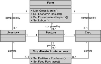
There are three categories of farm activities allowed: livestock production, pasture production and crop production (Figure 1). A livestock production obligatory implies an on-farm pasture production. At the opposite, crop and livestock productions are independent choices. When both crop and livestock productions are selected, various interactions may be (or not) selected to maximize the gross margin by reducing fertilizers and feed costs. Those interactions are allowed through farming activities as (i) feeding livestock by crop production, (ii) rotational patterns with pasture or intercrops, (iii) spreading manure on crops.
Class diagram (in Unified Modeling Language (UML)) illustrating the Sheep‘n’Crop model. A farm is composed by 0 or 1 livestock/pasture/crop subsystems. A livestock subsystem implicitly needs a pasture subsystem. All subsystems may or may not interact through a crop–livestock interactions subsystem.

Objective function
The objective function is set at whole-farm level and is intended to maximize the overall gross margin, that is the difference between total gross farm product and the operational costs. Gross farm product compiles animal and crop sales plus government aids and subsidies. Operational costs represent flock, pasture and crop costs. Flock costs correspond to costs tied to feed and breeding. Pasture and crop costs correspond to costs tied to seeds, fertilizers, treatments and harvesting. The optimization is made on the flock size, the fertilization management and the feeding management while constraining the total agricultural area, the crop–livestock organization and the crop–livestock interactions.
Concretely, this objective function is calculated through a linear programming method run on the Excel Premium Solver Plus platform (Frontline System, 1999). To resolve this optimization programming problem, the solver has to choose between 773 activities subjected to 454 constraints.
The animal subsystem
Demographic constraint
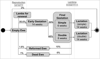
The flock size is a variable that is optimized in the model. Ewes can be made to lamb in three contrasting seasons – spring, autumn or winter – and can produce one or two lambs per reproduction cycle (simple or double), or even three when prolificacy is very high (Benoit, Reference Benoit1998). In this study, we focused on spring lambing season as it corresponds to the natural physiological cycle of ewes. Sheep-for-meat flock management is represented by differentiating categories of animals in function of their evolving physiological needs. For adult ewes, we determined six categories: empty ewes, early-gestation ewes, final simple gestation ewes, final double gestation ewes, simple lactating ewes, and double lactating ewes. The life cycle of a ewe, characterized by changes between these six above mentioned physiological stages, is represented in Figure 2. Dates and percentages of presence of a given ewe category are fixed parameters. Regarding adult males, a constant parameter of one ram for 40 ewes is considered (Benoit, Reference Benoit1998).
State diagram of a ewe (Unified Modeling Language (UML)).

Regarding lambs management, we differentiated four categories: simple males, double males, simple females and double females. For each category, weights after weaning and weights of sales are user-adjustable. It determines the fattening period and the physiological needs of the growing lambs (INRA, 2007). A part of the female lambs may be selected for the renewal of reformed and dead ewes instead of directly purchasing new ewes. In this case, female lambs are led separately to the lamb fattening batch after 30 kg, based on their specific physiological needs (INRA, 2007). Replacement ewes may also be purchased. The number of replacement ewes is determined by mortality, fertility and reform rates.
Feeding constraint
For each category of animals, daily physiological needs were determined using the INRA references (INRA, 2007). Four periods were determined to adjust the equilibrium between physiological needs and feed resources: winter, spring, summer and autumn. Feed resources are on-farm feed production and/or market feed purchases. For instance, in case of mixed crop–livestock production, plant production can be sold as cash crops or stocked on-farm to feed the flock. Specific practices can be run to enhance this availability of on-farm feed, such as intercropping.
The vegetal subsystem
Pasture and crop production
We define pasture production as temporary and permanent grassland. Crop production may correspond to cash crops, fodder crops (i.e maize forage) or crop stored on-farm as feed. Yields are determined by annual parameters for crop production and by seasonal parameters for pasture production. Seasonal parameterization was preferred for pasture production in order to take into account various possible management practices associated to pasture production as hay, silage or pasture. Furthermore, to explicitly consider the effect of rotational patterns on performances, constraints were designed to allow for specific preceding and succeeding vegetal production for each rotational pattern option: crop–crop, pasture-crop or crop–intercrop.
Fertilization constraints
Fertilization needs are determined on an annual basis and depends on the pasture management and on the rotational patterns options. Two resources are available for fertilization: manure and chemical fertilizers. Manure production is calculated proportionally to the duration of presence of ewes and lambs in the sheepfold. The fertilization value of manure is determined by its frequency of spreading and the nature of the vegetal production on which the manure is spread (Supplementary Table S1). If there is not enough manure to compensate fertilization needs, chemical fertilizers are purchased.
Other constraints
Other constraints refer to labor and capital. Regarding labor, its availability is not considered unlimited in the model: a lower and an upper bound are parametrized. The quantity of workers is then a function of the flock size and the total agricultural area. Regarding capital, materials and buildings needed for each farming system simulated are generated in order to evaluate the economic pillar of sustainability, the net income.
Performance indicators
Economic and production performances
The economic performance of farming systems is evaluated by the net income per worker as this indicator permits having a relevant base of comparison. Indeed, the net income is calculated by subtracting the structural charges from the gross margin and by reporting the economic result per worker. Structural charges include the labor costs (social security charges for all the workers), mechanization and building costs (maintenance of equipment and building, and depreciation costs), and land charges (land rent. All the farm land is considered as tenant farming. The tenancy assigned on land property represents the remuneration of farmer’s land asset). Livestock production performance is determined by the quantity of meat produced per hectare mobilized. The concept of ‘hectare mobilized’ reflects the global surface that is needed to conduct the flock. It is composed by the hectares of self-consumed crops, the hectares of pastures and the equivalent hectares of imported feeds. The equivalent hectares are quantified using national reference yields. This concept permits comparing contrasted mixed crop–livestock systems more consistently. Indeed, if only on-farm hectares used for livestock production were considered, the MC–L systems where the flock self-consumes a part of the crop production would obviously be disadvantaged for each indicator expressed on a per-hectare basis. Regarding crop production, results are reported in terms of kilo of plant protein (more relevant than kilo of grain to aggregate cereal grain, oilseed and/or other cash crops) per hectare sold to avoid poor comparisons between farming systems that self-consume crops from those that sell their whole production.
Environmental performances
Farming systems modeled are evaluated through indicators of nitrogen balance, non-renewable energy consumption expressed in mega-joule (MJ) and GHG emissions. Regarding the nitrogen balance, the approach used is the Simon and Le Corre (Reference Simon and Le Corre1992) method for calculating the balance between nitrogen leaving and nitrogen entering the farm (Veysset et al., Reference Veysset, Lherm and Bébin2010). This methodology requires converting each input and output in equivalent nitrogen content (Idele, 1999). Regarding the two last indicators, a life cycle assessment (LCA) method makes it possible to quantify the environmental impacts of a product from raw material extraction up to the moment the product leaves the farm (from the cradle to the farm gate). Here, we used the energy and CO2 coefficients of the LCA Diaterre® method, a reference for energy-GHG audits in France (Ademe, 2010). This methodology permits reporting the environmental impacts by categories of inputs and by type of production – crop or livestock (Veysset et al., Reference Veysset, Lherm and Bébin2010). Regarding livestock production, the categories for MJ consumption are crop self-consumption, feed purchases, fertilizers purchases, other purchases (treatments, seeds, veterinary interventions, etc.), direct energy (fuel, electricity, water), materials and buildings. For GHG emissions, there are two additives categories: methane (CH4) emitted through enteric fermentation and GHG emitted from C-N cycle (nitrogen leaching, manure storage and spreading, dejections, carbon sequestration, etc.). With regards to crop production, the same categories are evaluated apart those that are specific to livestock production.
Parametrization
Livestock subsystem
Flock management is parametrized from a database composed of 40 (mixed crop and) sheep-for-meat farms monitored by our INRA research group since more than 20 years (Farm Economy and Management Team (EGEE), in the Mixed Research Unit on Herbivores (UMRH, INRA)) (Benoit and Laignel, Reference Benoit and Laignel2011). Data from the French Chamber of Agriculture permits calibrating the manure production and the effect of manure management options on its nitrogen value.
Vegetal subsystem
Regarding pasture production, the analysis of representative farms of the Vienne department region permits highlighting three schemes of pasture management (Idele, 2013). The first scheme corresponds to spring silage, summer hay harvest and autumn pasture (Pasture A). The second scheme corresponds to spring pasture, summer hay harvest and autumn pasture (Pasture B). The third scheme corresponds to a full pasture system (Pasture C). These schemes were analyzed using data of Idele (French livestock institute, Idele (2013)) to quantify average hay and silage production and using the experimental SOERE-ACBB database from INRA Lusignan to quantify season-by-season pasture production (SOERE-ACBB). The production consensus reached with experts after comparing this data is reported in Supplementary Table S2. Production values include manipulation and trampling losses. Mineral needs are dependent on pasture management and have been setup based on representatives farms of the Vienne region (Idele, 2013). Note that nitrogen return to soil at pasture is already factored into the mineral needs estimate reported in Supplementary Table S2.
Regarding crop production, we selected two crops rotations schemes representative of lowland areas in France: maize–wheat–barley (MWB), and rapeseed–wheat–barley (RWB). In the case of rotation MWB, we allowed for two kinds of intercrop: white mustard and fodder rapeseed. White mustard is a popular intercrop as it is cheap and easy to manage. Fodder rapeseed is uncommon but recent experimental studies have demonstrated that it carries a number of advantages, mainly its ability to provide good-quality feeds for animals in the September to October period when pasture production is low (Ciirpo, 2008). Crop residues cannot be used as stuble because this practice may lead to animal injuries (legs). Yields and nitrogen needs of each vegetal production are parametrized per rotation scheme to explicitly take into account effects of the preceding crop on the succeeding crop (Supplementary Table S3). This parametrization requested data from SOERE/ACBB experiments (INRA) and other local experimental analysis lead by technical institutions.
Labor, capital and economic context
The relation between the quantity of labor work and the flock size/agricultural area was parametrized using our research-unit database. The parametrization of the capital subsystem was taken from an existing updated model called Ostral (Benoit, Reference Benoit1998). Finally, the model was parametrized on the 2012 economic context and on the 2014 to 2020 Common Agricultural Policy reform context. Given that decoupled aids are set to converge till 2020, the model was parametrized on the expected aids values for 2020, that is a base payment of €92/ha, a green payment of €86/ha and a redistributive payment of €103/ha for each system simulated (France Agricole, 2014).
Simulation
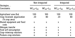
By allowing a controlled environment of simulation, Sheep‘n’Crop allows studying the impact of crop–livestock organization by decomposing its effects in two categories: the direct effects and the indirect effects. The direct effects of crop–livestock organization correspond to changes in management and performances that occur when the percentages of crop and livestock vary. The indirect effects correspond to the impact of crop–livestock organization on the capacity of a MC–L system to enhance its performances through crop–livestock interactions. Concretely, to test the direct effects of crop–livestock organization, two MC–L systems with no crop–livestock interactions other than labor, equipment and fixed costs shared between crop or livestock activities are simulated: one with 20% of the agricultural area dedicated to crop production and the other with 80%. These farming systems are respectively called the non-integrated MC20–L80 system and the non-integrated MC80–L20 system (Table 1). To test the indirect effects, the same two MC–L systems were simulated but this time crop–livestock interactions are allowed as transfer of manure on crops, feed self-consumption and rotational patterns with intercrops or pasture. They are then called the integrated MC20–L80 system and the integrated MC80–L20 system (Table 1). When interactions are allowed, the model can balance the nitrogen and feed requirements with on-farm resources and/or purchased inputs if needed. In all cases, the model optimizes the system in order to maximize the gross margin of the whole farm; it chooses the best economic way, respecting all the constraints, to manage crop and livestock activities (size of the flock, rotation, selling or not crops, when allowed, using all or a part of crop as feed, intensifying or not the production system with a high amount of purchased inputs, etc.). To simulate those systems, we set a labor constraint in order to not exceed two workers per farm (the maximum observed in the region (Idele, 2013)). In the same way, the agricultural area was set at 100 ha according to the mean observed in the region (Idele, 2013). By setting the farm size constant in our simulations, it permits having comparable farm structures to study the direct and indirect effects of crop–livestock organization. There are no capital constraints.
Scenario of simulation to test (i) the direct effect of crop–livestock organization by comparing non-integrated MC20–L80 and MC80–L20 systems and (ii) the indirect effect of crop–livestock organization by comparing the integrated and non-integrated scenarios for both MC20–L80 and MC80–L20 systems

MC20–L80=mixed crop–livestock system with 20% of the agricultural area with crops and 80% of the agricultural area with pastures for livestock; MC80–L20=mixed crop–livestock system with 80% of the agricultural area with crops and 20% of the agricultural area with pastures for livestock; Shared equipment and fixed costs=no crop–livestock interactions other than labor and equipment; x=farming practice allowed; o=farming practice not allowed.
Results
Characterization of the mixed crop–livestock systems
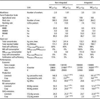
Both non-integrated MC–L systems are running the same crop management, that is rotations with MWB (Table 2). However, regarding livestock management, the stocking rate is of 7.4 livestock units (LU) per hectare for the MC20–L80 system whereas it increases till 13 LU per hectare for the MC80–L20 system. This intensification of the flock management when a higher percentage of crops is run implies a higher consumption of total feed concentrates (241.4 kg per ewe instead of 134.7 for the MC80–L20 system).
Comparison of MC–L systems characteristics according to their crop–livestock organization and integration

MC20–L80=mixed crop–livestock system with 20% of hectares with crops and 80% of hectares with pastures for livestock; MC80–L20=mixed crop–livestock system with 80% of hectares with crops and 80% of hectares with pastures for livestock; MWB=rotation with maize, wheat, barley; MWBR=rotation with maize, wheat, barley, fodder rapeseed as intercrop; PMWB=rotation with six years of pasture and then maize, wheat, barley; P=pastures; ha mob.=hectare mobilized (=total hectares mobilized on- and off-farm to feed the flock); LU=livestock unit; DM=dry matter; FU=feed unit, one FU being equivalent to the average energy produced by 1 kg of barley; WB self-consumption=self-consumption of wheat and barley.
a (X%)=percentage of decrease or increase in performances between MC20–L80 and MC80–L20 systems, for the non-integrated and the integrated scenarios. This percentage is calculated by keeping the highest value as the benchmark.
Regarding integrated MC–L systems, integration practices selected through the optimization problem solving are mainly the same for both MC–L systems: introduction of pasture into the crop rotation, transfer of manure on crops and feed self-consumption (cereal and straw). However, the quantities involved in the interactions are constrained by the contrasted crop–livestock organization of the farming systems studied (Table 2). For instance, 93.3% of the agricultural area is involved into pasture–crop rotations for the MC20–L80 system whereas only 23.3% for the MC80–L20 system. Crop–livestock organization also influences the stocking rate, with 7.4 livestock unit per hectare of pasture for the MC20–L80 system and approximatively 13 for the MC80–L20 system. As a consequence, total concentrates and stocked fodder per ewe are higher for the MC80–L20 system (Table 2). Furthermore, integration leads to a slightly higher stocking rate for the MC80–L20 system whereas no variation is observed for the MC20–L80 system. As a consequence, the feeding management is intensified in the MC80–L20 system (+21.6 kg concentrates/ewe). However, for both systems, the on-farm feeding management scheme permits increasing the feed self-sufficiency up to 98% for the MC80–L20 system and up to 94% for the MC20–L80 system (Table 2). A fodder rapeseed intercrop is conducted in the integrated MC80–L20 system to help reaching this level of feed self-sufficiency. Finally, an increase of fertilization self-sufficiency for both systems is observed and is related to their relative implication in pasture–crop rotation and transfer of manure on crops.
In the following subsections, the impacts of these MC–L characteristics on performances are declined from two points of view: the direct impact of crop–livestock organization on performances – analyzed through the comparison of non-integrated MC–L systems with contrasted crop–livestock organization – and the indirect impact of crop–livestock organization on performances – analyzed through the comparison of the performances gains (or losses) reached by the same two MC–L systems when crop–livestock interactions are adopted.
Direct impact of crop–livestock organization on performances
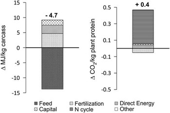
Beyond the effects that crop–livestock organization has on management characteristics, crop–livestock organization has an impact on economic, production and environmental performances of farming systems. Table 2 reports this impact for each indicator of performance by computing the percentage of decrease/increase in performance of both non-integrated MC–L system keeping the highest value as the benchmark. These figures permit highlighting the significant impacts of crop–livestock organization on performances (variation higher than 5%). Those significant impacts are contrasted: a higher percentage of crops has a positive impact on-farm income (+44%), livestock production (+18%) and GHG emissions for crop production (−14%) whereas a negative impact is observed for the nitrogen balance (+53%) and the MJ consumption of livestock production (+9%). Those contrasted effects are mainly explained by two management characteristics, the crop and livestock production scale and the livestock intensification.
Crop and livestock production scale
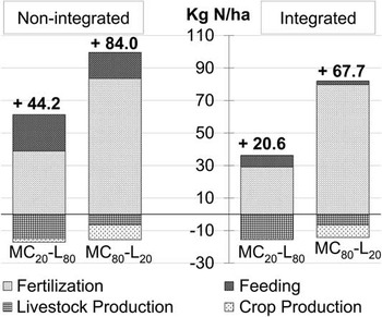
Crop production is more profitable than livestock production. As a consequence, the MC80–L20 system has a net income much higher than the MC20–L80 system even if more aids are granted to the MC20–L80 system given its higher flock size (decoupled aid being equal between systems). In the same way, a higher crop production scale has a positive impact on GHG emissions because the N cycle is less efficient for the MC20–L80 system when no crop–livestock interaction is allowed (Figure 3). However, this management scheme is also responsible for a negative impact on nitrogen balance. Indeed, it is observed on Figure 4 that the exportation of one nitrogen unit through crop production necessitates the importation of much more nitrogen unit for fertilization. Furthermore, a higher flock size permits enhancing fertilization self-sufficiency by reducing the importation of chemical nitrogen on farm. This affects thus again the nitrogen balance in favor of the MC20–L80 system (Figure 4). As a consequence, when the crop production scale increases, the importation of nitrogen increases even more – leading to a much higher nitrogen balance for the MC80–L20 system.
Determinants of the variation in performances (MJ consumption for livestock production and GHG emissions for crop production) of the non-integrated MC20–L80 system in comparison with the non-integrated MC80–L20 system.

Variation in N Balance composition in relation to crop–livestock organization and integration processes.

Livestock intensification
Even if flock size is higher in the MC20–L80 system, the livestock production of the MC80–L20 system is more intensive (+5.6 LU/ha pasture) because less workers are needed per hectare of crop production than for livestock production. More working time is thus available in the MC80–L20 system to increase the stocking rate. As a consequence, performances at the livestock production scale are affected. For instance, the livestock production increases by 18% for the MC80–L20 system. However, the MJ consumption of the MC20–L80 system makes it 9% lower than the MC80–L20 system (Table 2) owing mainly to its lower MJ consumption for feeds (Figure 3). This helps compensate its higher MJ consumption for fertilization relatively to the MC80–L20 system, explained by its less optimal matching between manure resources and fertilization needs at the livestock production scale. Furthermore, as livestock intensification leads to a lower feed self-sufficiency, it directly affects the nitrogen balance of the MC80–L20 system by a much higher nitrogen importation for feed per unit of nitrogen exportation through livestock products (Figure 4). This is the second factor explaining the worse N balance performance for the MC80–L20 system.
Indirect impact of crop–livestock organization: impact of crop–livestock interactions on performances
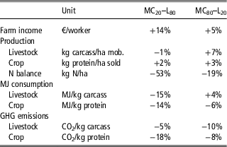
Crop–livestock organization influences the capacity of a MC–L system to enhance economic, production and environmental performances through crop–livestock interactions. Table 3 reports these impacts as the percentage of decrease or increase in performance of an integrated MC–L system when compared to its equivalent non-integrated farming system (i.e. with the same crop–livestock organization). Three categories of results can be highlighted. The first result is that crop–livestock interactions have a positive impact for both MC–L systems (farm income, nitrogen balance, livestock and crop GHG emissions, crop MJ consumption) (Table 3). Second, crop–livestock interactions may influence the performances of only one MC–L system (variation higher than 5%) – depending on its specific crop–livestock organization (livestock production, livestock MJ consumption) (Table 3). Third, a performance – crop production – is not affected by crop–livestock interactions for both MC–L systems (variation lower than 5%) (Table 3). These contrasted results may be explained by changes in farming system management that arise from the adoption of crop–livestock interactions in both MC–L systems: livestock intensification, feed self-sufficiency and nitrogen self-sufficiency.
Impact on performances of crop–livestock interactions adoption in contrasted mixed crop–livestock systems (20% or 80% of crop) – the indirect impact of crop–livestock organization.

Percentage of variation [(integrated−non-integrated)/non-integrated].
MC20–L80=mixed crop–livestock system with 20% of hectares with crops and 80% of hectares with pastures for livestock; MC80–L20=mixed crop–livestock system with 80% of hectares with crops and 80% of hectares with pastures for livestock; ha mob.=hectare mobilized (=total hectares mobilized on- and off-farm to feed the flock).
Livestock intensification
When crop–livestock interactions are conducted, sheep-for-meat production keeps constant for the MC20–L80 system whereas it increases by 7% for the MC80–L20 system. This result is linked to the intensification of the flock observed in the MC80–L20 system when crop and livestock are integrated. This effect is not observed for the mixed crop–livestock system with 80% of crops because the labor constraint yet was saturated, that is the maximum number of two workers to manage the farm yet was reached.
Increasing feed self-sufficiency
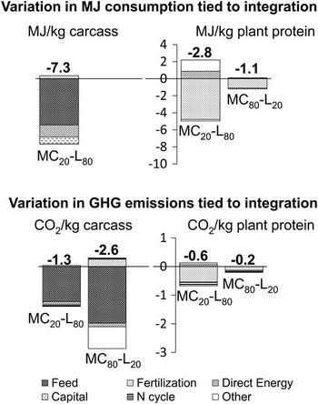
The self-consumption of crops permits enhancing feed self-sufficiency in both systems. This new feed management explains the significant improvements in MJ consumption and GHG emissions for livestock production (Figure 5). This higher feed self-sufficiency is also responsible for the improvement of the nitrogen balance in the MC80–L20 system. Indeed, less nitrogen is imported as feed purchases and it largely compensates the lower quantity of nitrogen exported from crop sales (Figure 4). The variation observed for the crop sales are much lower than that of feed purchased because the total crop self-consumption in N equivalent is very low in comparison with the induced increase in feed self-sufficiency. For instance, regarding the MC80–L20 system, crop self-consumption permits increasing the feed self-sufficiency from 40% to 98% while the total crop self-consumption in N equivalent is of only 16% (i.e. 1.4 kg N/ha) (Table 2).
Determinants of the variation in performances (higher than 5%) observed when crop–livestock interactions are conducted in both MC20–L80 system and MC80–L20 system – The indirect impact of crop–livestock organization.

Increasing nitrogen self-sufficiency
Crop–livestock interactions as rotations with pastures and transfer of manure on crops permit enhancing nitrogen self-sufficiency for both systems (Table 2). The chemical nitrogen fertilization needs are lower for the integrated farming systems because grasslands supply nitrogen in pasture-crop rotations, and the nitrogen value of manure is higher when applied on crops (Supplementary Table S4). The nitrogen self-sufficiency is slightly higher for the MC20–L80 system given its higher manure production and its higher capacity to have pasture–crop rotations (53.3% of the total area – Table 2). As a consequence, the reduction of nitrogen importations tied to fertilization is higher for the MC20–L80 system, which explains why – in this case – it is the nitrogen self-sufficiency that acts as the first factor explaining its nitrogen balance improvement (Figure 4). In the same way, the increase in nitrogen self-sufficiency is correlated to the level of improvements in MJ consumption and GHG emissions for crop production in both MC–L systems (Figure 5).
It has to be noted that the indirect impact of crop–livestock organization don’t reverse the trend imposed by its direct impact. Indeed, the integrated MC80–L20 system keeps the higher performances in terms of farm income, production and GHG emissions for both crop and livestock productions while the integrated MC20–L80 system keeps the best for nitrogen balance and MJ consumption for crop and livestock productions (Table 2). However, when crop–livestock interactions are conducted, the performance gap observed between MC20–L80 and MC80–L20 systems decreases from 44% to 40% for farm income and from −14% to −4% crop GHG emissions. The reverse effect is observed for nitrogen balance (from 47% to 70%), livestock production (from 18% to 24%), livestock MJ consumption (from 9% to 25%), livestock GHG emissions (from −3% to −8%) and crop MJ consumption (from −2% to +7%).
Discussion and perspectives
Trade-off between performances: the direct effect of crop–livestock organization
Our simulations highlight that crop–livestock organization is responsible for trade-off between MC–L systems performances: the best performances are divided between the non-integrated MC20–L80 and MC80–L20 systems. For instance, increasing the percentage of crop production leads to an increasing farm income while at the same time having a negative impact on the N balance. However, as our simulations were conducted in a current economic context that is in favor of crop production and that the economic context influences possibilities for scope and scale economies (Dupraz, Reference Dupraz1998), we tested a contrasted economic conjuncture to discuss our results. In that objective, we run the same farming systems with market prices of 2014, known to be less favorable for crop and more favorable for sheep meat production (Supplementary Table S5). Results show that running a farming system with 80% of crops is again more profitable – even if the economic trade-off is well reduced (Supplementary Table S5).
In the same way, increasing the level of livestock intensification leads to a higher livestock production while at the same time neglecting MJ consumption objectives for livestock production (and N balance). This identification of trade-off between performances associated to the adoption of farming practices is not new. One research stream focused on economic an environmental trade-offs linked to crop–livestock interactions, but without considering crop–livestock organization. For instance, Bell and Moore (Reference Bell and Moore2012) yet had identified through a scientific review that a given practice could not satisfied the whole set of objectives to reach sustainability. In the same way, Parsons et al. (Reference Parsons, Nicholson, Blake, Ketterings, Ramírez-Aviles, Fox, Tedeschi and Cherney2011b) highlighted through a model-based study that the adoption of crop–livestock integration practices led to trade-off between performance objectives. As a last example, Perrot et al. (Reference Perrot, Caillaud and Chambaut2012) showed through a database analysis that a mixed crop–livestock system could have better economic result than a specialized system for livestock production while at the same time having worse environmental performances. Another research stream focused on the trade-offs driven by crop–livestock organization. For instance, Thamo et al. (Reference Thamo, Kingwell and Pannell2013) studied the trade-off between profit and GHG emissions implied by crop–livestock organization, but without considering the impact of crop–livestock interactions. In the same way, other research studies identified that crop–livestock organization as a contrasted impact on profit but without considering environmental performances (Morrison et al., Reference Morrison, Kingwell and Pannell1986; Byrne et al., Reference Byrne, Robertson, Bathgate and Hoque2010). Hence, our result confirms that crop–livestock interactions is not the sole factor leading trade-offs between performances but that crop–livestock organization also drives trade-offs. Our result is new in the sense that it identifies the relative effect of both factors on performances. Indeed, by decomposing the direct and indirect effects of crop–livestock organization, we observed that the effects crop–livestock interactions on performances – even if not equal between systems – could not reverse the trend imposed by crop–livestock organization. As consequence, crop–livestock organization appears to be a key factor that has to be considered when evaluating and comparing sustainability of MC–L systems.
Importance of considering the indirect effect of crop–livestock organization
Our hypothesis that crop–livestock organization has also an indirect effect on performances when crop–livestock interactions are conducted was also confirmed. Indeed, even if crop–livestock interactions don’t reverse the trade-off trend imposed by crop–livestock organization, we observed that the impact of a crop–livestock interaction practice on a given performance is affected by crop–livestock organization. This result suggests again that studies on the capacity of crop–livestock interactions to enhance sustainability of MC–L systems have to be tested on contrasted organizational patterns. Here below, effects of crop–livestock interactions are discussed in depth for each indicator of performance.
Economic performance
Our result suggesting that integrated MC–L systems are in both case more profitable than non-integrated MC–L systems – acting as two juxtaposed specialized system – is opposed to those of Veysset et al. (Reference Veysset, Lherm, Bebin and Roulenc2014) and Ryschawy et al. (Reference Ryschawy, Choisis, Choisis, Joannon and Gibon2012) (France). This contrasted result may be explained by the fact that – in our study – farming systems are compared at the same scale of production preventing bias of evaluation owing to the occurrence of scale economies (Dupraz, Reference Dupraz1998). As we also considered the variation of the fixed costs associated with crop–livestock interactions (buildings, materials), we can state that those interactions have a global positive impact on profitability. One factor explaining that higher profitability is the lower nitrogen needs for fertilization (and thus purchases) when crop–livestock interactions are conducted. Another factor may be the lower price put for on-farm feed consumption than for purchased cereals. This parameterization is in line with the 2012 conjuncture where we observed cereal price volatility. The same simulations run with the 2014 conjuncture – where cereals prices keeps equal – show that integrated systems still keep more profitable (Supplementary Table S5). All those statements have to be confirmed by analyzing other land availability.
Production performances
Regarding livestock production, as the workload constraints the flock size, a slight effect was observed on production because flock size could not increase. Regarding crop production, no significant effect was observed because we considered vegetal protein production and not energy production. Indeed, if we transform the vegetal production into energy equivalent (% starch), the MC20–L80 will benefit more from the crop–livestock interactions (+31% from the baseline without interactions – 4050 kg starch/ha sold) than the MC80–L20 (+6% from the baseline without interactions –4050 kg starch/ha sold). This is explained by the fact that maize has a much higher energy content than other crops and that this production isn’t self-consumed. The gap between crop productions is less pronounced regarding protein contents so that no significant effect is observed.
Environmental performances
Regarding no-renewable energy consumption, our results in favor of integration are consistent with those of Benoit and Laignel (Reference Benoit and Laignel2010) that reported a better energy efficiency for optimized integrated mixed crop–sheep systems (0.93) than for specialized systems (0.42). Regarding GHG emissions and N balance, the positive effect of integration is in line with numerous scientific results (Russelle et al., Reference Russelle, Entz and Franzluebbers2007; Wilkins, Reference Wilkins2008). However, this scientific literature generally concerns evaluation at the biophysical scale – as the coupling of N and C cycles – while our evaluation concerns the farming system scale. At this scale of evaluation, some studies focusing on observed data revealed more contrasted effects of integration on environmental performances. For instance, Veysset et al. (Reference Veysset, Lherm, Bebin and Roulenc2014) reported that specialized suckler beef cattle had better environmental results than mixed crop–livestock systems. In the same way, Ryschawy et al. (Reference Ryschawy, Choisis, Choisis, Joannon and Gibon2012) showed that mixed crop–livestock systems generally reached intermediary levels of performance in comparison with specialized systems. We link these contrasted results to three factors: (i) they compare systems with different scale of production permitting specialized system to exploit higher scale economies, (ii) observed mixed crop–livestock systems do not optimize crop–livestock integration, (ii) observed mixed crop–livestock systems face to agronomical and technical constraints (as workload) that prevent obtaining results reported by simulation models or by studies conducted at the biophysical level.
Model limits and perspectives
We especially recommend improving the consideration of the social pillar of sustainability. Indeed, our model takes into account the impact crop–livestock organization on workload but not that of crop–livestock interactions. Furthermore, the necessity to develop some more technical and organizational skills for managing MC–L systems is not considered. To address this, some authors proposed to develop an indicator of viability of farming systems (Chauvat and Servière, Reference Chauvat and Servière2005; Cournut and Chauvat, Reference Cournut and Chauvat2010). However, quantifying this indicator needs to have sufficient data to distinguish seasonal and on-call worker at a daily scale (Dedieu et al., Reference Dedieu, Coulomb, Servière and Tchakerian2000; Madelrieux et al., Reference Madelrieux, Dedieu, Dobremez and Girard2009). On-call work concerns work that cannot be postponed, like lambing, whereas seasonal work concerns tasks that can be postponed, as fences maintenance. Further detailed on-farm data are thus needed to cope with that pillar of sustainability.
We also suggest improving the genericity of our model regarding the impact of vegetal rotations on yields and nitrogen needs. Indeed, we parametrized the model with experimental data and decisions of fertilization do not seem rationale given that a worst N balance performance is observed when more crops are run. As a consequence, even if our results represent a reality, the genericity of our model could be improved by integrating a more accurate management of fertilization and associated yields in function of vegetal rotations.
Conclusions
Mixed crop–livestock systems are claimed more sustainable than specialized systems. However, conditions of integration that permits MC–L systems being more sustainable than specialized systems are not well understood. We developed the concept of crop–livestock organization, translating the allocation of the total agricultural area between crop and pasture production. We showed that crop–livestock organization, a factor usually not considered when comparing MC–L systems and specialized systems, is a main factor explaining performances of MC–L systems. Indeed, even if crop–livestock interactions improve global performances as mentioned in the scientific literature, crop–livestock organization is responsible for the existence of trade-off between objectives of sustainability. As a consequence, without the design of policies allowing for higher economic incentives to mix crop and livestock productions, the crop specialization will progress in the Vienne department till the total disappearing of sheep-for-meat production – that is an undesirable situation regarding environmental indicators (and production self-sufficiency).
This result first implies that both crop–livestock organization and crop–livestock interactions have to be considered when discussing and comparing performances of MC–L and specialized farming systems. Second, this result corroborates the need for further trade-off analysis to understand which MC–L system to sustain, that is which MC–L system corresponds to the best compromise between objectives of sustainability.
Acknowledgments
The authors are grateful for financial support from the French National Institute for Agricultural Research (INRA-Phase/SAE2) and the French Environment and Energy Management Agency (Ademe). Many thanks to Gabriel Laignel and both reviewers for their helpful comments.
Supplementary material
To view supplementary material for this article, please visit http://dx.doi.org/10.1017/S1751731116000720