

Introduction
At least two levels of organisation of communities are usually distinguished in parasitology: the infracommunity, that is, the totality of parasites inhabiting a single host individual, and the component community, that is, the totality of parasites identified in the local host population (Bush et al. Reference Bush, Lafferty, Lotz and Shostak1997; Holmes and Price Reference Holmes, Price, Kikkawa and Anderson1986; Poulin Reference Poulin1997). The structuring of communities at these levels is influenced by a continuum of conditions, including the individual characteristics of the host, the history of formation of the local parasite fauna, and the abiotic and biotic factors affecting the abundance, spatial distribution, and other parameters of the populations of the intermediate and the definitive hosts (e.g., Holmes Reference Holmes, Esch, Bush and Aho1990; Timi and Lanfranchi Reference Timi and Lanfranchi2009).
The decay of community similarity with increasing geographic distance is one of the most widely discussed macroecological patterns of parasite communities (e.g., Poulin and Morand Reference Poulin and Morand1999; Poulin Reference Poulin2003; Fellis and Esch Reference Fellis and Esch2005; Seifertová et al. Reference Seifertová, Vyskočilova, Morand and Šimkova2008; Pérez-del-Olmo et al. Reference Pérez-del-Olmo, Fernández, Raga, Kostadinova and Morand2009; Locke et al. Reference Locke, Levy, Marcogliese, Ackerman and McLaughlin2012; Chai et al. Reference Chai, Bennett and Poulin2022). This effect is not always pronounced (Bezerra et al. Reference Bezerra, Pinheiro, de Melo, Zanchi-Silva, Queiroz, dos Anjos, Harris and Borges-Nojosa2016; Locke et al. Reference Locke, Levy, Marcogliese, Ackerman and McLaughlin2012; Warburton et al. Reference Warburton, Kohler and Vonhof2016), with the degree of its manifestation strongly depending on the level of parasite community organisation. For instance, the similarity decay of infracommunities with geographic distance is generally more pronounced than that of component communities (Pérez-del-Olmo et al. Reference Pérez-del-Olmo, Fernández, Raga, Kostadinova and Morand2009; Timi et al. Reference Timi, Lanfranchi and Luque2010). Furthermore, in the case of highly vagile hosts such as migratory birds, an important factor affecting the manifestation of the distance decay in the similarity of the parasite communities is the spatial scale of the study (Locke et al. Reference Locke, Levy, Marcogliese, Ackerman and McLaughlin2012).
Aquatic birds are traditionally regarded as hosts colonised by a particularly species-rich parasite fauna (Bush et al. Reference Bush, Aho and Kennedy1990). This is due to their trophic strategy, which is based on a wide range of invertebrate and vertebrate organisms, as well as their close association with aquatic ecosystems, where most of the intermediate hosts of trematodes and cestodes are concentrated. The significant role of trophic specialisation and ecological plasticity of aquatic birds in the structuring of both infracommunities and component communities of their parasites has been repeatedly demonstrated in parasitological studies (e.g., Buscher Reference Buscher1965; Alexander and McLaughlin Reference Alexander and McLaughlin1997; Labriola and Suriano Reference Labriola and Suriano2001; Navarro et al. Reference Navarro, Lluch and Font2005; Skirnisson Reference Skirnisson2015; Stapf-Skiba and Kavetska Reference Stapf-Skiba and Kavetska2019; Lorenti et al. Reference Lorenti, Cremonte, Minardi, Bertellotti, Navone and Diaz2025).
Eurasian Coot Fulica atra Linnaeus, 1758 is a particularly promising model object for ecological studies of parasite communities in this context. This species has a broad geographical distribution and a high abundance in many regions; it also shows considerable plasticity in respect of habitat choice, nesting both in large lakes and reservoirs and in small isolated water bodies (Kurochkin Reference Kurochkin, Potapov and Flint1987). The high vagility of the coot potentially facilitates the transfer of its parasites along migration routes and their exchange between different territorial groups of the host (Fedynich and Pence Reference Fedynich and Pence1994). At the same time, the life cycles of most of these parasites are rigidly limited by the conditions in the specific water bodies, which determine the presence of appropriate intermediate hosts as well as the share of the animal component in the diet in different coot individuals. The diet of coots mainly consists of aquatic plants but usually includes some animal prey (Metna et al. Reference Metna, Lardjane-Hamiti, Boukhemza-Zemmouri, Boukhemza, Merabet and Abba2015; Sakai Reference Sakai2015). The parasite fauna of the coot has been extensively studied (e.g., Creplin Reference Creplin1829; Diesing Reference Diesing1861; Pukhov Reference Pukhov1939; Ginetsinskaya Reference Ginetzinskaja1952; Macko Reference Macko1956; Sey Reference Sey1966; Pavlov Reference Pavlov1962; Babička and Vojtek Reference Babička and Vojtek1972; Pojmańska Reference Pojmańska1982; Kulišić et al. Reference Kulišić, Lepojev, Aleksić-Bakrač, Jakić, Pavlović, Milutinović and Mišić2004; Birmani Reference Birmani2011; Yakovleva et al. Reference Yakovleva, Lebedeva and Bugmyrin2021), with some recent studies employing the methods of integrative taxonomy (Vlasenkov et al. Reference Vlasenkov, Kalmykov and Sokolov2023, Reference Vlasenkov, Akimova and Sokolov2024a, Reference Vlasenkov, Shchelkanov and Sokolov2024b, Reference Vlasenkov, Gordeev and Sokolov2025a, Reference Vlasenkov, Lipkovich and Sokolov2025b, Reference Vlasenkov, Shchelkanov and Sokolov2025c, Reference Vlasenkov, Shchelkanov and Sokolov2025d, Reference Vlasenkov, Yakovleva and Sokolov2025e). However, the spatial variability of the parasite communities of the coot remains unclear.
The aim of this study was to analyse the structure of parasite communities of the Eurasian Coot using comparative and biogeographic approaches. Particular attention was paid to the role of distance in structuring the spatial variability of these communities.
Material and methods
Host examination and parasite collection
Coots were shot by licensed hunters near seven water bodies located in different regions of Eurasia within the boundaries of Russia and Belarus (Table 1; Figure 1). Samples from each locality were represented by 15 specimens of Eurasian Coots and included adult males, adult females, and juveniles. Parasitological dissection followed the standard protocol (Dubinina Reference Dubinina1955, Reference Dubinina1971). We collected only helminths, ignoring other parasitic organisms such as protists, insects, etc.
Collection localities

Table 1. Long description
The table contains seven columns: Locality (region), Water body, Females, Males, Adults/Juveniles, Coordinates, and Date of sampling.
* Rostov (Rostov Region, Russia): River Mokraya Chuburka; 9 females, 6 males; 4/11 adults/juveniles; 46.74565679954144 degrees North, 39.15378028818987 degrees East; September 2023.
* Belarus (Minsk Region, Belarus): Lake Naroch; 10 females, 5 males; 6/9 adults/juveniles; 54.89596343520356 degrees North, 26.731153025873553 degrees East; September 2023.
* Khasan (Primorsky Krai, Russia): Lake Maloe Krugloe; 7 females, 8 males; 12/3 adults/juveniles; 42.38469184619868 degrees North, 130.71605920520722 degrees East; October 2023.
* Kaliningrad (Kaliningrad Region, Russia): Lake Valetniki; 8 females, 7 males; 3/12 adults/juveniles; 54.54784954353677 degrees North, 20.024533314413922 degrees East; September 2024.
* Khanka (Primorsky Krai, Russia): Lake Khanka; 8 females, 7 males; 3/12 adults/juveniles; 44.72347154002758 degrees North, 132.06991462364508 degrees East; September 2024.
* Tver (Tver Region, Russia): Ivankovo Reservoir; 8 females, 7 males; 7/8 adults/juveniles; 56.56103386337917 degrees North, 36.23607439979044 degrees East; August 2025.
* Orsk (Orenburg Region, Russia): Lake Shalkar-Ega-Kara; 9 females, 6 males; 8/7 adults/juveniles; 50.78736718161429 degrees North, 60.91084617749059 degrees East; September 2025.
Map showing sampling locations of Eurasian coots examined for parasites in Eurasia. (A) General map. (B) Sampling localities in Belarus, European and Ural Regions of Russia. (C) Sampling localities in the Russian Far East. Abbreviations of locations: 1, Kaliningrad (Lake Valetniki); 2, Belarus (Lake Naroch); 3, Tver (Ivankovo Reservoir); 4, Rostov (River Mokraya Chuburka); 5, Orsk (Lake Shalkar-Ega-Kara); 6, Khanka (Lake Khanka); 7, Khasan (Lake Maloe Krugloe). Scale bars: A = 500 km; B = 200 km; C = 100 km.

Figure 1. Long description
Panel A is a large map of Eurasia with two blue rectangular insets labeled B and C. Inset B is on the Western side and Inset C is on the Eastern side. A scale bar representing 500 km is at the bottom left.
Panel B, located at the bottom left, is a detailed view of the Western region with a 200 km scale bar. It contains five red dots numbered 1 through 5.
* Point 1 is the furthest West at Kaliningrad.
* Point 2 is East of point 1 in Belarus.
* Point 3 is Northeast of point 2 in Tver.
* Point 4 is South of point 3 near Rostov.
* Point 5 is the furthest East in this panel at Orsk.
Panel C, located at the bottom right, is a detailed view of the Russian Far East with a 100 km scale bar. It contains two red dots.
* Point 6 is located North at Khanka.
* Point 7 is located South of point 6 at Khasan.
The helminth species were identified based on molecular and/or morphological characters. Taxonomic information and phylogenetic data on many helminth species parasitising Eurasian Coots from the above localities have been published in our previous studies (Vlasenkov et al. Reference Vlasenkov, Akimova and Sokolov2024a, Reference Vlasenkov, Shchelkanov and Sokolov2024b, Reference Vlasenkov, Gordeev and Sokolov2025a, Reference Vlasenkov, Lipkovich and Sokolov2025b, Reference Vlasenkov, Shchelkanov and Sokolov2025c, Reference Vlasenkov, Shchelkanov and Sokolov2025d, Reference Vlasenkov, Yakovleva and Sokolov2025e). Identification of other helminth species was performed according to Khokhlova (Reference Khokhlova1986), Tolkacheva (Reference Tolkacheva1991), Lomakin (Reference Lomakin1991, Reference Lomakin1993), Niewiadomska (Reference Niewiadomska2010, Reference Niewiadomska2015), Dronen and Blend (Reference Dronen and Blend2015), Heneberg et al. (Reference Heneberg, Sitko and Bizos2015), Niewiadomska and Pojmanska (Reference Niewiadomska and Pojmańska2018), and Sokolov et al. (Reference Sokolov, Kalmykov, Frolov and Atopkin2022). In the current study, we obtained a partial sequence of the mitochondrial cytochrome c oxidase subunit 1 gene for one specimen of the acanthocephalan Filicollis anatis (Schrank, 1788) collected from the Kaliningrad Region of Russia. DNA was extracted according to Holterman et al. (Reference Holterman, van der Wurff, van den Elsen, van Megen, Bongers, Holovachov, Bakker and Helder2006). Polymerase chain reaction (PCR) was performed in a total volume of 25 μL using the Encyclo Plus PCR kit (Evrogene, Moscow, Russia) according to the manufacturer’s instructions and a BIO-RAD T100 Thermal Cycler. The sequence was amplified using the primers and PCR cycling conditions described by Bowles et al. (Reference Bowles, Blair and McManus1992). The PCR product was purified using the PCR Cleanup S-Cap extraction kit (Evrogene, Company, Moscow, Russia) and sequenced for both DNA strands at the ‘Genome’ Shared Resource Centre (Engelhardt Institute of Molecular Biology RAS, Moscow, Russia). Sequencing data obtained in this study have been deposited in the GenBank database of the National Center for Biotechnology Information (NCBI) under the accession number PZ769265 (443 bp).
Parasitological indices were calculated in accordance with Bush et al. (Reference Bush, Lafferty, Lotz and Shostak1997).
Statistical analysis
The data were processed in MS Excel and R 4.0.1 (R Core Team, 2026) environments using basic functions (stats) and functions from packages ‘vegan’ (Oksanen et al. Reference Oksanen, Simpson, Blanchet, Kindt, Legendre and Minchin2025), ‘jakR’ (Kimbrel Reference Kimbrel2024), ‘psych’ (Revelle Reference Revelle2026), and ‘mvnormtest’ (Jarek Reference Jarek2024).
Differences between parasite infracommunities were studied using permutation multivariate analysis of variance (PERMANOVA, vegan::adonis2) with the number of replicates B = 999. The Euclidean distance was used as a metric in two modifications: for binary data (presence or absence of the species in the infracommunity) and for quantitative data (ln-transformed number of specimens of the species in the infracommunity). The significance of age and sex differences between infracommunities from each locality was assessed using a two-way PERMANOVA, while differences between the sets of infracommunities from different localities (below simplified to ‘between localities’) were assessed using a one-way PERMANOVA. The key statistic, pseudo-F, is the ratio of intragroup to intergroup variance (equivalent to the Fisher F-value in ANOVA). The difference between the groups (proportion of variance explained, ‘strength of effect’) is estimated by coefficient R² on a scale from 0 to 1, while the significance level p is determined by Monte Carlo Randomisation (MCR-test). Post hoc tests with Holm’s correction for the significance level p were used for pairwise comparisons of these groups (jakR::pairwiseAdonis). The uniformity of intragroup variances, including post hoc pairwise comparisons, was assessed using the test for multivariate homogeneity of variances (PERMDISP) after calculating the principal coordinates of infracommunities (metric multidimensional scaling, PCoA) in two-dimensional space (vegan::betadisper). The absence of significant differences between the variances supported the conclusion obtained with the use of PERMANOVA about the significance of centroid differences between the localities.
The main variability trends of prevalence and mean abundance of parasite species in the component communities were established by principal component analysis (PCA). To reduce the observed variability, the values of mean abundance were ln-transformed before the analysis. Variances and factor loadings were calculated using the correlation matrices of the traits (stats::princomp with argument cor = TRUE, stats::loadings). Bartlett’s χ 2 sphericity test (psych::cortest.bartlett) indicated that both correlation matrices were significantly different from the identity matrices (Bartlett’s χ 2 > 182.55, df = 21, p < 0.001) and were suitable for PCA. The significant trends were identified by principal components with an eigenvalue of at least one. The share of the principal component in the total variance is a measure of its information value, in other words, an indicator of the strength of the effect. Variability trends were established based on the identified clusters of factor loadings and the ‘+’ or ‘–’ sign, indicating a direct or inverse relationship between the traits. Only the traits with a relative load of at least 0.7 (relative to the largest absolute load value for a given component) were included in the clusters. The contribution of the remaining traits was considered insignificant.
The association between the observed dissimilarity of the component communities and the geographic distances between the corresponding localities was established using correlation analysis. Non-linear effects were minimised by transforming the original distances between the localities and the dissimilarity metrics between the communities into principal coordinate values by metric multidimensional scaling (PCoA) with the use of Q-technique of PCA. Principal coordinates, which are equivalent to factor loadings in PCA, were calculated from the double-centred symmetric matrices of distances between all the objects (Davis Reference Davis1986; stats::cmdscale; S1 in Supplementary materials). Geographic distances were represented by (1) the matrix of ln-transformed values of the shortest distances between points of material collection (103 km), (2) the matrix of longitudinal distances (parallels, °E), and (3) the matrix of latitudinal distances (meridians, °N). The component communities of the parasites were compared pairwise using the Euclidean metric, and principal coordinates were then calculated from the obtained matrices of (i) species composition, (ii) prevalence, and (iii) ln-transformed mean abundance. Finally, all calculated PCoA axes were scaled from −1 to +1 according to the formula: each absolute value of principal coordinate/square root of eigenvalue of the same axis. The relative values of the principal coordinates of the localities and the communities in the samples compiled for the correlation analysis did not formally differ from a two-dimensional normal distribution (mvnormtest::mshapiro.test, Shapiro–Wilk W < 0.921, p > 0.309). Nevertheless, because of the small size of the samples, we chose Spearman’s non-parametric method (stats::cor.test with the argument ‘spearman’). The significance of differences between correlation coefficients from zero was established using Monte Carlo Randomisation (MCR-test) with a number of iterations B = 999. Correlations between geographic distance matrices and community dissimilarity matrices were compared using the Mantel permutation method (vegan::mantel with the argument ‘spearman’).
Whenever we tested several samples and found significant differences in the text after ‘>’ and ‘<’ signs, we gave the lowest value of the statistic and the highest significance level of the p-value, respectively, out of all calculated values. Conversely, when the differences in the text after ‘>’ and ‘<’ signs were non-significant, we gave the highest value of the statistic and the lowest significance level of the p-value, respectively.
Results
Altogether, we examined 105 coots from seven localities in the Palaearctic. Uninfected coots were present only in samples from Rostov (one bird) and Khasan (two birds). In total, 6041 parasite specimens were found in the remaining birds. The parasites belonged to 24 taxa, which, for the purpose of this study, were considered as units of species richness (Table 2). These taxa were represented by 19 nominal species, two taxa at the genus rank that were not differentiated into nominal species either because of the technical difficulties in accurately estimating the infection indices for each species (Diorchis spp.) or because of the presence of numerous subadult specimens that could not be identified to the species level (Notocotylus spp.), two taxa at the genus and family levels that were not identified because of poor preservation of the material (Cotylurus sp., Capillariidae gen. sp.), and one taxon of the genus level that probably represents a new species awaiting nomenclatural proposals (Hyptiasmus sp. of Vlasenkov et al. [Reference Vlasenkov, Yakovleva and Sokolov2025e]). All parasite specimens, except for immature Notocotylus sp. (Table 2), were gravid.
Species composition of parasites from Eurasian Coot in the studied localities and infection indices: P – prevalence, %, I – infection intensity, ind., A – mean abundance, ind.

Table 2. Long description
The table details parasite species across Kaliningrad, Belarus, Tver, Rostov, Orsk, Khasan, and Khanka.
* Platyhelminthes, Trematoda: Includes 19 species. Notable entries include Cyclocoelum mutabile (cyc) with prevalence ranging from 6.7 percent in Belarus to 66.7 percent in Orsk. Notocotylus species (not) show high prevalence in Tver at 93.3 percent and Belarus/Rostov at 73.3 percent. Neomoliniella bancrofti fulicae (neo) is most prevalent in Rostov at 60.0 percent.
* Platyhelminthes, Cestoda: Diorchis species (dio) show 100 percent prevalence in Kaliningrad, Belarus, Tver, and Orsk, with the highest mean abundance in Tver at 113.40.
* Acanthocephala, Palaeacanthocephala: Filicollis anatis (fil) is present in Kaliningrad (26.7 percent), Belarus (6.7 percent), and Tver (6.7 percent).
* Nematoda, Enoplea: Capillariidae species (cap) appear in Kaliningrad, Belarus, and Khasan with low prevalence (6.7 to 13.3 percent).
* Nematoda, Chromadorea: Quasiamidostomum fulicae (qus) is widespread, peaking at 73.3 percent prevalence in Rostov. Pelecitus fulicaeatrae (pel) is found in Kaliningrad, Tver, Khasan, and Khanka.
Indices used are P for prevalence in percent, I for infection intensity range, and A for mean abundance.
Note: aAbbreviated names are used as species labels in Figure 3; bCo-occurrence of gravid Notocotylus pacifera, Notocotylus sp. of Vlasenkov et al (2025) and immature specimens of Notocotylus sp. in different combinations; cCo-occurrence of several Diorchis spp. in different combinations: Diorchis acuminata (Clerc, 1902), Diorchis americana Ransom, 1909, Diorchis brevis sensu lato 1 Rybicka, 1957, Diorchis brevis sensu lato 2, Diorchis cf. longibursa Steelman, 1939, Diorchis inflata (Rudolphi, 1819).
The infracommunities comprised 1–9 taxa. The parasite infracommunities at each of the seven sites showed no statistically significant differences in species composition or abundance that could be attributed to the age or sex of the hosts (two-way PERMANOVA pseudo-F < 1.238, df = 3, 11, R2 < 0.252, p > 0.250). The dispersions within these groups were homogeneous in all localities (PERMDISP F < 4.199, df = 1, 13, p > 0.059). Therefore, we did not divide the host samples based on age and sex. The polygons grouping the infracommunities from each locality based on their species composition and abundance overlapped considerably (Figure 2). Nevertheless, in both cases, the centroids formed two relatively well-distinguished geographic groups, represented by the more compact northern group (Kaliningrad–Belarus–Tver) and the less compact southern group (Rostov–Khasan–Khanka). Orsk locality occupied an intermediate position between these groups due to its unstable position in the principal coordinate axes calculated from dissimilarity matrices in composition and abundance of the species.
Ordination of parasite infracommunities of Eurasian Coot in principal coordinate axes (PCo) based on their species composition (A) and the number of parasite specimens (B). The crosses and circles mark infracommunities and centroids of localities, respectively.

Figure 2. Long description
A two-panel attribute space diagram.
Panel A: Ordination based on species composition. The horizontal axis is P Co 1 ranging from negative 1.8 to 1.2. The vertical axis is P Co 2 ranging from negative 1.0 to 1.5. Seven overlapping convex hulls in various colors (red, blue, purple, yellow, green, orange, and grey) contain circular data points representing infracommunities. A black cross inside a colored square marks the centroid for each locality. The clusters are highly concentrated and overlapping in the center of the plot between P Co 1 values of negative 0.8 and 0.7.
Panel B: Ordination based on the number of parasite specimens. The horizontal axis is P Co 1 ranging from negative 6.0 to 6.0. The vertical axis is P Co 2 ranging from negative 8.0 to 4.0. The clusters show greater separation compared to Panel A. The red cluster (Orsk) is shifted toward the bottom-left (negative P Co 1 and negative P Co 2), while the grey (Khasan) and purple (Rostov) clusters are shifted toward the right (positive P Co 1).
A legend at the bottom identifies the seven localities: Kaliningrad (yellow), Belarus (orange), Tver (green), Rostov (purple), Orsk (red), Khanka (blue), and Khasan (grey). Each legend entry shows a square with a cross and a solid circle in the corresponding color.
The differences between localities were statistically significant both in respect of the composition of the parasite infracommunities and the abundance of the species in them (one-way PERMANOVA pseudo-F < 3.905, df = 6, 98, R2 < 0.300, p < 0.001), but with an overall inequality of variances (PERMDISP pseudo-F < 4.825, df = 6, 98, p < 0.002). Pairwise comparisons of the variances indicated the existence of two homogeneous clusters of localities (PERMDISP p > 0.079), their members differing significantly from each other in intergroup pairs (PERMDISP p < 0.041). In terms of species composition, these clusters were Kaliningrad–Rostov–Khanka and Belarus–Tver–Orsk–Khasan, the infracommunities in the former being more variable than in the latter. In terms of species abundance, clusters of a slightly different composition emerged, namely, Kaliningrad–Rostov–Orsk–Khanka and Belarus–Tver–Khasan, the infracommunities being more variable in the former. Homogeneity of variances verified the differences in the centroids of localities revealed by PERMANOVA within each cluster, while the intergroup differences were not obvious, as they could also be explained by the dispersion of infracommunities. Pairwise differences between the centroids were pronounced in various degrees (Table 3). For instance, intergroup differences in the species composition were quite obvious in the pairs of localities Khasan–Tver, Khasan–Orsk, and Rostov–Belarus, while intergroup differences in the abundance were more pronounced in the pairs of localities Khasan–Tver, Khasan–Belarus, Khasan–Orsk, and Rostov–Tver. Nevertheless, the differences between geographically more distant localities could be only slightly more pronounced or even less pronounced than the differences between geographically closer ones. For instance, this was the case in the Kaliningrad–Tver–Khanka series in the analysis of the species composition and in the Kaliningrad–Khanka–Khasan series in the analysis of parasite species abundance.
Values of statistic R2 obtained after pairwise comparison of the centroids for geographic groups of the parasite infracommunities (PERMANOVA, results of post hoc tests)

Table 3. Long description
The table compares seven localities: Kaliningrad, Belarus, Tver, Rostov, Orsk, Khasan, and Khanka. The main diagonal consists of double equals signs where a locality is compared to itself.
Values above the diagonal represent differentiation based on species composition:
* Kaliningrad vs: Belarus 0.072, Tver 0.042, Rostov 0.140, Orsk 0.091, Khasan 0.155, Khanka 0.089.
* Belarus vs: Tver 0.076, Rostov 0.174, Orsk 0.166, Khasan 0.172, Khanka 0.151.
* Tver vs: Rostov 0.139, Orsk 0.094, Khasan 0.213, Khanka 0.100.
* Rostov vs: Orsk 0.097, Khasan 0.117, Khanka 0.097.
* Orsk vs: Khasan 0.197, Khanka 0.055 (bolded).
* Khasan vs: Khanka 0.109.
Values below the diagonal represent differentiation based on mean ln-transformed abundance:
* Belarus vs Kaliningrad: 0.097.
* Tver vs: Kaliningrad 0.130, Belarus 0.076.
* Rostov vs: Kaliningrad 0.216, Belarus 0.288, Tver 0.306.
* Orsk vs: Kaliningrad 0.115, Belarus 0.191, Tver 0.145, Rostov 0.218.
* Khasan vs: Kaliningrad 0.208, Belarus 0.317, Tver 0.387, Rostov 0.149, Orsk 0.309.
* Khanka vs: Kaliningrad 0.114, Belarus 0.227, Tver 0.227, Rostov 0.126, Orsk 0.150, Khasan 0.114.
All differences are statistically significant with p less than 0.021, except for the bolded value of 0.055 between Orsk and Khanka which has a p value of 0.151.
Note: Estimates of differentiation based on species composition are given above the diagonal; estimates based on mean ln-transformed abundance of species are given below the diagonal; all differences between localities are statistically significant (p < 0.021) except the value given in bold (p = 0.151).
The component communities comprised 8–16 taxa (Table 2). The Mantel test did not reveal any significant positive relationship between the dissimilarity matrices of component communities in terms of species composition, prevalence, and mean abundance of species and the matrices of geographic distances (Spearman correlation coefficient rs < −0.001, p < 0.456).
The PCA based on species composition identified three patterns of variability in the component communities of the Eurasian Coot (three significant principal components, Table 4). These components accounted for approximately 75% of the total variance of the primary data. Along the first component, the parasite species were ranked based on their prevalence within the communities: core species such as the trematodes Notocotylus spp., Cyclocoelum mutabile (Zeder, 1800), Neomoliniella bancrofti fulicae Macko, 1968 and Tanaisia atra (Nezlobinsky, 1926), the cestodes Diorchis spp. and the nematode Quasiamidostomum fulicae (Rudolphi, 1819) had the highest values, whilst satellite species had values below zero (Figure 3A). The component communities from Orsk, Khasan, Khanka and Tver, which were the most similar in terms of the composition of the core species, had peak factor loadings. The parasite community from Rostov gravitated towards this group, having the highest relative value of factor loading for PC-1, but was less similar to it in respect of species composition in general. The second component captured the specificity of the component community from Kaliningrad locality, which was mainly associated with the presence of species that had the maximum values for this component: the trematodes Cyathocotyle bithyniae Sudarikov, 1974 and Metorchis xanthosomus (Creplin, 1846), the nematode Capillariidae gen. sp. and the acanthocephala Filicollis anatis (Schrank, 1788). Judging by the factor loadings, the same parasite species determined the similarity between the component communities from Kaliningrad and Belarus as well as the dissimilarity between these two communities on the one hand and the community from Khanka locality on the other hand. The specificity of the component community from Belarus locality by the third component was due to the trematode Apopharynx bolodes (Braun, 1902) as well as the trematodes Dendritobilharzia pulverulenta (Braun, 1901) and Echinostoma cf. sarcinum Dietz, 1909 (Figure 3B). The presence of the latter two species explains the relatively high similarity between Belarus and Rostov.
Variability of the parasite species composition in the component communities, their prevalence and mean abundance along the axes of the significant principal components (PC, the results of principal component analysis)

Table 4. Long description
The table is organized into eight columns. The first column lists Localities and their abbreviated names. The subsequent columns are grouped under three main categories: Species composition (P C 1, P C 2, P C 3), Prevalence P (P C 1, P C 2), and Mean abundance ln A (P C 1, P C 2).
Data rows by locality:
* Kaliningrad Kl: Species composition (0.151, 0.721, -0.274); Prevalence (0.381, -0.399); Mean abundance (0.309, -0.611).
* Belarus Bl: Species composition (0.125, 0.441, 0.759); Prevalence (0.372, -0.470); Mean abundance (0.291, -0.558).
* Tver Tv: Species composition (0.400, 0.130, -0.408); Prevalence (0.397, -0.306); Mean abundance (0.409, blank).
* Rostov Rs: Species composition (0.347, -0.319, 0.365); Prevalence (0.347, 0.555); Mean abundance (0.353, 0.448).
* Orsk Or: Species composition (0.532, -0.053, 0.150); Prevalence (0.423, 0.130); Mean abundance (0.443, 0.180).
* Khasan Ks: Species composition (0.447, 0.188, -0.069); Prevalence (0.341, 0.423); Mean abundance (0.404, blank).
* Khanka Kn: Species composition (0.446, -0.360, -0.147); Prevalence (0.378, 0.150); Mean abundance (0.411, 0.270).
Statistical summary rows:
* Eigenvalues: Species composition (2.88, 1.34, 1.03); Prevalence (2.22, 0.86); Mean abundance (2.09, 0.98).
* Percentage of total variance: Species composition (41.20, 19.16, 14.68); Prevalence (73.41, 11.00); Mean abundance (64.89, 14.19).
Note: Factor loadings with relative weights greater than 0.7 are highlighted in bold in the original table. Bartlett’s sphericity test results: chi-squared greater than 35.09, d f equals 21, p less than 0.027.
Note: Factor loadings with relative weights greater than 0.7 are highlighted in bold. Gaps indicate factor loadings with values close to zero. All correlation matrices are suitable for PCA (Bartlett’s sphericity test: χ 2 > 35.09, df = 21, p < 0.027). Abbreviated names were used as locality labels in Figures 3 and 4.
Ordination of parasite species in principal component (PC) axes based on composition of component communities from the studied localities (A and B), and their prevalence (C) and mean abundance (D) in these communities. The arrows indicate factor loadings (see Table 4); the actual values for the labels on the edges of the diagram were limited to −2 or 2.

Figure 3. Long description
A multi-panel figure containing four scatter plots labeled A, B, C, and D. Each plot features a central origin at 0,0 with red factor loading arrows pointing toward specific localities.
Panel A: P C-1 on the x-axis and P C-2 on the y-axis, both ranging from minus 2.0 to 2.0. Red arrows radiate from the center toward the right, labeled Kaliningrad, Belarus, Khasan, Tver, hoc, Orsk, Khanka, and Rostov. Gray square data points representing species like cap, fil, and cbt are scattered primarily in the top-left and right-hand margins.
Panel B: P C-2 on the x-axis and P C-3 on the y-axis. Red arrows point toward Belarus (top-right), Rostov and Orsk (top-left), Khanka (middle-left), and Tver, Kaliningrad, and Khasan (bottom-right). Species points like esr and apo are in the upper quadrants, while psi and ct2 are in the lower-left.
Panel C: P C-1 on the x-axis and P C-2 on the y-axis. Red arrows are concentrated on the right side, pointing toward Rostov, Khasan, Khanka, Orsk, Tver, Kaliningrad, and Belarus. A dense cluster of species points including cfl, psi, pel, and cap is located in the middle-left quadrant.
Panel D: P C-1 on the x-axis and P C-2 on the y-axis. Red arrows point toward Rostov, Khanka, Orsk, Khasan, Tver, Belarus, and Kaliningrad on the right. Species points are more widely dispersed on the left, with neo at the top-right and dio at the bottom-right edge.
The results of PCA of the parasite prevalence indicate two main directions of variability of the component communities (Table 4). The first principal component, explaining 73% of the total variance, can be defined as the structure of the group of core species. In this case, the factor loadings formed a general trend with an emphasis on the component community of parasites from Orsk. The species that were recorded within the infracommunities more frequently than the others had the highest values of this component (Figure 3C). In the order of decreasing values, these were Diorchis spp., Notocotylus spp., Q. fulicae, C. mutabile “and” T. atra. They can be regarded as the core species of the parasite communities of the coot in northern Eurasia. The remaining species occurred sporadically within the communities and could be classified as satellite species. However, some of them, such as C. bithyniae, Hyptiasmus oculeus Kossack, 1911, N. b. fulicae, and Prosthogonimus ovatus (Rudolphi, 1803), made a significant contribution to the communities in certain localities and can be identified as local core species. The variance of the second component was below the significance level, which was taken as 1, and its contribution to the total variance was small, only 11%. Nevertheless, this component was important because it managed to reveal the geographic differentiation, identifying two directions of variability of the component communities. The more northerly localities, especially Kaliningrad and Belarus, were opposed to the more southerly ones, Rostov and Khasan. The former localities were characterised by a high prevalence of Diorchis spp. and C. bithyniae, while the characteristic features of the latter were a high prevalence of N. b. fulicae and Q. fulicae (Figure 3C). In addition, the more northern component communities contained two parasites that were not recorded in the southern localities (Rostov and Khanka): F. anatis and M. xanthosomus.
Similar results were obtained in the analysis of the mean abundance of the parasites (Figure 3D). The first two principal components, explaining 65% and 14% of the total variation, respectively, identified the same trends. The group of core species remained unchanged; however, in the southern group of localities mentioned above, T. atra replaced Q. fulicae at the top of the list. The geographic differentiation of the localities based on the presence of satellite species became more pronounced. For instance, the specificity of southern localities, particularly those in the Black Sea basin (Rostov), was more pronounced due to the presence of the trematode Cyathocotyle fulicae Ginetzinskaja, Reference Ginetzinskaja1952 and the higher abundance of the trematode D. pulverulenta as compared to the other localities.
Thus, the PCA revealed several trends of geographic variability in the data. For a detailed interpretation of these results, each pattern of variation has to be separated from the influence of the others as much as possible. One way of achieving this is to determine the principal coordinates of the traits using the Q-technique of PCA within the framework of metric scaling in Euclidean space (PCoA). The calculation of the principal coordinates based on the matrix of the shortest geographic distances between the localities yielded two axes (PCo 1 and PCo 2), the share of the total variance being 97% and 3%, respectively (S2 in Supplementary materials). The distribution of the values of the principal coordinates of the localities along the first axis was found to be closely correlated with their longitudinal position (Spearman’s correlation coefficient: rs = 0.929, p = 0.003). The second axis showed no significant linear relationships with either longitude or latitude (rs < 0.357, p > 0.385); in residual variance, it appears to have captured the regional specificity of the relative positions of the localities. After subtracting the longitude component from the original matrix, the north-western localities (Kaliningrad and Belarus), which were close to each other, had the lowest principal coordinate values, while Rostov and Orsk, which, firstly, were remote from the other localities and, secondly, were the only localities examined in their regions (Azov region and Ural region, respectively), had the highest values.
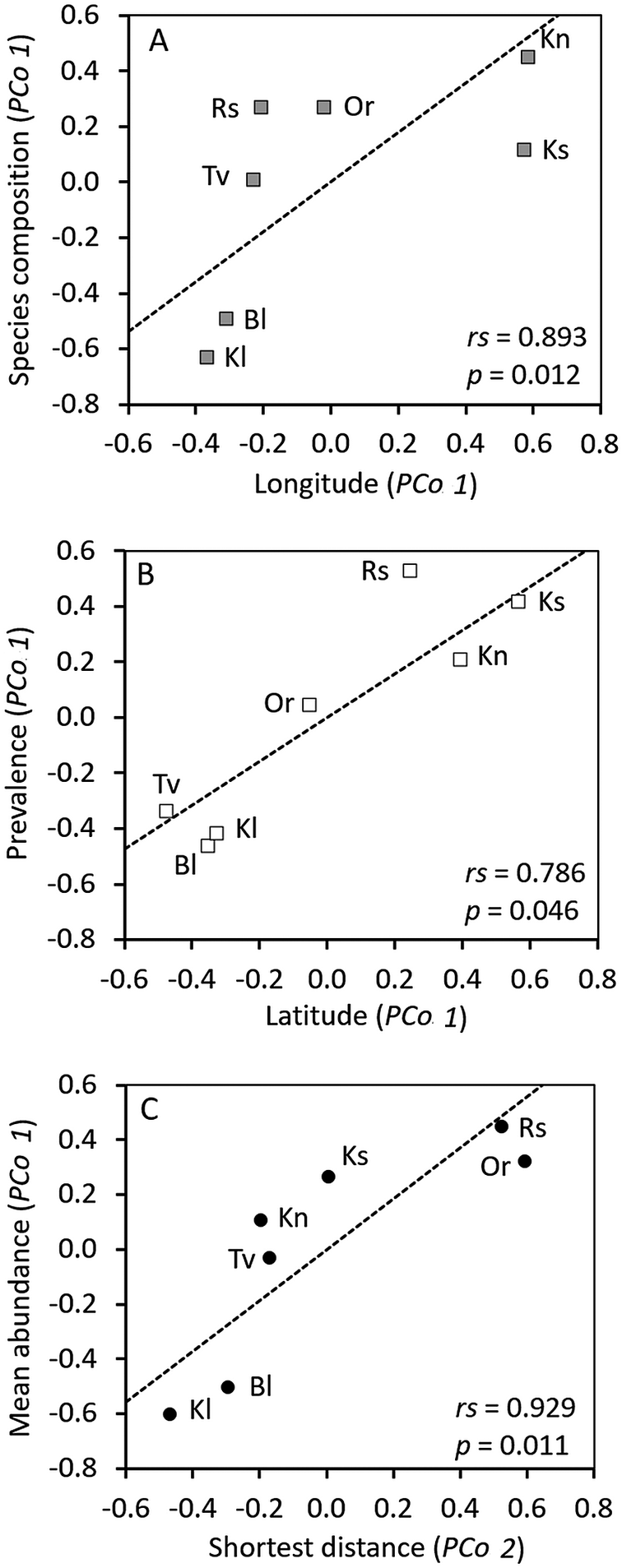
The scaling of the component communities according to species composition, prevalence, and mean abundance of the parasite species yielded four significant principal coordinate axes in each case. Together, they accounted for up to 90% of the initial variability, with the first axis accounting for 32–39%, the second axis, for 20–27%, the third axis, for 16–17%, and the fourth axis, for 9–12%. The results of the study of correlations between the principal coordinate values of the component communities along each of the PCoA axes and the corresponding localities, scaled by the geographic distances between them, indicated a significant correlation only in the following three pairs: species composition (along the first axis, Figure 4A) – longitude, prevalence (along the first axis, Figure 4B) – latitude, mean abundance (along the first axis, Figure 4C) – shortest geographic distance (along the second axis). As expected, the shortest geographic distance along the first axis showed a relatively strong correlation with the species composition (Spearman’s correlation coefficient: rs = 0.714, p = 0.082), since the position of localities along this axis correlated strongly with their principal coordinates along the longitudinal axis (see above). In essence, the correlation of the first pair of traits was repeated here, but in this case the correlation was insignificant.
Similarity decay of the parasite communities with increasing distance between the localities. The lines indicate trend lines with Spearman’s correlation coefficients rs as measures of proportionality; p-values indicate the significance of their differences from zero (MCR-test).

Figure 4. Long description
A multi-panel figure containing three scatter plots labeled A, B, and C. All plots share a Y-axis range from negative 0.8 to 0.6 and an X-axis range from negative 0.6 to 0.8. Each plot features a dashed diagonal trend line and several labeled data points.
* Panel A: The Y-axis is Species composition (P C o 1) and the X-axis is Longitude (P C o 1). Data points include K l and B l in the bottom-left quadrant, T v, R s, and O r in the top-left quadrant, and K s and K n in the top-right quadrant. Statistical values are r s equals 0.893 and p equals 0.012.
* Panel B: The Y-axis is Prevalence (P C o 1) and the X-axis is Latitude (P C o 1). Data points B l, K l, and T v are in the bottom-left quadrant. O r is near the origin. R s, K n, and K s are in the top-right quadrant. Statistical values are r s equals 0.786 and p equals 0.046.
* Panel C: The Y-axis is Mean abundance (P C o 1) and the X-axis is Shortest distance (P C o 2). Data points K l and B l are in the bottom-left quadrant. T v, K n, K s, O r, and R s form a linear progression into the top-right quadrant. Statistical values are r s equals 0.929 and p equals 0.011.
Thus, the differences in the species composition of the parasite component communities of the Eurasian coot increased consistently with increasing longitudinal distance between the localities, while the differences in the prevalence increased with increasing latitudinal distance. The differentiation of the component communities by the mean abundance was mostly determined by the specificity of local conditions.
Discussion
Altogether, 180 helminth species have been recorded in Eurasian Coot from the Palaearctic (Akramova et al. Reference Akramova, Shakarbaev, Arepbaev, Yorkulov, Saidova, Saparov, Mirzaeva, Hamrokulova, Turemuratova, Turemuratova and Azimov2024; Birmani Reference Birmani2011; Dorzhiev et al. Reference Dorzhiev, Badmaeva and Dugarov2021; Gvozdev et al. Reference Gvozdev, Maksimova, Akhmetova, Belyakova, Dobrokhotova, Kukashev, Kulkina and Gvozdev1985; Kondratova et al. Reference Kondratova, Ivanyushina and Penkina2019; Ku Reference Ku1938; Mahmudova Reference Mahmudova2012, Reference Mahmudova2013; Mahmudova and Ibrahimov Reference Mahmudova and ShR2020; Malysheva Reference Malysheva2023; Meggitt Reference Meggitt1927; Mhaisen Reference Mhaisen1994; Mirozova et al. Reference Mirozova, Feyzulaeva, Dadasheva and Mikailov1990; Nicoll Reference Nicoll1923; Olteanu et al. Reference Olteanu, Lungu and Popescu1968; Ricci and Carrescia Reference Ricci and Carrescia1961; Vainutis et al. Reference Vainutis, Voronova, Andreev and Shchelkanov2023; Vlasenkov et al. Reference Vlasenkov, Gordeev and Sokolov2025a, Reference Vlasenkov, Lipkovich and Sokolov2025b, Reference Vlasenkov, Yakovleva and Sokolov2025e; Yakovleva et al. Reference Yakovleva, Lebedeva and Bugmyrin2021; Zhang et al. Reference Zhang, Bu, Huang, Wen and Zhang2012; Table 2). In this study we examined the material from seven localities and found only 16.7% of the Palaearctic helminth fauna of the coot (taking into account the actual species composition of Diorchis spp. and Notocotylus spp.; see Table 2). It should be noted that some of the approximately 150 helminth species recorded in the Eurasian Coot within the Palaearctic but not found in our study have been detected at the boundary between the Palaearctic and the Indo-Malayan zoogeographic realms (Birmani Reference Birmani2011), and so their presence in the areas we surveyed appears unlikely. Some other of these 150 species, while occurring in more northerly regions of the Palaearctic, have been recorded extremely rarely. For example, trematodes of the family Philophthalmidae have been reported in the Eurasian Coot in the Palaearctic only three times in the entire 200-year history of helminthological studies of this bird (Mirozova et al. Reference Mirozova, Feyzulaeva, Dadasheva and Mikailov1990). Finally, we consider the identification of some helminth species found in the Eurasian Coot in the Palaearctic by our predecessors to be questionable. For example, Echinostoma danubiana Olteanu, Lungu & Popescu, Reference Olteanu, Lungu and Popescu1968 and Neomoliniella longicorpa Vainutis, Voronova, Andreev & Shchelkanov, Reference Vainutis, Voronova, Andreev and Shchelkanov2023 are probably conspecific with N. b. fulicae (Vlasenkov et al. Reference Vlasenkov, Shchelkanov and Sokolov2025c). This means that the differences between the number of helminth species identified in our study and in the literature can be largely attributed to objective reasons (different study areas, rarity of parasite species) and probable taxonomic errors made by previous authors.
All the helminths found in our study are specific parasites of rallid birds (Rallidae) or are shared by rallids and anatids (Bykhovskaya-Pavlovskaya Reference Bykhovskaya-Pavlovskaya1962). With the exception of D. pulverulenta, all these helminths infect the coot via the alimentary route: the birds get infected upon ingestion of the free-living larvae or larvae encysted on aquatic plants or molluscan shells (e.g., Q. fulicae, Psilotrema oligoon (von Linstow, 1887), Notocotylus spp.), or the larvae developing within the body of an intermediate host, namely copepods (Diorchis spp.), mallophages (Pelecitus fulicaeatrae (Diesing, Reference Diesing1861)), aquatic isopods (F. anatis), odonates (P. ovatus), fish (M. xanthosomus) and aquatic gastropods (many other trematodes) (Anderson Reference Anderson2000; Khokhlova Reference Khokhlova1986; Niewiadomska Reference Niewiadomska2010, Reference Niewiadomska2015; Niewiadomska and Pojmanska Reference Niewiadomska and Pojmańska2018; Odening Reference Odening1966; Tolkacheva Reference Tolkacheva1991).
Our studies in Belarus, the European part of Russia, and the Orenburg Region were conducted from late August to the middle of September, that is, just before the start of the mass autumn migration of Eurasian Coot (Blum Reference Blum1973; Koshelev Reference Koshelev1984; Noskov et al. Reference Noskov, Rymkevich and Gaginskaya2016). During this period, the coots congregate in the large water bodies, moving there from the nearby breeding habitats (Koshelev, Reference Koshelev1984). This circumstance as well as clear parasitological differences between the samples from different localities (Table 2) indicates that we studied local coots (that is, coots associated with the locality during the current breeding season) rather than a mixture of migrants from different regions. Far Eastern samples of the coots were collected in the second half of September – the first half of October and may have included, in addition to local birds, migrants from further afar. However, we consider this probability to be fairly low, as Eurasian coots are rare in the Far East outside the Primorsky Krai. It should be noted that the samples of the coot from different localities were collected in different years (2023–2025) because of the limitations related to the processing time of the collected material, large distances between locations, the length of the hunting season, etc. However, our analysis with the use of PERMANOVA indicates that the parasite communities studied in the same year are no more similar to each other than to those studied in different years. The PCA also does not reveal any abnormally strong relationships between the communities studied in the same year compared to those studied in different years. Based on these two arguments, we consider the time factor unimportant for the purposes of this study.
As mentioned above, distance decay in similarity of parasite communities is expressed in varying degrees in different host groups, depending on the level of communities (infra- or component communities), or may not be expressed at all (e.g., Pérez-del-Olmo et al. Reference Pérez-del-Olmo, Fernández, Raga, Kostadinova and Morand2009; Timi et al. Reference Timi, Lanfranchi and Luque2010; Locke et al. Reference Locke, Levy, Marcogliese, Ackerman and McLaughlin2012; Warburton et al. Reference Warburton, Kohler and Vonhof2016; Bezerra et al. Reference Bezerra, Pinheiro, de Melo, Zanchi-Silva, Queiroz, dos Anjos, Harris and Borges-Nojosa2016). The presence of multidirectional variability in the data series may be one of the reasons why spatial differences in parasite communities remain unproven, the usual approach being to look for an association between this variability and a single axis of geographic distance using, e.g., the Mantel test. In our opinion, the analysis of spatial patterns of parasite communities should include (i) a reconnaissance study exploring the directions of variability of the communities (using, e.g., PCA), and (ii) a careful disentanglement of the relationships provisionally identified in the reconnaissance study. Where there are two or more significant trends, particular care should be taken to separate each trend from the influence of the others. This can be achieved by metric scaling in Euclidean space (PCoA, see Methods).
Intragroup differentiation of the parasite infracommunities in the localities examined in our study was statistically significantly smaller than the intergroup differentiation (between the localities) in terms of both species composition and mean abundance. However, intergroup differences in species composition could not be properly visualised graphically (Figure 2A) due to the high variability of the infracommunities by this trait. The low prevalence of most of the locally common parasites against the background of a relatively high prevalence of the few broadly widespread species as well as that of the relatively widespread species which had a highly variable (i.e., the least stable in the spatial range) prevalence makes their combinations largely random. As a result, infracommunities from the same locality appear as distant, while infracommunities from distant localities are grouped together in unpredictable ways. Widespread species with a relatively high prevalence are Diorchis spp., Q. fulicae, and Notocotylus spp. The other helminth species determine the regional specificity of the infracommunities. For instance, C. fulicae was found only in Rostov, whereas H. oculeus, found in four other localities, was absent in Rostov (Table 2). However, it should be noted that Witenberg (Reference Witenberg1923) recorded H. oculeus (as Transcoelum sigillum Witenberg, Reference Witenberg1923) in coots near Rostov more than a hundred years ago.
The analysis of the infracommunities in terms of parasite abundance (Figure 2B) revealed a more pronounced latitudinal geographic trend. It may be associated with the changes in the temperature regime of the water bodies from north to south. The temperature regime affects the species composition and the biomass of aquatic macrophytes and invertebrates (intermediate hosts of parasites), which are, respectively, the main and the secondary (or accidental) food items of coots in summer (Koshelev Reference Koshelev1984; Metna et al. Reference Metna, Lardjane-Hamiti, Boukhemza-Zemmouri, Boukhemza, Merabet and Abba2015; Okrut and Stepanenko Reference Okrut and Stepanenko2014; Sakai Reference Sakai2015). The hypothesis that the patterns of parasite communities are associated with the latitude-dependent features of the temperature regime of the water bodies is based on the assumption that the infection of the coots in our study was local (see above).
The component communities of the parasites were differentiated more clearly. The ordination of species in the principal component axes (Figure 3) indicates the relative contribution of each species to this differentiation. Two to three significant directions of variability of the communities were identified in terms of parasite species composition (Figure 3A–B), the prevalence (Figure 3C), and the mean abundance (Figure 3D). Elucidation of the geographic trends identified by PCA with the use of metric scaling (PCoA) made it possible to explain about 40% of the total variability in terms of these indicators. All the dependencies, identified and potentially possible, were associated with the first principal component axes of these traits, while the following axes did not reveal any significant relationships with geographic distances. Their variability could have been due to other reasons, probably to the random combinations of the variants.
Geographic differences in parasite species composition – both at the level of local faunas and at the level of communities of different hierarchical ranks – are a well-known biogeographic feature, which, however, does not exhibit any universal patterns (Johnson and Haas Reference Johnson and Haas2021; Poulin Reference Poulin2010; Rohde and Heap Reference Rohde and Heap1998; Timi et al. Reference Timi, Lanfranchi and Luque2010). We identified the trend of similarity decay in the species composition of the component communities of Eurasian Coot associated with increasing longitudinal distance between the localities (Figure 4A). It is known that coots breeding in Belarus and Kaliningrad Region migrate mainly in western and south-western directions, spending the winter in different regions of Western and Central Europe and North Africa (Blum and Litsbarsky Reference Blum, Litsbarsky, Mikhelson and Viksne1982; Fetisov Reference Fetisov2005; Kharitonov et al. Reference Kharitonov, Kharitonova, Konyukhov, Panov and Litvin2024; Noskov et al. Reference Noskov, Rymkevich and Gaginskaya2016). The main migration corridors of the coots from Tver Region (Tver locality) are not fully understood. Preliminary data on the seasonal migration of these birds from the central part of European Russia, to which Tver Region belongs, indicate movements in both westerly and southwesterly directions, with the latter probably bypassing Belarus and Kaliningrad Region (Kharitonov et al. Reference Kharitonov, Kharitonova, Konyukhov, Panov and Litvin2024). According to Kuznetsova et al. (Reference Kuznetsova, Blokhin, Grevtsev and Zheleznovа2025), coots breeding in the Rostov region of Russia (Rostov locality) either show resident behaviour, making minor seasonal migrations along the coast of the Azov Sea, or migrate in southern and south-western directions to Southern Europe and West Asia. The map of seasonal migrations of coots published by Kharitonov et al. (Reference Kharitonov, Kharitonova, Konyukhov, Panov and Litvin2024) indicates that there is an additional migration corridor linking Belarus and western parts of European Russia (Belarus and Kaliningrad localities) with the Rostov Region of Russia (Rostov locality). However, the intensity of migration along this corridor is low. The coots breeding in the Orenburg Region of Russia (Orsk locality) migrate southwards and overwinter in India, the north-eastern part of West Asia and the southern part of Central Asia (Koshelev Reference Koshelev1984; Kharitonov et al. Reference Kharitonov, Kharitonova, Konyukhov, Panov and Litvin2024). The coots breeding in the Far East migrate to central and southern parts of Japan, to South Korea and to the lower reaches of the River Yangtze (Brazil Reference Brazil2009; Glushchenko et al. Reference Glushchenko, Korobov, Korobova, Vyalkov, Tiunov, Khodakov and Pryadun2022; Kurochkin and Koshelev Reference Kurochkin, Koshelev, Potapov and Flint1987; Moores and Kim Reference Moores and Kim2014; The Ornithological Society of Japan 2012) and Southeast Asia (Blum and Litsbarsky Reference Blum, Litsbarsky, Mikhelson and Viksne1982; Glushchenko et al. Reference Glushchenko, Korobov, Korobova, Vyalkov, Tiunov, Khodakov and Pryadun2022; Kharitonov et al. Reference Kharitonov, Kharitonova, Konyukhov, Panov and Litvin2024). This means that coots from Kaliningrad and Belarus localities share a common migration corridor, which does not overlap (or overlaps weakly) with those of coots from Tver (presumably), Rostov, Orsk, Khanka and Khasan localities. At the same time, the migration corridors of coots from Tver, Rostov and Orsk do not intersect with each other and with those of birds from the two Far Eastern localities; the latter, however, have a common migration corridor. Thus, migration corridors coincide completely in coots from localities closest to each other in respect of longitudinal distance (Kaliningrad and Belarus; Khanka and Khasan) and diverge completely in coots from localities separated by the greatest longitudinal distance (Orsk and all other localities; Khanka–Khasan and all other localities) (Figure 1; Table 1; S2 in Supplementary materials). Unfortunately, the migration routes of other Palaearctic rallid species that serve as hosts for the same helminths as the Eurasian Coot have been studied very little (Kharitonov et al. Reference Kharitonov, Kharitonova, Konyukhov, Panov and Litvin2024). We assume that the longitudinal trend of similarity decay of species composition of the component communities of coots is largely determined by the directions of their seasonal migrations, which promote or prevent the exchange of parasite species between geographically isolated areas. Thus, our results support the opinion that migration corridors are one of the key factors in structuring the diversity of parasites of migratory birds (Fedynich and Pence Reference Fedynich and Pence1994; Wallace and Pence Reference Wallace and Pence1986).
The trend of similarity decay of the component communities in terms of prevalence, which is associated with the increasing latitudinal distance between the localities, is probably a manifestation of the same pattern that we identified based on the scaling of intra-communities, namely, the clustering of localities into the southern group (Rostov, Khanka and Khasan) and the northern group (Tver, Kaliningrad, Belarus), with the group represented by Orsk occupying an intermediate position. Similarly to the case of infracommunities, the trend observed for the component communities is probably associated with the latitudinal gradient of the temperature regime of the water bodies, which affects the species composition and/or biomass of the main (aquatic macrophytes) and the secondary (invertebrates, including intermediate hosts of the parasites) food items of coots.
The mean abundance of parasites was the most variable trait. This can be explained both by the natural range of fluctuations in the population and by the random selection of the host individuals for the study. Studies of fluctuations in the abundance of different animal groups show that population dynamics may be synchronous or asynchronous both at the landscape and at the intercontinental level and that they may depend both on external factors, including global changes, and on intrapopulation processes, including dispersal of individuals (Bjørnstad et al. Reference Bjørnstad, Ims and Lambin1999; Blasius et al. Reference Blasius, Huppert and Stone1999; Hood et al. Reference Hood, Dey and Zelmer2024; Liebhold et al. Reference Liebhold, Walter, Koenig and Bjørnstad2004; Zelmer and Seed Reference Zelmer and Seed2004). Possible combinations of species distribution in respect of abundance associated with annual fluctuations of the size of their local populations appear to be even more geographically unpredictable. Therefore, in general, we consider the association between the mean abundance and the shortest geographic distances between the localities shown in our study as unstable, reflecting local and seasonal specificity of our material. The similarity of the component communities in terms of mean abundance observed in the case of Kaliningrad and Belarus and in case of Khasan and Khanka (Figure 4C) can be easily explained by their geographical proximity and the common migration routes used by the coots from these localities. It is also unsurprising that the component communities in Rostov and Orsk were quite distinct from those in other localities (Figure 4C). Rostov and Orsk are remote from two Far Eastern (Khanka, Khasan) and three more northerly East European localities (Belarus, Kaliningrad, Tver), and, moreover, are the only localities examined in their regions (Azov region and Ural region, respectively). However, the structure of the component communities from the north-western localities, especially Tver, shows a greater similarity to the Far Eastern localities, even though they are separated by the greatest geographic distance.
Overall, the shortest geographic distances turned out to be a less informative measure of differences between the parasite communities than the longitudinal and latitudinal distances. Even the first principal coordinate axis of the localities, which is interpreted as the shortest geographical distances between them, did not reveal any statistically significant association with the differences between communities in species composition.
Supplementary material
The supplementary material for this article can be found at http://doi.org/10.1017/S0022149X2610220X.
Acknowledgements
The authors are grateful to Drs. L.N. Akimova, A.V. Davygora, A.D. Lipkovich, V.I. Nikolaev, O.A. Novozhilov and M.Yu. Shchelkanov for their assistance in collecting the material.
Financial support
The study was funded by the Russian Academy of Sciences, project no. FFER-2024-0027 (Sokolov SG, Vlasenkov SA).
Competing interests
The authors declare that they have no known competing financial interests or personal relationships that could have influenced the work reported in this paper.
Ethical standard
The authors assert that all procedures contributing to this work comply with the ethical standards of the relevant national and institutional guidelines on the care and use of laboratory animals.