1. Introduction
Figure 1 shows the two sides of an object in the collection of the Toitū Otago Settlers Museum in Dunedin, New Zealand. It is 6 inches long and made of ivory. It was originally owned by Captain Andrew Jamieson Elles, master of the Philip Laing, which on 15 April, 1848 became the second immigrant ship to arrive in Dunedin.
Front and back view of an ivory Plane Scale originally owned by Captain Andrew Jamieson Elles. Collection of Toitū Otago Settlers Museum, Dunedin; 1926/37/2.

The object is a Plane (or Plain) Scale used for navigation to solve problems in plane and spherical trigonometry.
The Plane Scale in some form dates back at least as far back as the early 17th century (Waters, Reference Waters1958, p. 446). Bion (Reference Bion1723) describes their construction and use noting that
‘… Plain Scales are commonly of these two Lengths, viz. some one foot long, and others, which are put into Cases of Instruments, but half a foot in Length; and on one Side is a Diagonal Scale: they are generally made of box, and sometimes of Brass or Ivory.’
Most of the scales on the Plane Scale were adopted by Gunter rules and are known collectively as goniometric scales. Gunter rules were larger, and also incorporated logarithmic scales for performing calculations (van Poelje, Reference van Poelje2004a).
The purpose of this paper is to describe the scales found on the Plane Scale and how they were used with particular attention to the secant, tangent and semi-tangent scales. After stereographic projection of the surface of the sphere onto the plane, these scales were designed to streamline geometric constructions used in the graphical solution of navigational problems on the sphere. The methods are fast and efficient, but seem to be very little known today.
2. The scales
Plane Scales are intended to be used with dividers that transfer lengths between scales or to and from a drawing or plot. The scales themselves are made by taking measurements of a geometrical construction based on a reference circle of radius R, as shown in Figure 2. A simplified version is shown in Figure 3. For the Plane Scale in Figure 1, R = 2 inches.
Geometric construction for the Plane Scale (Bion, Reference Bion1723). Figure restored by Rougeux (Reference Rougeux2022).

Simplified diagram of the lengths used in the construction of the scales of the Plane Scale.

2.1. Front side scales
2.1.1. L E (Leagues)
This uniform linear scale can represent leagues or other convenient measure that the user might wish to assign to it when solving problems graphically. The fact that there are 3 divisions per inch suggests that it was intended to represent nautical miles as there are 3 nautical miles in a league. Linear scales are normally identifiable by the presence of a ‘forerunner’ of finer divisions at their beginning. With the dividers set to a length taken from a plot, one end is placed on a major scale division, 10, 20, 30 etc., so that the other end falls on the forerunner from which the second digit of the measurement can be read.
2.1.2. R U (Rhumbs)
The length of the chord CH is shown in Figure 3. The angle, θ, is given in terms of marine compass points. Traditionally, the full circle was divided into 32 compass points differing by 360°/32 = 11¼°. The 8 points on this scale correspond to 90°. The location of markings on the scale is given by x = 2 R sin(5 ⅝° p) for p in compass points.
2.1.3. P
Another linear scale identified as such by its forerunner. Eight divisions on this scale correspond to the reference circle radius R. This is somewhat unusual as there are more commonly ten divisions.
2.1.4. C H (Chord)
The length of the chord CH is shown in Figure 3 with the angle, θ, given in degrees. The chord of 60° is equal to the radius, R, of the reference circle which is frequently needed in plots. Instructions will therefore often tell the reader to ‘Take in your Compasses 60 Degrees from the Line of Chords, and describe the Arc…’ (Bion, Reference Bion1723, p. 34) or similar. The scales RU and CH are most often used when plotting or measuring angles using dividers and hence function as a protractor. The locations of markings on the scale are given by x = 2 R sin(θ/2) for θ in degrees.
2.1.5. M LON (Nautical Miles in a degree of Longitude)
A nautical mile subtends one minute of arc on the Earth’s surface. One degree of longitude measured along the equator is therefore 60 nautical miles in length. Moving away from the equator, the lines of longitude or meridians converge and eventually all meet at the poles. Therefore, the number of nautical miles in one degree of longitude, M, decreases as latitude, θ, increases and is given by M = 60 cos θ.
This scale is used in conjunction with the CH scale. Set one end of the dividers on zero on the CH scale and the other on the required latitude. Transfer this setting to the M LON scale by placing one end of the dividers on 60 and the read nautical miles from the other. For example, at latitude 60°, there are 30 nautical miles in a degree of longitude measured along that parallel of latitude.
The locations of markings on the scale measured from 60 on the left-hand end are given by
 $x = R\sqrt {2 - M/30} $
.
2.1.6. S I (Sine)
The length of the line segment SH is shown in Figure 3. The locations of markings on the scale measured from zero at its left-hand end are
 $x = R\sin \theta $
for angle θ.
2.1.7. SEC (Secant)
The length 0T is shown in Figure 3. This scale is positioned to the right of 90° on the S I scale and represents the secant function, sec θ ≡ 1/cos θ. Measured from zero on the left-hand end of the S I scale, the locations of markings on the SEC scale are given by
 $x = R\sec \theta $
.
2.1.8. T A (Tangent)
The length CT is shown in Figure 3. The locations of markings on the scale measured from zero at its left-hand end are
 $x = R\tan \theta $
for angle θ.
2.1.9. S ·T (Semi-tangent)
The length 0P is shown in Figure 3. Along with the secant (SEC) and tangent (TA) scales, this scale is used in the graphical solution to problems in spherical trigonometry by stereographic projection. The location of markings on the scale measured from zero at its left-hand end are x = R tan (θ/2) for angle θ.
2.2. Back side scales
In the upper part, there are two scales both 6 inches in length running from right to left. The first has major divisions of 1 inch subdivided into tenths. Below it is a scale with major divisions 1.2 inches in length labelled 10, 20,…, 50 and also subdivided into tenths. These scales are similar to those found on Gunter rules which Mackay (Reference Mackay1802, p. 2) describes as follows.
I. A line of inches, each of which is ſubdivided into ten equal parts.
II. A scale of equal parts, in which the foot is divided into ten equal parts, and each of theſe principal diviſions is again ſubdivided into ten equal parts. Theſe two are uſeful in conſtructing figures.
Taken together, the two scales can be used to convert between inches and decimal fractions of a foot with the labels on the lower scale being interpreted as 1.0, 2.0,…, 5.0.
On the lower part of the Plane Scale is a rectangular grid with vertical lines spaced at quarter-inch intervals. At the top, running from right to left are markings at half-inch intervals labelled from 1 to 9. Labels at the bottom run from 1 to 18 from left to right at quarter-inch intervals.
The slanted lines at either end of the rectangular grid are known as diagonals (van Poelje, Reference van Poelje2004b). Taken as a whole, this grid allows lengths spanned by dividers to be set or read to 3-significant-figure accuracy.
Diagonals, like forerunners mentioned previously in connection with the linear scales, LE and P, are placed at the start of the scale with which they are to be used. Hence, the finer grid on the left is associated with the quarter-inch scale at the bottom and those on the right is associated with the half-inch scale at the top.
To read a measurement taken with dividers, one tip is placed on a division in the rectangular grid such that the other tip falls somewhere in the associated grid of diagonals. The first digit is read from the position of the tip in the rectangular grid. The dividers are moved vertically up or down until the other tip falls on a point where horizontal and diagonal lines cross. The second and third digits are then read from the numbers to the side and top (if present) of the diagonal grid, respectively.
3. Some historical background
One of the earliest comprehensive descriptions of a Plane Scale was given by Aspley (Reference Aspley1624) in his Speculum Nauticum. He includes an illustration of one side that shows just three scales corresponding to LE, RU and CH on the device in Figure 1. There are also two scales on the back that Aspley (Reference Aspley1624, p. 10) calls the first and second Lines of Longitude. These are not illustrated but from their general description and by working through examples given in the text explaining how they should be used, it can be deduced that the first is the analogue of the M LON scale in units of leagues and nautical miles with 3 miles to the league. The second Line of Longitude is a 2-cycle logarithmic scale.
In the three books contained within his work The Mariner’s Plain Scale New Plain’d, Collins (Reference Collins1659) describes how the Plane Scale could be used to solve problems in navigation and in plane and spherical trigonometry. Like many works of this type, it is essentially a recipe book with little or no explanation of the underlying principles being used. Notwithstanding his title, in the introduction to the 3rd book, Collins states
‘…we uſe no other Scales but onely a Line of Chords, or rather the equal Diviſions of a Quadrant of a Circle , and accordingly have divided the ſame in the ſecond Scheme of this Book, having ſhunned the uſe of Tangents , Semitangents , and Secants…’
This means that Collins is practically only making use of the Plane Scale as a protractor. In his graphical solutions, operations that could have been efficiently performed using the secant, tangent and semi-tangent scales are carried out by geometric constructions which complicates his descriptions, but may produce more accurate results.
Bion (Reference Bion1723) gives detailed instructions on how to construct a Plane Scale by extracting the positions of scale markings from Figure 2. The work cited here is an English translation of the original French. Bion also provides an extensive explanation on how to use the Plane Scale to solve problems in plane and spherical trigonometry, but without discussing the underlying principles being applied. Again, some of the geometric constructions he describes could be more efficiently performed by operations with the secant, tangent or semi-tangent scales, but these are not mentioned. Bion’s original work has been reproduced online in a reader-friendly style by Rougeux (Reference Rougeux2022).
Detailed instructions on the construction of the Plane Scale, similar to those of Bion (Reference Bion1723), appear in all editions of Bowditch’s American Practical Navigator, e.g. Bowditch (Reference Bowditch1851), up until 1903, but very few examples are given of their use in actual practice.
4. Operations with the plane scale
4.1. Plane trigonometry
The most basic function of the Plane Scale is to play the role of a protractor for measuring or plotting angles to solve problems in plane trigonometry graphically.
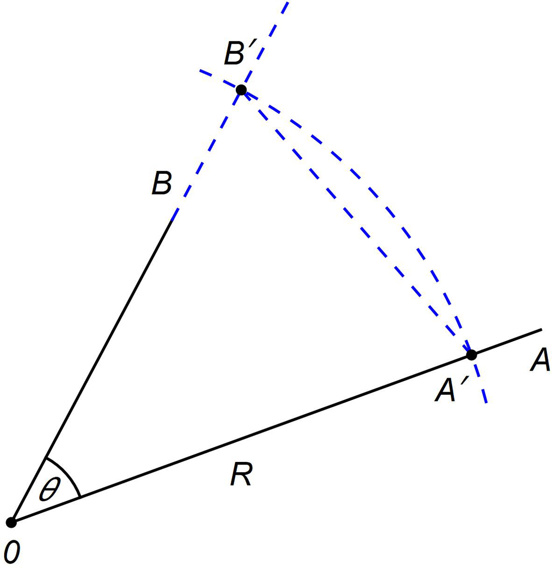
The basic principle is illustrated in Figure 4. To measure ∠A0B, a drawing compass is set to 60° on the chord (CH) scale. This is equal to the radius, R, of the reference circle. An arc is drawn that intersects the lines 0A and 0B at A′ and B′, respectively. Dividers are set on A′ and B′ and the length transferred to the chord (CH) scale from which ∠A0B can be read. For obtuse angles, the supplement, 180°−θ, is measured. Drawing a required angle is roughly the inverse of this procedure.
Measuring ∠A0B or drawing the angle θ from the chord A′B′ on the reference circle.

4.2. Navigation
Bowditch (Reference Bowditch1851, p. 18) describes, in great detail, the geometric construction of the Plane Scale and provides a reduced version of Figure 2, but then makes very limited use of it elsewhere. Two examples are given under the heading ‘BY PROJECTION’. On page 54, the Plane Scale is simply used to draw an angle of 5 compass points (56¼°) in a plane sailing problem. On page 64, the sine scale is used to reduce nautical miles at the equator to nautical miles at a specified latitude by geometric construction in a parallel sailing problem. A second solution is also given in which the Plane Scale is used to draw an angle.
4.3. Spherical trigonometry
To treat problems in spherical trigonometry, the surface of the sphere is mapped to the plane by stereographic projection, the properties of which are summarised in Appendix A. All circles on the sphere map to circles on the plane but, in general, the projection of a circle’s pole is not the centre of the projected circle on the plane. A suite of geometric constructions is then available to measure spherical angles and arc lengths (see Appendix B). In many cases, the use of the Plane Scale replaces the geometric constructions and streamlines the process of finding solutions.
It will be assumed here that the sphere has a radius, R, which is the same as the radius of the primitive circle and the reference circle used to construct the Plane Scale.
Figure 5 shows the arc of a great circle ABC projected stereographically onto the plane. It cuts the primitive circle, ADCE, at diametrically opposite points A and C. Its centre and poles are colinear with the centre of the primitive circle, 0. If the pole of a great circle on the sphere is at polar distance, d, then on the plane, its radius and the distances of its centre and poles from the centre of the primitive circle are as given below.
 $${\rm{Radius:}}\,\,\,\,r = R\sec d$$
 $${\rm{Distance \;of\; centre:}}\,\,\,\,\,\,\,\,\,\,c = R\tan d$$
 $${\rm{Distance\; of\; pole:}}\,\,\,\,\,\,\,p = R\tan {d \over 2}$$
 $${\rm{Distance \;of\; opposite\; pole:}}\,\,\,\,\,\,\,\,\,p' = R\tan \left( {{{180^\circ - d} \over 2}} \right)$$
Plot showing positions of the centre, c, and poles, p, p′, of the great circle ABC of radius, r, on the plane. The primitive circle ADCE has radius R.

The secant (SEC), tangent (TA) and semi-tangent (S·T) scales are therefore ideally suited for plotting these positions when any one of the others is known.
5. Great circle sailing
Collins (Reference Collins1659, p. 80) demonstrates the graphical solution of a great circle sailing problem using stereographic projection. As noted earlier, he ‘shuns’ the use of the secant, tangent and semi-tangent scales, instead obtaining these trigonometric functions by geometric construction each time they are needed. One such construction is shown in Figure 6. The reader is instructed to set the dividers to the angle θ on the Line of Chords and prick this off twice from the point S on the primitive circle. Setting the dividers on 0P gives R tan θ and NP gives R sec θ.
Geometric construction used by Collins (Reference Collins1659) to obtain the lengths R tan θ and R sec θ graphically.

Collins’ solution to the great circle sailing problem will be reproduced here but making full use of the secant, tangent and semi-tangent scales, which simplifies and shortens it considerably. The underlying principles will also be explained. The problem is stated in its original form as:
‘Let there be two places , the one is 50d North Latitude, as is the Lizard, the other is 36d 00′ South Latitude, and let the difference of Longitude between them be 68d 30′.
Firſt, it is required to draw the great Arch in that Projection, and then to finde the greateſt Latitude or Obliquity thereof, and the Diſtance in the ſaid Arch, and thirdly to finde what Latitude it paſſeth through at 10d difference of Longitude from the place in South Latitude.’
To solve this problem, Collins works in an equatorial stereographic projection. His results are quoted to an unrealistic 1 arc minute of accuracy. As is standard, the solution begins by drawing the primitive circle ÆNQS with radius, R, taken from the 60° point on the chord (CH) scale. The geometric construction is shown in Figure 7 with the line ÆQ representing the equator.
Plotting the great circle sailing initial point, T, its diametric opposite, A, and the Lizard, L, under equatorial stereographic projection. The great circle drawn through these three points has its centre at V.

Prick off the projection of the point at 36°S from Æ at T on the limb of the primitive circle. This can be done since, as indicated in Appendix A, the intersections of the projected parallels with the primitive circle are uniformly spaced around its circumference. Mark the point A diametrically opposite T. Points A and T lie on the required great circle and the next step is to find a third point which will then allow the circle to be drawn. This procedure is analogous to drawing the circles representing parallels and meridians on a Wulff net (Figure A3). Prick off the point Z on the primitive circle’s limb that is 50° from Æ. This point lies on the same parallel of latitude as the Lizard. Under equatorial stereographic projection, that parallel has a radius R tan d, where d is the polar distance, which in this case is 40°; the complement of the Lizard’s latitude. Set the radius from 40° on the tangent scale and draw an arc centred on Z that cuts the extended SN axis at G. With the same radius, draw the parallel as a circle centred on G. Similarly, the meridian at a longitude difference of 68° 30′ from T is found by drawing an arc of radius R sec(68.5°) centred on points N and/or S that crosses the extended equator at E. With the same radius, draw the meridian circle NLS centred at E. The Lizard’s projected position, L, is at the intersection of the circles representing the parallel and meridian. The great circle can now be drawn through the points T, L and A by standard methods which find the centre, V.
The great circle’s centre and radius are now known. Its obliquity or inclination to the equator can be found by setting the radius on the dividers and reading the angle on the secant (SEC) scale. This is also the maximum latitude that it reaches, which in this case is 59° 56′ in agreement with Collins.
Plotting a great circle on a Mercator chart requires finding its latitude at regular intervals in longitude. To do this, Collins uses the construction shown in Figure 8. To obtain the latitude at 10° longitude difference from T, set the dividers to 10° on the semi-tangent (S·T) scale and prick off the point x lying at that distance from C on the line CQ. Do the same for 10° on the tangent (TA) scale and prick off the point z. These points are the pole and centre respectively of the circle representing the meridian at a longitude difference of 10° from T. Draw that meridian centred on z and passing through N and S. It intersects the great circle at f. Reduce f to the point m on the primitive circle by drawing a line through f from the pole x (see Appendix B.5). The required latitude of 23° 55′S is found by measuring ∠ÆCm. Collins gives 22° 8′S.
Plotting the point f on the great circle at 10° longitude difference from the initial point, T. The point f is reduced to the primitive circle at m and its latitude ∠ÆCm measured.

The method used to find the great-circle distance from the initial point to the Lizard is illustrated in Figure 9 (see Appendix B.5). As the centre of the great circle, V, is known, its pole, r, can be quickly found. Set the dividers to CV and read the angle off the tangent (TA) scale. Set the dividers to this angle on the semi-tangent (S·T) scale and prick off the point r along the line CV. Reduce the point L to the primitive circle at t by drawing a line from the pole r through L. The required great-circle distance is found from ∠TCt to be 105° 03′. Collins gives 105° 53′.
Reducing the Lizard, L, to the primitive circle to obtain the great-circle distance by measuring ∠TCt.

Arguably, Collins’ great circle sailing problem can be more easily solved with a polar stereographic projection as demonstrated in Figure 10.
Collins’ complete great circle sailing problem solved by means of a south polar stereographic projection.

This shows a south polar stereographic projection with the north pole, N, at the centre of the primitive circle. Meridians are straight lines. The initial point at latitude 36°S, T, lies at a distance R tan(d/2), where d = 126° is its north polar distance. The projection of the Lizard, L, can be similarly plotted. The point A, diametrically opposite T, can be found using the Plane Scale or by geometric construction described in Appendix B.2. Drawing a circle through the three points T, L and A yields its centre, V, from which its inclination to the equator and maximum latitude can be immediately determined by Equation (1) and the secant (SEC) scale on the Plane Scale.
Draw a line at a 10° angle to NT and find the point f where it intersects the great circle. This is the point at a difference in longitude of 10° from T. Set the dividers on N and f and use the semi-tangent (S·T) scale to find its polar distance and hence latitude.
From the known position of the great circle’s centre, find the position of the pole, r. From r, reduce L to t and T to t′ on the primitive circle (see Appendix B.5). The great-circle distance is ∠t′Nt.
The initial course to steer is the angle that the great circle makes with the meridian, NT, at T. This is the complement of ∠NTV which yields N38.3°E.
Acknowledgements
The author wishes to thank Lars Bergman for his meticulous reading of the manuscript and Robert H. van Gent for providing additional reference material.
Appendix A
Properties of stereographic projection
Figure A1 shows the stereographic projection of a point P on the surface of a sphere of radius R from the point N to a point P′ on the equatorial plane. If the centre of the sphere is the point 0, then 0N is normal to the plane. The intersection of the surface of the sphere with the plane is known as the primitive circle.
Stereographic projection of the point P on the sphere from the north pole, N, on the point P′ on the plane.

Stereographic projection is conformal or angle-preserving. All circles on the sphere map to circles on the plane but, in general, the projection of a circle’s pole is not the centre of the projected circle on the plane.
In principle, the projection point can be any point on the sphere but is normally one of the poles, (polar stereographic projection) or a point on the equator (equatorial stereographic projection).
Suppose the usual coordinate grid of latitude and longitude exists on the surface of the sphere. Figure A2 shows the meridians of longitude and parallels of latitude plotted at 10° intervals under north polar stereographic projection. Although it extends beyond it, the stereographic projection is only shown inside the primitive circle which, in this case, is the projection of the equator with the projection of the south pole, S, at its centre. Meridians map to straight lines radiating from the pole. The parallel at latitude, L, lies a polar distance, d = 90°+L and is projected onto a circle with radius r = R tan(d/2).
Latitude and longitude grid under stereographic projection from the north pole

Figure A3 shows an equatorial stereographic projection from a point on the equator. Both meridians and parallels are plotted at 10° intervals. Again, although stereographic projection maps the entire surface of the sphere, with the exception of the projection point, onto the plane, only one hemisphere is shown here. The figure is analogous to the Wulff net or stereonet used in crystallography and other applications. The grid lines are all arcs of circles and, because stereographic projection is conformal, they intersect at right angles. If the radius of the primitive circle is R, then the projected parallels are circles of radius r = R tan d with centres at a distance c = R sec d from the origin on the vertical axis. Here, d is again the parallel’s polar distance. Meridians are circles of radius r = R sec Δλ centred a distance c = R tan Δλ from the origin on the horizontal axis where Δλ is the difference in longitude from the meridian at the outer edge of the figure. The intersections of the projected parallels with the primitive circle are uniformly spaced around the circumference.
Latitude and Longitude grid under stereographic projection from a point on the equator

Identifying the sphere with the Riemann Sphere and points on the plane under stereographic projection with complex numbers has been shown to have applications in navigation and astronomy (Stuart, Reference Stuart1984, Reference Stuart2009a, Reference Stuart2009b, Reference Stuart2017).
Appendix B
This appendix describes geometric constructions that can be used to solve problems in spherical trigonometry graphically. Many of the constructions can be simplified when the points involved lie on or at the centre of the primitive circle. These will not be discussed, but can be found from Bion (Reference Bion1723).
Alternative direct procedures using the Plane Scale are also given.
B.1 Finding the pole of a great circle
Figure B1 shows a stereographic projection of the arc ABC of a great circle. Note that any great circle will cut the primitive circle at diametrically opposite points. Draw the diameter AC and its perpendicular DE. Draw a straight line through the points A and B intersecting the primitive circle at F. Form the right angle F0h and connect A and h with a straight line. The intersection of the line hA with DE is the projection of the required pole, P.
Geometric construction for finding the pole, P, of the great circle ABC.

To understand why this construction works, consider the primitive circle ADCE as being a section through a sphere and make a stereographic projection from the point A onto a plane perpendicular to the page passing through DE. Then, B is the projection of a point F on the great circle and P is the projection of a point h which is 90° away from it and is therefore the pole.
Plane Scale
If the centre of the great circle, V, is known, then set 0V on the dividers and read the angle off the tangent (TA) scale. Set that angle on the dividers from the semi-tangent (S·T) scale and prick off 0P to find the pole.
B.2 Finding the diametrically opposite point
Let P be the point on the plane whose diametrical opposite is required. Draw the line ED through P and 0 and extend it outside of the primitive circle. Draw the perpendicular diameter AC. Draw the line CP and extend it to meet the primitive circle at M. Draw a line starting at C at right angles to the line CM and intersecting the extended line ED at P′ which is the required point. The right angle may be most easily constructed by drawing the diameter M0M′.
The explanation behind this construction is as follows. As in the previous section, in Figure B2, consider the primitive circle ADCE as being a section through a sphere and make a stereographic projection from the point C onto a plane perpendicular to the page passing through DE. The points P and P′ on the plane are the projections of M and M′ which are diametrically opposites on the sphere.
Geometric construction for finding the point P′ that is diametrically opposite the point P. If P is the pole of a great circle, then P′ is the opposite pole.

Plane Scale
The point P′ can be obtained more directly using the Plane Scale. If the distance 0P is R tan(d/2), then the distance 0P′is R tan ((180°− d)/2). Set the dividers to 0P and lay them on the semi-tangent (S·T) scale noting the angle. Set the dividers to the supplement of this angle on the semi-tangent (S·T) scale and prick off 0P′.
B.3 Drawing a great circle through two points
Suppose two points on the plane a and b are given. The projection of a great circle passing through them will also pass through their diametrically opposite points. The construction in Appendix B.2 can be used to find the diametrically opposite point of either a or b. With three points known to lie on the circle, its centre can be found in the usual way as the intersection of perpendicular bisectors of line segments joining pairs of points.
B.4 Drawing a great circle at right angles to another
A great circle at right angles to another must pass through both of its poles. The third point through which to draw the required great circle is arbitrary and determined by the particular problem being considered.
The great-circle distance between the points on the sphere is found by reducing their projections, a and b, on the plane to the primitive circle. The required angular distance is ∠a′0b′.

B.5 Measuring the arc length on a great circle
Suppose two points on the plane a and b are given and it is required to find their great-circle distance on the sphere. Find the pole P of the great circle ABC on which the points lie using the methods described previously. Extend the line Pa until it meets the primitive circle at a′. This is called reducing a to the primitive circle. Do likewise for the point b to find b′. The required distance on the sphere is ∠a′0b′.
B.6 Measuring the angle of intersection between two great circles
Find the poles, P and P′, of the great circles. Measure the great-circle distance between the poles as described in Appendix B.5. This is the required angle.
B.7 Drawing a small circle
Let the projected pole, P, of a small circle of radius on the sphere, r, lie at a distance R tan(d/2) from the centre, 0, of the primitive circle. The nearest point, a, and farthest point, b, on the small circle’s circumference from 0 will be at distances R tan((d−r)/2) and R tan((d+r)/2), respectively. Set the dividers on 0 and P, and read d from the semi-tangent (S·T) scale. Set the dividers to (d−r) on semi-tangent (S·T) scale, and prick off the point a from 0 along the line through 0 and P. Do the same for (d+r) and prick off the point b at distance. Points a and b are diametrically opposite on the small circle and the centre is at the mid-point of ab.
In modern navigational practice, this method could be used to plot a circle of position (COP) on a stereographic chart. If a Sun sight is taken, its geographic position (GP) is the pole and its zenith distance is the radius of a small circle of position. The standard double altitude sight problem can be solved by finding the intersection of two COPs constructed in this way.
B.8 Measuring the angle subtended at the pole of a small circle by an arc on its circumference
In Figure B4, the point P is the projection of the pole of small circle, and a and b are the projections of two points on its circumference which define the end points of an arc. The point c is the centre of the circle on the plane. Let the distance of P from the centre of the primitive circle, 0, be R tan(d/2). Set the dividers on 0 and P, and read d from the semi-tangent (S·T) scale. Use the semi-tangent (S·T) scale to draw a circle of radius R tan((180°−d)/2) centred at 0. A line from P through a cuts that circle at the point a′. The point b′ is found similarly. The angle subtended at the pole of the small circle by the arc from a to b on the small circle on the sphere is ∠a′0b′.
Geometric construction to measure the angle subtended at the pole P by an arc ab on the circumference of a small circle on the sphere.