


Introduction
Snow-accumulation changes in Antarctica are influenced by global climate changes, and, in turn, influence the sea level. Recent models of global warming predict an increase of the accumulation rate in Antarctica. This would tend to decrease sea levels and thus act in opposition to other global effects that tend to increase sea levels. Therefore, long-term changes of snow-accumulation rates are a key parameter for past-climate reconstruction. Visible stratigraphical analysis is an established technique in ice-core research to estimate annual accumulation rates (e.g. Reference BensonBenson, 1962; Reference GowGow, 1965, Reference Gow1968; Reference LangwayLangway, 1967). For the Greenland ice cores, the visible strata are used for ice-core dating. Cloudy bands are typical features in deep ice cores that have a high concentration of microparticles (dust). The microparticles are deposited in early summer, so the cloudy bands indicate former surfaces (Reference Hammer, Clausen, Dansgaard, Gundestrup, Johnsen and ReehHammer and others, 1978). Reference Shoji, Miyamoto, Kipfstuhl, Langway and HondohShoji and others (2000) found a high density of small bubbles (microbubbles) in the cloudy bands, and the microbubbles are the prime source for light scattering. These microparticles and the microbubbles in the cloudy bands will scatter light, and thus automated and quantitative analysis for strata study are possible. Reference AlleyAlley and others (1993) accurately dated the Greenland Ice Sheet Project 2 (GISP2) ice core and found that annual accumulation rates changed drastically at the Wisconsin–Holocene termination. An accurate age for the depth range of Wisconsin–Holocene termination can be estimated by annual-layer identification using a combination of visible strata observations, continuous microparticle concentration analysis and electro-conductivity measurement (Reference HammerHammer, 1980; Reference AlleyAlley and others, 1997; Reference MeeseMeese and others, 1997; Reference Ram and IllingRam and Koenig 1997). For the continuous microparticle concentration analysis of the GISP2 ice core, a liquid-type (meltwater) and solid-type (ice) technique were used. A cross-check of the two techniques shows good agreement for bubble-free ice (Reference Ram, Illing, Weber, Koenig and KaplanRam and Illing, 1994; Reference Ram and KoenigRam and others, 1995), which indicates that the light-scattering intensity from bubble-free ice is closely related to microparticle concentration. Recently, Reference Dahl-JensenDahl-Jensen and others (2002) used a line scanner apparatus to record visible strata in North Greenland Ice core Project (NorthGRIP) ice. They also identified cloudy bands as high-brightness layers in their images.
Although Greenland ice cores contain clear seasonal signals, the seasonal signals in the low-accumulation areas of inland Antarctica are not always clear. The low accumulation rates make annual layers hard to identify, so accurate dating is difficult. Nevertheless, inland Antarctic ice cores contain long-term paleoclimatic information. In general, the dating of these ice cores is calculated using an accumulation–flow model (Reference JohnsenJohnsen and Dansgaard, 1992; Reference DansgaardDansgaard and others, 1993) with some fixed date in the core, or is adjusted to agree with an ice core at another site (Reference PetitPetit and others, 1999; Reference WatanabeWatanabe, 2002; Reference WatanabeWatanabe and others, 2003a). The model uses various assumptions that introduce some potential errors into the age estimates. Consequently, a long-term dating method based on direct core measurement would be a precious tool to obtain an accurate depth–age scale.
Here, we studied the potential use of visible strata in the Dome Fuji ice core for dating purposes. The ice core was drilled in 1995/96 (Dome-F Ice Core Research Group, 1998); a visible stratification study was done in the field, and 821 cloudy bands, containing 25 tephra layers, were found in total (Reference FujiiFujii and others, 1999, 2002). However, making detailed records of the stratification was extremely difficult at the time. Nevertheless, since Reference Iizuka, Takata, Hondoh and FujiiJohnsen and others (1995) could identify cloudy bands in the Eemian, with low-microparticle-concentration ice from a Greenland ice core after it had relaxed, we assumed that it is possible to identify cloudy bands in the present Dome Fuji ice core. We therefore developed an optical scanner to detect and record visible strata. In this paper, we introduce our preliminary results on its use on Dome Fuji ice and discuss the potential of annual-layer identification using this technique.
Method
Ice cores used for the measurements had been stored at –50˚C for 6–7 years in a cold room in the Institute of Low Temperature Science (ILTS), Hokkaido University. The scanner measurements are done in an ILTS cold room at –20˚C. Figure 1 shows the optical scanning device. The equipment is similar to that used by Reference Dahl-JensenDahl-Jensen and others (2002); further details of our system are described in Reference TakataTakata and others (2003b). The light sources and mirrors are located below the ice. We use two rows of 24 white light-emitting diodes (LEDs), 100mm wide, as a light source because they have a low heat generation, high stability, a long lifetime and are low-cost. The light sources and charge-coupled device (CCD) camera are mounted on a moving stage and moved along the ice-core sample during the measurements. In polar ice cores, light scattering occurs mainly at air inclusions and microparticles. The distribution of scattered light intensity from the ice sample is measured using a CCD camera, and the brightness intensity of each pixel is recorded by a digital video recorder. The positions of the lights and mirrors are adjusted to direct light through the center of the observation area. The CCD is focused on the top surface of the ice. After a measurement, the digital video images are captured by a PC, and a scanned image of the whole ice core is produced using special original image analysis software.
The optical scanner set-up. The ice-core sample is fixed on a stage, and the optical devices move along the core sample.
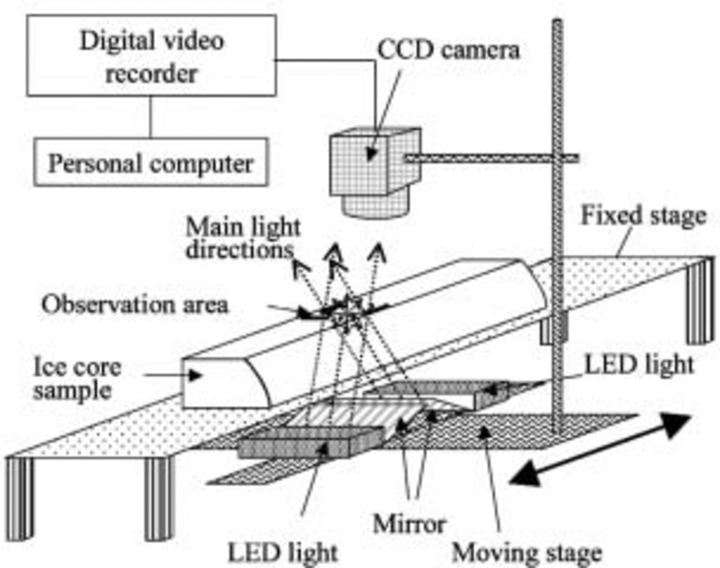
The ice sample has two parallel surfaces as shown in Figure 1. Both surfaces are smoothed with a microtome just before the measurements. Measurement resolution is adjusted to 0.037 mmpixel–1. The scanning speed is 4.5 mms–1; thus, in contrast to the relatively long time for sample preparation, each 50cm long ice-core sample is measured within 2 min.
Results
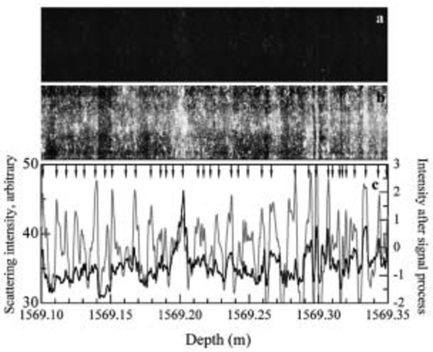
To illustrate the method, we describe measurements at various depths in the Dome Fuji ice core. Figure 2 shows the result for depth range 1569.10–1569.35m in the measurement and analysis range 1569.00–1569.50 m, in a bubble-free zone with an age corresponding to 112 kyr BP according to the depth–age relationship for Dome Fuji proposed by Reference WatanabeWatanabe and others (2003a). Figure 2a shows a scanner image, and Figure 2b shows an enhanced intensity image of Figure 2a. The enhanced intensity image is obtained from the original by using the histogram equalization process. In the images, the bright regions are strong scattering regions and the dark regions are weak scattering regions. The contrast in Figure 2a is smaller than in a north-central Greenland ice core measured with our prototype equipment (Reference Takata, Shoji, Miyamoto and ShimoharaTakata and others, 2003a), probably due to the difference of microparticle concentration levels (Reference Ruth, Wagenbach, Bigler, Steffensen, Röthlisberger and MillerRuth and others, 2002; Reference WatanabeWatanabe 2002). Even though no visible layers were found in the initial visual examination of the ice core, the present ice core contains a large number of layers (Fig. 2b). Although manual identification of layers is possible using Figure 2b, the results would depend on the person making the observations.We therefore developed a numerical method. As the first step, the scattering intensity profiles were calculated. The scattering intensity is the average intensity of same-depth pixels in Figure 2a, which is shown as the black line in Figure 2c. The scattering intensity profile fluctuates in phase with the layers in Figure 2a. Accurate layer identification, however, is difficult because the fluctuation amplitudes are small. As the second step, we processed the signal and obtained the profile shown as the gray line in Figure 2c. The signal-processing method and layer identification technique are described below. The intensity profile after the signal shows large amplitude fluctuations and thus has the potential for accurate layer identification.
Scanning measurements on 1569 m ice. (a) Original image. (b) Enhanced intensity image of (a). (c) The scattering intensities averaged over points at the same depth. The black line is the profile from the original image. The gray line is the profile processed to include only cycles between 0.6 and 12 mm. The vertical direction in (a) and (b) is stretched to show the structure. The intensity level is 256, and the absolute value of the intensity is arbitrary because it depends on the measurement conditions such as incident light intensity and aperture of the CCD lens. Arrows indicate layer boundaries determined by the signal-processing technique.
A deeper, bubble-free region of ice (1818.48–1818.73 m, in the measurement range 1818.46–1818.98 m) containing a volcanic tephra layer is plotted in Figure 3. The age of this ice is estimated to be the termination from marine isotope stage 6–5.5 and 135 kyr BP. The brightest band, at 1818.51 m, is a volcanic tephra layer, confirmed by Reference FujiiFujii and others (1999), with a value that exceeds the scale range in the figure. Many identified layers are also found as bright bands in the images and peaks of the intensity profiles.
Scanning measurements on 1818m ice. Measurement conditions are the same as in Figure 2. A known volcanic ash layer is located at 1818.51 m. (a–c) are analagous to Figure 2a–c except the signal-processed profile in (c) was obtained using intensities from cycles between 0.8 and 16mm. Horizontal lines in (b) are scratches from the microtome, which occur despite frequent changes of the microtome blade.

Ice from an even deeper, bubble-free zone (1899.10– 1899.35 m, in the measurement range 1899.00–1899.50 m) is shown in Figure 4. This ice has an estimated age of 151 kyr BP. The layers are clearer in this figure than in Figures 2 and 3 because the ice has the highest microparticle concentration of the three samples (Reference WatanabeWatanabe, 2002).
Scanning measurements on 1899 m ice. Measurement conditions are the same as in Figures 2 and 3. (a–c) are analogous to Figures 2a–c and 3a–c except the signal-processed profile in (c) was obtained using intensities from cycles between 1 and 10 mm. plots, but the decreases in trend toward longer wavelength are different. In addition, Figure 6a has peaks at 13–20 mm.

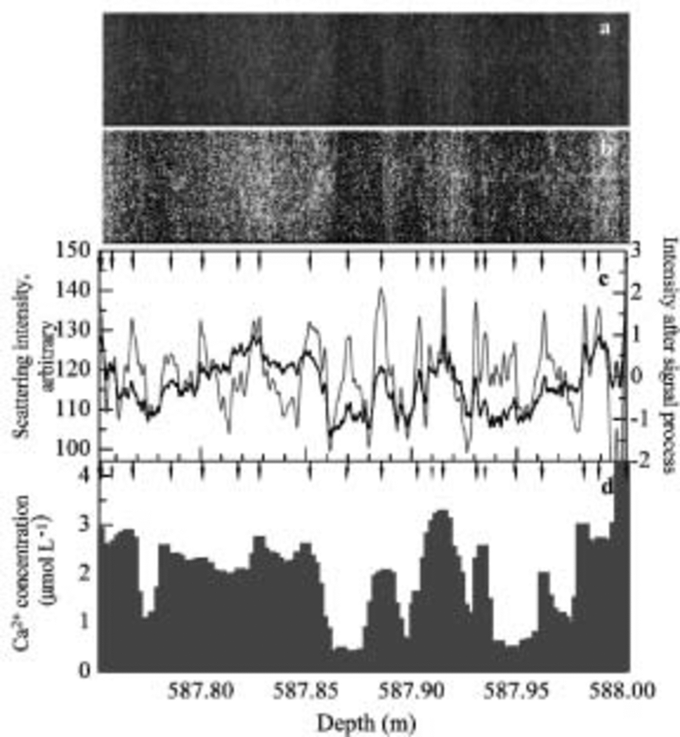
A relatively shallow region with air bubbles is analyzed in Figure 5. In this depth range (587.75–588.00 m) the ice has an estimated age of 25 kyr BP in the Last Glacial Maximum period. Because the original profiles have small fluctuations due to the air bubbles, we smoothed the profiles in Figure 5c by averaging over 1 mm sections. On the same depth sample, Reference Iizuka, Takata, Hondoh and FujiiIizuka and others (2004) also did ion-chromatography analysis with 2 mm resolution. The Ca2+ concentration from this analysis is shown in Figure 5d and described below.
Scanning measurements on 587 m ice. (a–c) are analogous to Figures 2a–c and 3a–c except the signal-processed profile in (c) was obtained using intensities from cycles between 1.5 and 30 mm. (d) Calcium concentration profile from ion-chromatography measurements by Reference Iizuka, Takata, Hondoh and FujiiIizuka and others (2004). Gray arrows indicate that layer boundaries determined by a signal-processing technique disagree with the Ca2+ peak.
The Possibility of Annual-Layer Identification
Signal processing of intensity profile and layer-boundary identification
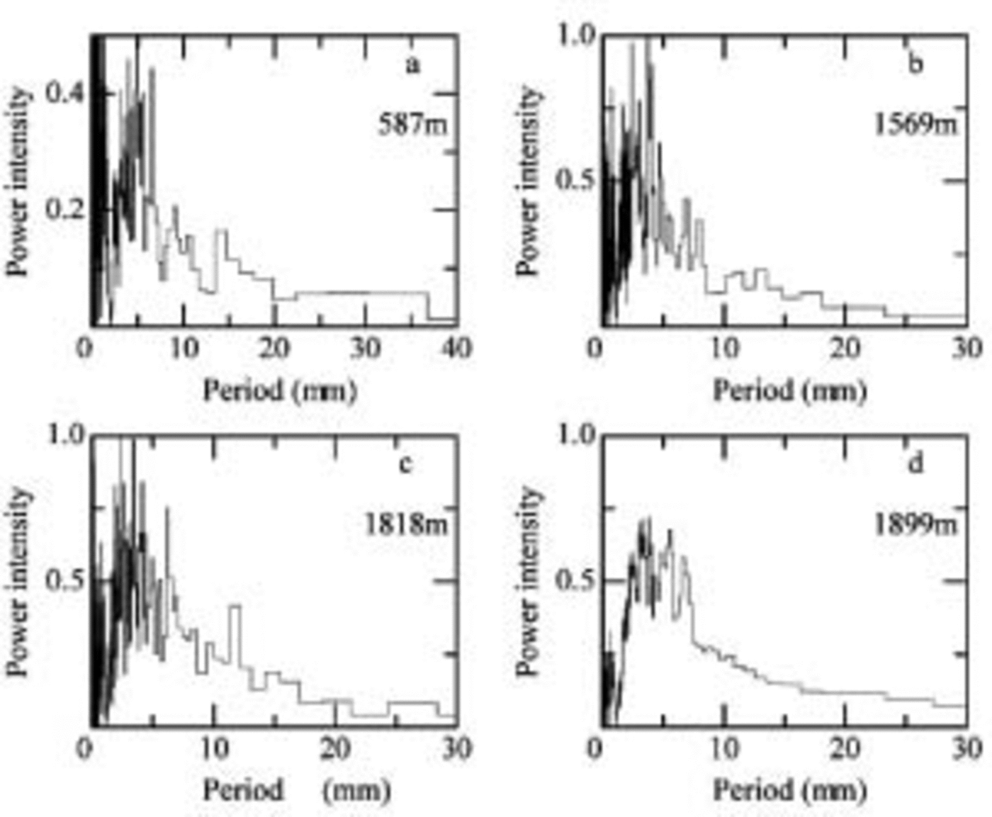
We used signal-processing methods to identify the layers more clearly. Before the signal processing, we investigated periodicity features of the scattering intensity profile using fast Fourier transform (FFT) analysis with a Hanning-type window. Running means of 2 mm for the bubbly ice sample (589m ice) and 1 mm for bubble-free ice samples (1569, 1818 and 1899 m ice) and normalized profiles of the enhanced images are used for the FFT analysis. Figure 6a–d shows a plot of power intensity vs period for 578, 1569, 1818 and 1899 m ice, respectively. Power intensities of three-point averages are shown in the figure. Because the present annual mean accumulation rate at the Dome Fuji site is approximately 30 mmw.e. (Dome-F Ice Core Research Group, 1998) and the layer thickness should decrease with increasing depth due to the deformation of ice under overburden pressure, we only plot the power intensities in the range 0–30 mm. The power-intensity distributions vary from sample to sample. Peaks appear within 0–10mm in all
Power intensity of intensity profile of the enhanced intensity images. The samples are from 578 m ice (a), 1569 m ice (b), 1818 m ice (c), and 1899 m ice (d). Various signal-processing methods were used as described in the text.
In order to estimate the modeled annual-layer thicknesses, we used the accumulation–flow model of Johnsen and Dansgaard (1992). The following parameters were used: H= 2990 m, h = 1400 m, f b = 0.25 (ratio between strain rates at top of sliding layer and at the surface), and accumulation = 0.028 exp (δ18O + 55.0) × 0.08 m ice equivalent a–1 (personal communication from S. Reference Johnsen, Dansgaard, Bard and BroeckerJohnsen, 2002). Reference Watanabe, Jouzel, Johnsen, Parrenin, Shoji and YoshidaWatanabe (2003b) also calculated the annual-layer thickness and found values close to the estimated thickness using different parameters from S. Johnsen. The modeled annual-layer thicknesses are 7–8 mm at 1569m depth, 5–6mm at 1818 m, 5 mm at 1899 m, and 14–15mm at 587m depth.
The results of the FFT analysis show a broad peak at the modeled annual-layer thickness. This supports the estimates and indicates that our scanning method can be used to identify annual layers. In addition to the signal that we assign to the annual layers, the scattering intensity profile has higher- and lower-frequency signals. These high- and low-frequency signals make it difficult to identify annual-layer boundaries, so these signals were cut from the scattering profiles. The high frequencies that had wavelengths less than one-tenth of the average annual-layer thickness were assumed to be too thin to be layer thicknesses, so we classified them as noise and cut the frequency signals from the profile. Also, frequencies with longer wavelengths more than twice the average annual-layer thickness do not have an annual signal, so we also cut these from the profile. Support for our rejection of these high and low frequencies is as follows: The spatial resolution of the intensity profiles is high, 26.75 points mm–1, and 10 data points a–1 are acceptable to identify annual boundaries. The high-resolution data might make high-frequency noise. And the results of annual snow-stake measurements in the Dome Fuji area assembled during 1992–2001 by Reference Kamiyama, Furukawa, Maeno, Kishi and KanaoKamiyama and others (1994), Reference Motoyama, Enomoto, Miyahara and KoikeMotoyama and others, (1995, Reference Motoyama, Kawamura, Kanao, Hirasawa, Kaneto and Yamanouchi1999, Reference Motoyama2002), Reference ShiraiwaShiraiwa and others (1996), Reference AzumaAzuma and others (1997), Reference Fujita, Kawada and FujiiFujita and others (1998) and Reference FurukawaFurukawa and others (2002) show that an accumulation thickness of more than double the annual average thickness occurs only in 7% of the years. An accumulation rate study at South Pole during 1760–1942 (Reference Hogan and GowHogan and Gow, 1997) also shows that accumulation thickness of more than double the annual average thickness is rare.
We decided to use a wavelength range from one-tenth of to twice the annual average thickness for signal processing. Signal-processed profiles might be expected to be affected by the center wavelength of the range, but this is not so. In a case study, uniform power intensities were assumed and signal-processed profiles were obtained. We found that the profiles were strongly affected by the lowest cut-off frequency. We used twice the annual-layer thickness for the limit of lowest frequency; thus, the intensity profiles after signal processing were affected by twice the annual-layer thickness and not affected by annual-layer thickness if the power intensities were uniform.
This signal processing requires an estimate of the annual thickness. Unfortunately, we cannot determine this from Figure 6. Therefore, we used the modeled annual-layer thickness. As mentioned previously, the estimated annual-layer thicknesses are 7–8 mm at 1569m depth, 5–6mm at 1818 m, 5mm at 1899 m, and 14–15mm at 587 m depth. Therefore the wavelength ranges used for the signal processing were 0.8–16 mm at 1569m depth, 0.6–1.2mm at 1818 m, 0.5–10mm at 1889 m, and 1.5–30mm at 587 m depth. After signal processing, we normalized the profile. The profiles are shown in Figures 2c, 3c, 4c and 5c as gray lines with the scale on the right side. The amplitude of the profiles is greater than those from the scattering intensity profiles. The peak locations in the signal-processed profile also correspond to those in the original scattering intensity profile.
Using the signal-processed profile, we tried to identify layer boundaries. We began by using a fixed threshold value for the top and bottom peaks, but too few or too many layer boundaries were identified, so we abandoned this method. Then we identified a layer boundary if it met the following four conditions:
-
1. the peak is above zero
-
2. the minimum between two layer boundaries is below zero
-
3. the peak height minus the nearest minimum exceeds 0.8
-
4. the peak height is more than 0.5 above another nearby minimum.
The layer thickness of the identified layers is larger than 1 mm (26 pixels). The probability that 26 consecutive points have values satisfying the above conditions is <0.0005 on a normalized random profile. This estimate indicates that our method is unlikely to assign a layer boundary incorrectly, and that layer identification using the four conditions is acceptable for use here. The resulting layer boundaries are marked with arrows in Figures 2c, 3c, 4c and 5c. Inspection of the arrows and the enhanced intensity images (Fig. 2b, 3b, 4b and 5b) shows that the method provides reasonable estimates of the layer boundaries. A few peaks are critical to identify layer boundaries, but the identified layers have a dark–bright change in the enhanced images, and peaks appear on the scattering intensity profile.
In Figure 2c, there are 35 peaks in 250 mm, so the average layer thickness is 7.1 mm, which compares well to the model prediction of 7–8 mm. In Figure 3, the average is 6.3 mm vs the model’s 6–7mm; Figure 4 has an average layer thickness of 6.0 mm, which is reasonably close to the model prediction of 5 mm; and Figure 5 has an average of 12.5 mm vs the model’s 14–15 mm. Thus, each layer thickness obtained with this method is close to the estimated annual-layer thickness from the depth–age model.
Chemical constituent and annual-layer identification
We compared the scattering intensity with chemical constituents in the 587 m sample. Calcium was selected for comparison for the following reasons: Reference Iizuka, Takata, Hondoh and FujiiJohnsen and others (1995) suggest that visible cloudy bands consist of microbubbles formed around microparticles after the retrieval of the ice core from great depth; calcium concentration is strongly correlated with microparticle concentration in Greenland ice cores (Reference SteffensenSteffensen, 1997; Reference Ruth, Wagenbach, Bigler, Steffensen, Röthlisberger and MillerRuth and others, 2002); and the calcium concentration profile in the Dome Fuji ice core has fluctuations similar to those in the microparticle profile (Reference WatanabeWatanabe, 2002). The calcium concentration profile in Figure 5 has similarities to the profiles obtained by the scanner measurement, but the correlation coefficient of the two profiles is only 0.531. For reference, chloride concentration was also compared with the scattering intensity, but the profile shows some different fluctuations, so the correlation coefficient is lower than for calcium. We selected the peak position on the calcium profile where one of the following conditions is satisfied: (1) an obvious large peak, (2) a shoulder region after a large concentration, or (3) small peaks for which two or more concentrations are larger than those in the nearby region. In Figure 5d, the solid arrows mark calcium peaks that correspond to layer boundaries in Figure 5c, whereas the dashed arrows mark peaks that are not at layer boundaries. The layer boundaries agree with 18 out of 21 Ca2+ peaks, and only two relatively small calcium peaks, at 587.815 and 587.975 m, disagree with the layer boundaries. Thus, the peak locations in the calcium concentration profile agree well with those from the scattering measurements. The three layer peaks that do not appear in the Ca2+ profile are close to neighboring peaks compared with other peak intervals and thus represent relatively small layer thicknesses compared to the average of 12.5 mm obtained by this method. If these 3 boundaries are ignored and the 18 remaining layers are assumed to be layer boundaries, the layer thickness is 13.2 mm, an increase of 0.7 mm. We also compared the Ca2+ concentration peaks with the scattering intensity peaks on another 250 mm long section and found good agreement. Finally, the Dome-F Ice Core Research Group (1998) suggest that the calcium concentration increased in early summer and decreased in winter, based on 1 year’s results, which supports the above findings.
However, air bubbles in this sample can also be a source of light scattering. We consider the influence of air bubbles on annual-layer identification to be small, although we have no evidence of air-bubble distribution in the sample. Because cloudy layers were not detected by visible observation in the field, however, the present sample contains conspicuous layers. For example, conspicuous cloudy layers at 587.88–587.89 and 587.98–587.90m are easy to identify in the present sample as shown in Figure 5a, but were not found in the field measurement. Therefore the main scattering sources contributing to the scattering intensity fluctuation should be microbubbles, related with calcium and microparticles. Air-bubble measurements by Sugisaki (2002) show small fluctuations of bubble number close to this depth, supporting our consideration. On the other hand, Reference NaritaNarita and others (2003) suggest large fluctuations in the number density of air bubbles. Therefore we may be better off investigating the distribution of scattering sources and their contribution to scattering intensity for a future study.
We have argued that the peaks of the signal-processed profile are likely to be useful for detecting annual-layer boundaries in Dome Fuji ice cores. Although the calcium and microparticle variations at this site are poorly known now, we expect these to show a seasonal variation as well, which would be useful for annual-layer identification at Dome Fuji. We now give a physical reason why annual layers correlate with the scattering profile. The seasonal microparticle variation is recognized in Greenland ice cores as cloudy bands (Reference HammerHammer and others, 1978). Optical techniques are used for microparticle concentration measurements and cloudy-band recording in Greenland ice cores (Reference NaritaRam and Koenig, 1997; Reference Dahl-JensenDahl-Jensen and others, 2002). The calcium concentration also correlates well with the microparticle concentration in central Greenland (Reference Takata, Shoji, Miyamoto and ShimoharaSteffensen, 1997; Reference Ruth, Wagenbach, Bigler, Steffensen, Röthlisberger and MillerRuth and others, 2002) and in a Dome Fuji ice core (Reference WatanabeWatanabe, 2002). The insoluble microparticles in polar ice do not diffuse (Reference HammerHammer, 1977; Reference Johnsen, Clausen, Dansgaard, Gundestrup, Hammer and TauberJohnsen, 1977), so the annual insoluble microparticle maximum should be preserved for a long time in the ice. In support of this predicted annual microparticle signal, we found that (1) the average layer thickness is close to the estimated value and (2) the layer boundaries agree well with the calcium peaks. Thus, the preliminary analyses presented here support the use of the processed intensity profile as an indicator of annual boundaries.
Concluding Remarks
We developed an optical scanner for ice-core studies and used it on a Dome Fuji ice core. The scanner enabled us to make preliminary estimates of the annual layers even though we could not identify the layers with initial visible stratigraphy analysis in the field. We also identified a volcanic layer and many cloudy bands at all depths. We discussed the possibility of identifying annual layers in the Dome Fuji ice core using the strata, and show that the method has the potential to identify annual layers. However, before this strata method becomes an accurate dating tool, we should address the following two points.
-
1. Present and past variations of microparticle concentrations at Dome Fuji should be investigated, and we need to check that the dust signal shows a seasonal cycle.
-
2. This signal-processing and layer-boundary-identification method using scanner images should be improved.
When these requirements are met, the scanning method of strata dating with continuous measurement of the samples will provide an accurate depth–age scale for Dome Fuji and other inland Antarctic ice cores.
Acknowledgements
We thank the Dome Fuji drilling team and all the participants in the field. We also thank. T. Gow and an anonymous reviewer for their valuable comments and suggestions. This study was supported by the Grant-in-Aid for Creative Scientific Research, grant No. 14GS0202.



