4.1. Mean sphere velocities and fluid forces

Figure 5(a) shows the variation of the non-dimensional asymptotic mean velocity $\bar {u}_s^*$ of the sphere, as a function of the modified Reynolds number $Re^*$ and for various density ratios. The values are located around 1, which means that the velocity scale used for the non-dimensionalisation is indeed of the order of the terminal sphere velocity. The line passing through the data corresponds to the speed obtained from (2.17) using force and torque coefficients from the uniform rolling case. Clearly, $\bar {u}_s^*$ increases with $Re^*$, which according to (2.17) and (2.18) corresponds to a decrease of the effective drag coefficient. The Reynolds number based on the asymptotic velocity ($\overline {Re}$) is shown in figure 5(b). It varies almost linearly with $Re^*$, and the two are approximately equal for $Re^*\approx 100$. The density ratio $\beta$, which was varied over two orders of magnitude, has a negligible effect on the mean sphere velocity in the asymptotic state for $\beta > 1$. However, for lower mass ratios, there is some deviation as cross-slope motion becomes more substantial. Approximate quadratic fits relating $\overline {Re}$ and $Re^*$ are

(4.1)\begin{equation} \overline{Re} \approx -27.37 + 1.197\,Re^* + 0.001458\,({Re^*})^2 \end{equation}

and

(4.2)\begin{equation} Re^* \approx 23.31 + 0.7553\,\overline{Re} - 0.0003783\, (\overline{Re})^2. \end{equation}

While these relationships are for gap ratio $G/d = 0.005$, (2.17), (4.6), (4.7) and (4.8) can be used to extend them to any gap ratio. For example, figures 5(a,b) show predictions for gap ratio $G/d = 5 \times 10^{-6}$, for $\bar {u}^*_s$ and $\overline {Re}$ against $Re^*$, which approximately match the experimental variations.

Figure 5.

Dependence of (a) the mean asymptotic sphere velocity $\bar {u}_s^*$ and (b) the corresponding Reynolds number $\overline {Re}$ on $Re^*$, as determined from numerical simulations with gap ratio $G/d=0.005$. The grey symbols represent experimental measurements. The discrepancy with the numerical results is discussed in § 4.5. On this point, the dotted lines correspond to predictions based on (2.17), (4.2), (4.6), (4.7) and (4.8) for gap ratio $G/d=5\times 10^{-6}$, showing an approximate match to the experimental data.

Figure 5(a) also contains the results obtained in the experimental study, using different spheres. In addition to a noticeable scatter of the data, the experiments yield significantly lower sphere velocities throughout the considered Reynolds number range. This difference is due to a higher effective drag coefficient measured in the experiments, which is likely related to differences in the (effective) size of the gap between the sphere and the wall. This point is analysed further in § 4.5.

The predicted mean drag, lift and torque coefficients are shown in figure 6, as functions of the Reynolds number $\overline {Re}$, which makes it possible to compare the present results for a freely rolling sphere to those for a sphere translating at constant speed in a straight line, i.e. without flow-induced unsteady motion. The force coefficients are almost identical for the two cases. This is expected for low $\overline {Re}$, where the flow is steady and the sphere velocity is constant. It is, however, also the case at higher $\overline {Re}$ ($\gtrsim 130\unicode{x2013}150$), for which unsteady flow and sphere motion is found (see below). As for the mean sphere velocity, the dependence on the density ratio is weak. However, for very light spheres, there is measurable deviation as significant cross-slope oscillations develop. Again, this is discussed in more detail in §§ 4.3 and 4.4.

Figure 6.

Predicted mean drag and lift coefficients of the freely rolling sphere, as functions of mean Reynolds number $\overline {Re}$ for $G/d=0.005$. The solid lines represent the results for uniform rolling, i.e. rolling in a straight line at constant speed.

It should be noted that the mean lift force is negative, i.e. directed towards the wall, which is different from that observed for a rolling circular cylinder (Houdroge et al. Reference Houdroge, Leweke, Hourigan and Thompson2020). For these two cases, the flows in the gap region and their wakes are qualitatively different so the change of sign is not necessarily surprising. Perhaps a useful reference point for the expected force on a sphere is the negative lift experienced by a translating, rotating sphere such as a table tennis ball subject to top-spin. This is consistent with the predicted negative lift of a rolling sphere.

Interestingly, by considering an expansion including just linear terms in $Re$, Krishnan & Leighton (Reference Krishnan and Leighton1995) derived the asymptotic result (i.e. $G/d \rightarrow 0$) for small Reynolds number that $C_L(G/d \rightarrow 0) = 0.167$. While the drag coefficient is a strong function of gap ratio, this is not the case for the lift coefficient, which, at least for small gaps, is only weakly dependent on the gap ratio. Figure 7 shows the predicted variation of the lift coefficient for Reynolds numbers down to 0.1 for the uniform rolling case. Again, the gap ratio is $G/d=0.005$. Note that a similar variation was predicted by Lee & Balachandar (Reference Lee and Balachandar2010), who extended the work of Zeng et al. (Reference Zeng, Najjar, Balachandar and Fischer2009), although their Reynolds number resolution was lower and they restricted their predictions to the steady regime ($Re \leq 100$). Indeed, for Reynolds numbers below approximately 2.5, the lift coefficient does become positive in line with the theoretical prediction. The numerical prediction at $Re=0.1$ of $C_L = 0.173$ is only a few per cent different to that predicted analytically (0.167) by Krishnan & Leighton (Reference Krishnan and Leighton1995). The extension of the lift coefficient variation to higher Reynolds numbers may be important for particle scouring and surface cleaning applications, as discussed by Krishnan & Leighton (Reference Krishnan and Leighton1995).

Figure 7.

Predicted lift coefficient as a function of Reynolds number, $\overline {Re}$, for $G/d=0.005$ for the uniform rolling case. The dashed line shows an empirical fit for the steady Reynolds number range provided by Lee & Balachandar (Reference Lee and Balachandar2010, equation (3.15)).

Particle paths in the neighbourhood of the sphere are shown in figure 8 for $Re=1$, 10 and 100. These images show the effect of Reynolds number on the outer flow in the steady regime. The main effects of increasing Reynolds number are to decrease the boundary layer thickness at the surface of the sphere, and to break the forward–backward symmetry associated with the development of the wake, especially for $Re> 10$. The local flow in the vicinity of the gap is invariant, as will be examined in more detail in § 4.5.

Figure 8.

Particle paths in the centre plane in the neighbourhood of the cylinder as a function of Reynolds number in the steady regime. Panels (a–c) show paths for $Re = 1$, 10 and 100, respectively. The sphere is rolling to the left.

4.2. Transition to unsteady flow

Rao et al. (Reference Rao, Passaggia, Bolnot, Thompson, Leweke and Hourigan2012) investigated numerically the wake of a uniformly forward-rolling sphere and predicted that the transition from steady to unsteady, periodic flow occurs at $Re_c=139$, and that a second, mirror-symmetry-breaking transition occurs at $Re=192$. In the configuration investigated here of a sphere rolling freely under gravity, the asymptotic sphere motion and wake structure are also steady at low Reynolds number. On increasing the Reynolds number, a supercritical transition to an unsteady periodic regime is again found, with the threshold depending on the density ratio $\beta$. The critical Reynolds number can be determined from the evolution of the amplitude of a fluctuating quantity. According to the Stuart–Landau model for supercritical bifurcations (see e.g. Provansal, Mathis & Boyer Reference Provansal, Mathis and Boyer1987; Thompson & Le Gal Reference Thompson and Le Gal2004), the square of the amplitude should be proportional to the Reynolds number increment above the critical value. This value can therefore be found by extrapolating the amplitude squared to zero.

Figure 9 shows the square of the amplitude of the unsteady component of the drag coefficient, $C_D^o$, as a function of the Reynolds number $Re^*$ for various density ratios. The determination of the critical value for the uniform rolling case ($Re = 140.6$) for the current set-up is also shown in figure 9(a). This is slightly larger than but close to the value found by Rao et al. (Reference Rao, Passaggia, Bolnot, Thompson, Leweke and Hourigan2012), with the difference likely resulting from increased grid resolution around the gap. Note that for mass ratios below unity, zero cross-stream movement is enforced because otherwise the development of significant cross-stream motion affects the saturated drag coefficient values. Effectively, this allows the initial centre-plane mirror-symmetric transition to be studied in isolation. However, it does indicate that breaking of mirror symmetry occurs well below the prediction of $Re= 192$ for the uniform rolling case.

Figure 9.

Variation of the square of the amplitude of the drag fluctuation with Reynolds number, for various density ratios. Linear fits are used to determine the critical value for the onset of the unsteady regime.

Figure 10 collects the resulting critical Reynolds numbers as a function of a convenient plotting parameter $1/\sqrt {\beta }$ – chosen to spread the points so that a smooth curve joining the data points could be constructed. The onset of unsteady flow (and sphere motion) occurs at lower Reynolds numbers for lighter spheres, which is behaviour opposite to that found for a freely rolling circular cylinder (Houdroge et al. Reference Houdroge, Leweke, Hourigan and Thompson2020). This is not particularly surprising given the differences in body geometry and different flow near the gap region. For heavier spheres, e.g. $\beta =3$, the predicted transition value is slightly above that for the uniform rolling case. In the limit of very heavy spheres ($\beta \rightarrow \infty$), the threshold approaches the critical Reynolds number for uniform rolling ($Re_c=140.6$). This is expected because, as the sphere's weight is increased, it should respond increasingly less to the variation in unsteady fluid forcing as it rolls.

Figure 10.

Transition Reynolds number: $\overline {Re}_c$ as function of the inverse of the square root of the density ratio.

Insight into the effect of allowing the cylinder to oscillate on the onset of wake unsteadiness is provided by the following analysis. Taking the incompressible Navier–Stokes equations (2.2) and expanding the velocity into a time mean plus an unsteady perturbation component, $\boldsymbol {u} = \bar {\boldsymbol {u}} + \boldsymbol {u}'$, and taking the time average, gives

(4.3)\begin{equation} \bar{\boldsymbol{u}}\boldsymbol{\cdot}\boldsymbol{\nabla}\bar{\boldsymbol{u}} + \overline{\boldsymbol{u}'\boldsymbol{\cdot}\boldsymbol{\nabla} \boldsymbol{u}'} =-\frac{1}{\rho}\,\boldsymbol{\nabla} \bar{p}+\nu\,\nabla^2\bar{\boldsymbol{u}}. \end{equation}

This assumes that we are close to the steady–unsteady transition so that the perturbations are purely sinusoidal.

Subtracting this from the Navier–Stokes equations with the velocity and pressure expansions gives

(4.4)\begin{equation} \frac{\partial \boldsymbol{u}'}{\partial t} + \bar{\boldsymbol{u}}\boldsymbol{\cdot}\boldsymbol{\nabla} {\boldsymbol{u}'} + {\boldsymbol{u}'}\boldsymbol{\cdot}\boldsymbol{\nabla} \bar{\boldsymbol{u}} + {\boldsymbol{u}'}\boldsymbol{\cdot}\boldsymbol{\nabla} {\boldsymbol{u}'} - \overline{\boldsymbol{u}'\boldsymbol{\cdot}\boldsymbol{\nabla} \boldsymbol{u}'} =-\frac{1}{\rho}\,\boldsymbol{\nabla} {p}' +\nu\,\nabla^2 {\boldsymbol{u}'} - \frac{{\rm d}\boldsymbol{u}_s}{{\rm d}t}. \end{equation}

Then taking the dot product with the perturbation field, rearranging and integrating over the fluid domain (${\mathcal {V}}$) and an oscillation period ($T$) gives

(4.5) $$\begin{align} \int_t^{t+T}\iiint_{\mathcal{V}} \frac{\partial \frac{1}{2}(\boldsymbol{u}' \boldsymbol{\cdot} \boldsymbol{u}' )}{\partial t} \,{\rm d}V\,{\rm d}t &=\int_t^{t+T}\iiint_{\mathcal{V}} \boldsymbol{u}' \boldsymbol{\cdot} \left[\vphantom{\left. +\, \overline{\boldsymbol{u}'\boldsymbol{\cdot}\boldsymbol{\nabla} \boldsymbol{u}'} -\frac{1}{\rho}\,\boldsymbol{\nabla} {p}' +\nu\,\nabla^2 {\boldsymbol{u}'}\right]}- \bar{\boldsymbol{u}}\boldsymbol{\cdot}\boldsymbol{\nabla} {\boldsymbol{u}'} - {\boldsymbol{u}'}\boldsymbol{\cdot}\boldsymbol{\nabla} \bar{\boldsymbol{u}} - {\boldsymbol{u}'}\boldsymbol{\cdot}\boldsymbol{\nabla} {\boldsymbol{u}'}\right.\nonumber\\ &\quad\left. +\, \overline{\boldsymbol{u}'\boldsymbol{\cdot}\boldsymbol{\nabla} \boldsymbol{u}'} -\frac{1}{\rho}\,\boldsymbol{\nabla} {p}' +\nu\,\nabla^2 {\boldsymbol{u}'}\right] {\rm d}V\,{\rm d}t\nonumber\\ &\quad - \int_t^{t+T}\iiint_{\mathcal{V}} \boldsymbol{u}' \boldsymbol{\cdot} \frac{{\rm d}\boldsymbol{u}_s}{{\rm d}t} \,{\rm d}V\,{\rm d}t. \end{align}$$

The integral on the left-hand side is the change in the perturbation energy per unit mass over an oscillation cycle. At saturation, this will be zero, but nevertheless the terms on the right-hand side contribute to the energy exchange, feeding or removing energy from the unsteady perturbation field. The final term on the right-hand side represents the mean energy transfer to the fluid from sphere oscillations. To examine a particular case, figure 9 indicates that for $\beta =0.8$, unconstraining the sphere causes lowering of the transition Reynolds number relative to the uniform rolling case. Non-negligible sphere oscillations are observed to occur at $Re^* = 122$, corresponding to $\overline {Re} \approx 140.4$, which is slightly below the uniform rolling transition of $\overline {Re} = 140.6$. For this particular case, the last term on the right-hand side of (4.5) was evaluated and found to be positive, i.e. the effect of allowing sphere oscillations causes energy transfer to the unsteady perturbation field, leading to earlier transition, consistent with the previous analysis based on the direct simulations and the Stuart–Landau model.

This equation shows that it is the phase relationship between sphere acceleration and the perturbation field that effects transition. This phase difference must be a function of mass ratio, although it is not clear how it can be determined prior to undertaking the simulations or experiments.

4.3. Asymptotic wake states

At low Reynolds numbers, before the transition to unsteadiness, the sphere rolls asymptotically at constant velocity down the inclined plane. Its wake is steady and exhibits two counter-rotating threads of streamwise vorticity emerging from the recirculation zone behind the sphere, similar to the case of a uniform rolling sphere. In the following, we illustrate the different asymptotic wake stages as the Reynolds number is increased beyond the threshold of unsteadiness, for density ratio $\beta =2.2$, which is the value used in the visualisation experiments. For Reynolds numbers above the critical value, the wake bifurcates to a new asymptotic state characterised by the periodic shedding of hairpin vortices that are symmetric with respect to the sphere's vertical centre plane. These vortex loops are convected downstream, close to the wall near $Re^*_c$, and further away as the Reynolds number increases. The wake structure in this regime is illustrated in figure 11, which shows simultaneous plan and side view visualisations of the flow at $Re^*=130>Re^*_c$ over one shedding cycle, obtained by using tracer particles in the numerical simulations.

Figure 11.

Periodic wake of the freely rolling sphere for $Re^*=130$ and $\beta =2.2$ just above the critical Reynolds number for shedding. Visualisations from numerical simulation using tracer particles, covering one shedding cycle. (ai,bi,ci) View from above; (aii,bii,cii) simultaneous view from the side. The sphere is moving right to left.

On increasing the Reynolds number, both planar symmetry and strict periodicity are quickly lost. As seen in figure 12(b) for $Re^*=153$, vortex loops are shed at quasi-periodic intervals, but the planar mirror symmetry about the vertical centre plane has completely disappeared.

Figure 12.

Characteristic plan views of wake vortex structures for (a) $Re^*=136$, (b) $Re^*=153$ and (c) $Re^*=241$ for $\beta =2.2$. Visualisations from numerical simulations using the $Q$-criterion ($Q=0.01$; Hunt, Wray & Moin Reference Hunt, Wray and Moin1988). The sphere is rolling right to left.

At even higher $Re^*$, e.g. at $Re^*= 241$ shown in figure 12(c), the wake becomes more chaotic, with vortex loops becoming stronger and less symmetric about the centreline. Periodicity is also further reduced. Overall, vortices resembling hairpins continue to be shed in an irregular quasi-periodic manner with substantial sideways movement. This behaviour is similar to that found for a sphere rolling at constant speed at Reynolds numbers above the second transition ($Re>192$; Rao et al. Reference Rao, Passaggia, Bolnot, Thompson, Leweke and Hourigan2012) and also for a non-rotating sphere in a free stream without a wall ($Re>650$; Mittal & Najjar Reference Mittal and Najjar1999).

These stages are further illustrated by the series of snapshot visualisations from the numerical simulations in figure 13, showing plan and side views of the wake using passive tracer particles to highlight the vortex structures. These images correspond to the Reynolds number sequence $Re^* = 136$, 153, 241. Recall that the critical Reynolds number for shedding is approximately $Re^* = 123$ for $\beta =2.2$. By $Re^*=136$ ($\overline {Re} \sim 163$), although the saturated state is mirror-symmetric and periodic, cross-slope oscillations are almost neutrally stable. This can be seen in figure 14, which shows the cross-slope velocity as a function of time. The initial non-zero cross-slope velocity at small times is due to perturbing the flow after the first time step to accelerate transitions, as explained in the methodology section. Thus cross-slope oscillations should develop at only slightly higher Reynolds numbers. The tracer visualisations at $Re^*=153$ and $241$ indicate clearly how cross-slope oscillations dominate the wake state at higher Reynolds numbers.

Figure 13.

Numerical passive tracer visualisations of the wakes of freely rolling spheres for (a) $Re^*=136$, (b) $Re^*=153$ and (c) $Re^*=241$, matching the Reynolds numbers of the experimental dye visualisations shown in figure 15. Each panel shows the view from above (top) and the view from the side (bottom). In each case, $\beta =2.2$.

Figure 14.

Cross-slope velocity evolution for $Re^*=136$ and $\beta =2.2$. This shows that cross-stream oscillations are only very weakly damped for this Reynolds number.

Since the sphere motion parallel to the wall is not restricted, the unsteady wake oscillations above the first transition threshold are accompanied by variations of the sphere velocity. As long as the wake remains symmetric, the sphere moves only in the $x$-direction down the slope, with a fluctuating velocity magnitude. When the symmetry is lost, lateral forces appear and make the sphere also move sideways. The flow-induced vibrations of the sphere are presented in more detail in the next subsection.

The wake states described here occur for spheres with a moderate density ratio ($\beta =2.2$). For much lighter spheres, in particular positively buoyant ones with $\beta <1$, the force and velocity traces indicate that the first bifurcation from steady flow immediately leads to an asymmetric wake accompanied by lateral sphere vibrations (see figure 17). Indeed, long-time simulations at Reynolds numbers below the onset of the steady–unsteady transition found for spheres restricted to downslope motion only, already show growing cross-slope oscillations. Again, this is discussed further in § 4.4.

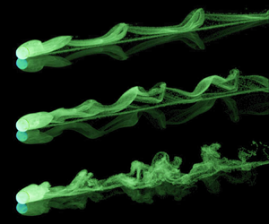
The experimental observation of the mirror-symmetric wake mode identified in the numerical simulations proved to be extremely difficult, or even impossible. The experimental counterparts of the numerical wake structures in figures 11–13 are shown in figure 15. At the lowest Reynolds number, $Re^*=136$, unlike the behaviour observed in the numerical simulations, the wake is always found to be asymmetric with respect to the centre plane, and the sphere always exhibited irregular motion in the lateral direction. A likely explanation involves imperfections of the experimental configuration, such as irregularities of the sphere geometry or a non-perfect flatness of the Plexiglas plate, and in particular the presence of dust particles on the slope surface. With the extremely small forces driving the sphere motion at low $Re^*$, encountering the tiniest speck of dust may deviate the sphere trajectory temporarily sideways, before the pull of gravity redirects it again down the slope. As discussed above, the numerical simulations show that cross-slope oscillations are almost neutrally stable at this Reynolds number, so this behaviour is not all that surprising. The large-scale shape of the dyed sphere wake in figure 15(a) may simply be the result of the imperfection-induced sphere motion. However, it is also possible that the onset of sphere oscillations occurs at lower Reynolds numbers for smaller gaps, noting that the drag and side force coefficients are indeed strongly gap-dependent.

Figure 15.

Experimental dye visualisations of the wake of freely rolling spheres for (a) $Re^*=136$, (b) $Re^*=153$ and (c) $Re^*=241$. Views from above, $\beta =2.2$ in all cases.

At higher Reynolds numbers, the match between the experimental and numerical simulations is much better. The experimental dye (figure 15) and numerical tracer (figure 13) visualisations for $Re^*=153$ and 241 show similar wake structures, structure sizes, sideways motion, wavelengths and complexity. Relative to the uniform rolling case, the onset of cross-slope motion and loss of periodicity occur at considerably lower Reynolds numbers. The shedding of vortex loops persists up to higher $Re^*$, as seen in the dye visualisation example of figure 16.

Figure 16.

(a) Oblique side view of an experimental dye visualisation of vortex loops in the rolling sphere wake at $Re^*=412$ and $\beta =2.2$. (b) Similar views of passive tracer visualisations from simulations for $\beta =2.2$. Top to bottom: $Re=136$, 153 and 412. Note that the reflection from the plane surface has also been mimicked in these images. Animations of these visualisations are also available as supplementary movies 1–4, available at https://doi.org/10.1017/jfm.2023.250.

4.4. Unsteady forces and sphere vibrations

In this subsection, the time-dependent force coefficients and fluid velocities predicted by the numerical simulations are presented for various Reynolds numbers ($100\le Re^*\le 200$) and density ratios ($0.8\le \beta \le 10$), again for the single gap ratio $G/d=0.005$. The effect of the gap size is addressed in the next subsection.

Figure 17 shows the numerically determined time evolution of the drag, lift and side force coefficients, and of the downslope and lateral velocity component of the sphere, which is initially at rest. In these plots, the velocity scale used to non-dimensionalise the force coefficients is the instantaneous speed, i.e. $\sqrt {(v^*)^2 + (u^*)^2}$, noting that substantial cross-slope velocities are induced for higher Reynolds number and low mass ratios. The asymptotic state can take some time to be reached, depending on the Reynolds number and mass ratio. For $Re^*=100$ and $\beta =0.8$, the final asymptotic state has not been reached even after $t^*=300$, which corresponds to a downslope distance of approximately $300d$ from the initial position! The initial transient is shorter for the lighter, less inert spheres, as expected, similar to case of the freely rolling circular cylinder (Houdroge et al. Reference Houdroge, Leweke, Hourigan and Thompson2020).

Figure 17.

Time evolution (from rest) of the force coefficients and sphere velocity components for different Reynolds numbers and density ratios.

At $Re^*=100$, except for the lowest mass ratio case, the force coefficients reach a constant value as the flow attains a steady state. For $\beta =0.8$, as discussed, the fluid–structure system is unstable to cross-slope oscillations. Hence the onset of cross-slope oscillations depends on the mass ratio of the sphere with positively buoyant spheres developing such oscillations prior to the downslope unsteady transition. At $Re=150$, above the transition to unsteady downslope flow, the asymptotic state is strongly dependent on mass ratio. For $\beta =10$, the final state appears to be quasi-periodic but without cross-slope oscillations. Decreasing the mass ratio to $\beta =3$ results in the development of cross-slope oscillations and an increasingly chaotic asymptotic flow state. For the positively buoyant case $\beta =0.8$, the wake does not even transition through a near-periodic symmetrical shedding state with large cross-slope oscillations developing rapidly. The final state is very irregular with maximum cross-slope velocities almost 50 % of the downslope component. Because of this, the final average downslope velocity is well below that seen in the two heavier sphere cases. Strongly irregular fluctuations and lateral forces are observed for all density ratios at $Re^*=200$.

It may be noted that when irregular lateral forces appear, the running mean of the corresponding coefficient $C_{D,y}$ is not zero, which can result in a sideways drift of the sphere (see below).

The two components of the sphere velocity are presented in figures 17(m–o). As expected, the cross-slope velocity $v_s^*$ is zero when the flow is steady ($Re^*=100$) and plane-symmetric ($Re^*=150$ and $\beta =10$), since the sphere rolls in a straight line down the slope in these cases. In the more irregular asymmetric states at $Re^*=200$ (and for $\beta =0.8, 3$ at $Re^*=150$), the lateral sphere velocity oscillates around zero, most of the time with a small non-zero mean. The evolution of the $x$-velocity down the slope depends on both $Re^*$ (asymptotic mean value) and $\beta$ (i.e. the duration of start-up transient and the amplitude of the oscillations in the unsteady states).

Figure 18 shows the position of the sphere along and across the slope as function of time, and figure 19 gives the approximately adjusted coordinates, representing the deviations from the mean trajectory. The sphere rolls in a straight line at constant speed when the flow is steady, and exhibits vortex-induced vibrations when the flow is unsteady. Even close to the transition at $Re^*=150$, the oscillations are irregular. As $Re^*$ is increased to 200, the flow becomes more chaotic. Particularly noticeable for $\beta =3$ at both $Re^*=150$ and $200$, the frequency of the lateral vibration is only about half that of the inline oscillation (see also figure 23). Such a low frequency is also present in the evolution of the lateral force coefficient for a uniform rolling sphere, in the regime just above the onset of asymmetric wake flow (Rao et al. Reference Rao, Passaggia, Bolnot, Thompson, Leweke and Hourigan2012).

Figure 18.

Position of the sphere (a–c) along and (d–f) across the slope, from the numerical simulations.

Figure 19.

Fluctuating position of the sphere (a–c) along and (d–f) across the slope, obtained by subtracting the values of the mean trajectory. The time interval shown represents the asymptotic state after the initial transient.

The time traces of the adjusted sphere position can be used to obtain the oscillation amplitude of the sphere in the unsteady regime, although well above the transition to unsteady flow, the amplitude variation becomes chaotic. Figure 20 shows that the inline vibration amplitude ($A_x^*$) increases with the Reynolds number $Re^*$ and decreases with the density ratio $\beta$.

Figure 20.

Amplitude of oscillation, scaled by the sphere diameter in the direction of the slope. Symbols correspond to different density ratios, as before.

So far, only results from the numerical simulations at constant gap size between the sphere and the wall have been shown. In the experiments, it is likely that an effective gap (of unknown size) existed, due to the surface roughness of the sphere and/or wall and the presence of impurities. Keeping this in mind, it is nevertheless possible to make a few comparisons between numerical and experimental results concerning the flow-induced sphere vibrations. The next subsection will take a closer look at the influence of gap size and roughness on the effective drag forces, which can be deduced from the observed sphere velocity.

For the comparison with the simulations, an experimental case at moderately high Reynolds number ($Re^*=241$) is chosen, for which the effect of impurities such as dust particles generating spurious lateral sphere motions are expected to be weak (see § 4.3, figure 15). Figure 21 illustrates how the trajectory of the sphere rolling down the transparent inclined plate in the water tank is determined, by tracking the sphere in the corresponding video sequence. From this, the absolute and adjusted inline and lateral positions of the sphere as functions of time are calculated. The results in figures 22(c,d), which have been filtered to reduce high-frequency noise, are very similar to the numerical predictions for the same case shown in figures 22(e,f). The non-dimensional mean velocity of the sphere, given by the slope in figure 22(a), is approximately 25 % lower than in the simulations. According to (2.17) and (2.18), this implies a higher effective drag coefficient, which is likely to be related to the effective gap size. Despite this difference, the amplitudes and frequencies of the inline and lateral sphere vibrations in figures 22(c,d) are very similar to the numerically predicted ones, suggesting that these frequencies are dependent on the outer flow and not on the gap flow.

Figure 21.

Experimental trajectory of the sphere as it rolls through the field of view (from left to right). The image is stretched in the vertical direction by a factor 10, in order to emphasise the lateral sphere motion. Here, $Re^*=241$ and $\beta =2.2$.

Figure 22.

Sphere coordinates obtained from the visualisation illustrated in figure 21 for $Re^*=241$ ($\overline {Re}=270$) and $\beta =2.2$: (a,b) non-dimensional positions along and across the slope; (c,d) adjusted positions (deviations from the mean trajectory); (e,f) similar adjusted positions from the numerical simulation at the same Reynolds number.

Figure 23 shows a collection of numerically and experimentally determined frequencies of the sphere vibrations for a moderately buoyant case. The frequencies ($\,f$) are expressed in the form of a non-dimensional Strouhal number, defined as $St=fd/\bar {u}_s$. They are given as function of the Reynolds number $\overline {Re}$ based on $\bar {u}_s$, in order to allow a comparison with the results for a uniform rolling sphere. The vibration frequencies of the freely rolling sphere are very close to the wake frequencies for uniform rolling, for both the inline motion and the lateral displacement.

Figure 23.

Strouhal numbers of the sphere motion compared to the wake frequencies of the uniform rolling sphere (Rao et al. Reference Rao, Passaggia, Bolnot, Thompson, Leweke and Hourigan2012). The upper and lower branches correspond to fluctuations in the inline and lateral directions, respectively.

4.5. Effects of roughness and gap size

When comparing the predictions from numerical simulation and experimental measurements of a freely rolling sphere driven by gravity, a significant discrepancy was found concerning the non-dimensional asymptotic rolling velocity (figure 5). Since this velocity is determined mainly by the drag coefficient (2.17), which in turn depends on the size of the gap between the sphere and the surface (see figure 24), it is reasonable to assume that part of the observed difference between the results may be due to a difference in the effective gap size. Whereas this size was fixed and constant in the simulations, it was uncontrolled and unknown in the experiments. As mentioned in the Introduction, surface roughness had been considered in the past as a possible source for causing an effective gap between the two solids. However, this idea was discarded by Goldman et al. (Reference Goldman, Cox and Brenner1967), and more recently again by Wardhaugh & Williams (Reference Wardhaugh and Williams2014), since various experimental studies on freely rolling spheres did not show evidence of a dependency of the drag on roughness.

Figure 24.

Predicted evolution of the mean effective drag coefficient with the gap ratio at two Reynolds numbers, for a uniform rolling sphere.

Figure 25 shows a collection of experimental results concerning the effective drag coefficient $\bar {C}'_D$ (see (2.18)) of a sphere rolling down an incline under gravity, including the present measurements, which are in good agreement with previous work. They are presented as functions of the Reynolds number $\overline {Re}$, based on the mean velocity, in the usual log–log scaling. This representation, in combination with the relatively large scatter, in particular in the intermediate Reynolds number range, hardly allows the identification of small differences associated with variations in the surface roughness.

Figure 25.

Mean effective drag coefficient as a function of Reynolds number, determined in various experimental studies. The present results cover the range $15<\overline {Re}<900$.

In the present study, we have carried out a series of measurements with spheres made of the same material rolling down the same inclined surface, where the asymptotic rolling velocities were determined with high accuracy. The difference between the spheres was their diameter and therefore, assuming a similar surface structure, their relative roughness. The results from these experiments are shown in figure 26.

Figure 26.

Close-up of the $\overline {Re}$–$\bar {C}'_D$ relation for spheres of the same material (acrylic), but of different diameters, compared to the values obtained from numerical simulations using different gap ratios.

A discussion is now presented to address the observed discrepancy between the results of the direct numerical simulations and the experiments. At the gap ratio $G/d=0.005$ imposed throughout the numerical study, the computed drag coefficient was significantly lower than the drag calculated from the experimental runs at equivalent Reynolds numbers, as shown in figure 26, which focuses on the experiments with the acrylic spheres in the range $15\le \overline {Re}\le 250$ and the numerical predictions for $30\le \overline {Re}\le 125$ and $0.0002\le G/d\le 0.01$. Additionally, figure 24 gives the detailed variation of the computed $\bar {C}_D'$ versus the gap ratio for $\overline {Re}=50$ and 100. It is clear from these figures that the effective drag is particularly sensitive to the imposed gap and tends to increase as the latter decreases. Extrapolating the curves of figure 24 towards an equivalent gap at which the computed drag coefficient matches the experiments, we find that the numerical simulations would have to be carried out with a gap ratio of the order of $10^{-4}$–$10^{-5}$, suggesting an effective gap (and equivalent surface roughness) of order $10^{-6}$–$10^{-7}$ m. This would require an increased resolution in the gap region and a reduced time step, thus very large computational costs, beyond the scope of the present study. It is important to note that while the drag is sensitive to the imposed gap, the large-scale flow field remains practically independent of it (see Stewart et al. Reference Stewart, Thompson, Leweke and Hourigan2010a).

Another significant observation from figure 26 is that the drag coefficients of the acrylic spheres of different diameters follow the same trend, but are translated upwards in the direction of the $y$-axis as the diameter is increased. This trend is consistent with each sphere having a similar absolute surface roughness, leading to a smaller effective gap ratio for larger spheres.

As described in the Introduction, the problem of a sphere moving along a wall at a fixed height was solved by Goldman et al. (Reference Goldman, Cox and Brenner1967) and O'Neill & Stewartson (Reference O'Neill and Stewartson1967) using the Stokes approximation. When there is contact between the particle and the wall, their solutions suggest that the fluid exerts an infinite resistance force opposing the movement of the sphere, thus inhibiting its motion. In addition, the lift force is predicted to be zero, while as the sphere is moved closer to the wall, the rotational to translational velocity approaches $1/4$. The idealised mathematical model used to describe this flow problem is therefore insufficient to provide a complete understanding of the physics behind the rolling of the sphere.

Since those studies, others have extended the theoretical analysis to consider finite Reynolds number effects (Krishnan & Leighton Reference Krishnan and Leighton1995; Cherukat & McLaughlin Reference Cherukat and McLaughlin1994; Zeng et al. Reference Zeng, Najjar, Balachandar and Fischer2009; Lee & Balachandar Reference Lee and Balachandar2010) and the likely effect of surface roughness (Krishnan & Leighton Reference Krishnan and Leighton1995; Prokunin Reference Prokunin2003). These further studies still indicate that the drag force remains infinite for surfaces in contact; however, the effect of surface roughness is to maintain an effective gap between the surfaces, while the interaction between surface roughness elements can provide a retarding frictional force to enable effective rolling without slip (Krishnan & Leighton Reference Krishnan and Leighton1995), which is observed in practice, at least for small slope angles (Wardhaugh & Williams Reference Wardhaugh and Williams2014). Thus although Goldman et al. (Reference Goldman, Cox and Brenner1967) noted that the Carty (Reference Carty1957) data lie on a single curve for $\overline {Re}<60$ and therefore eliminated the effect of surface roughness, the present investigation shows that the data can actually follow different curves within this range. This can be attributed to the fact that the current experiments resulted in more data points and a more detailed examination of the outcome than in Carty (Reference Carty1957).

The Stokes flow analysis of Goldman et al. (Reference Goldman, Cox and Brenner1967) provides a prediction of the drag on a rolling sphere in the limit of zero Reynolds number. The solution can be constructed from the combination of expansions for translational and rotational motion. Assuming that the sphere rolls so that the rotational and translational speeds are the same, which is the case here, the effective drag is predicted to be

(4.6)\begin{equation} \bar{C}_{D0}' = \frac{1}{\overline{Re}} \left[-44.2 \log_{10} (G/d) + 34.0 \right], \end{equation}

again combining the drag and torque contributions as in (2.18). This is obtained directly from expressions for the drag and viscous torque provided in Goldman et al. (Reference Goldman, Cox and Brenner1967), with the coefficients evaluated explicitly for the more convenient $\log _{10}$ based expression given here. For small gaps, one could expect that the total effective drag can be expressed as the sum of a gap drag, given by the above expression, and what one might call the wake drag, $\bar {C}'_{D,wake}$, i.e.

(4.7)\begin{equation} \bar{C}_D' \approx \bar{C}_{D0}' (\overline{Re},G/d) + \bar{C}_{D,wake}' (\overline{Re}). \end{equation}

Here, it is assumed that the wake drag varies with Reynolds number, but has little dependence on the gap ratio for small gaps. Figure 27 shows the wake drag variation for $G/d=0.005$ and Reynolds numbers up to 300. Also shown in this figure are values calculated from the numerical data shown in figure 26, covering gap ratios $0.0002 \leq G/d \leq 0.01$, showing a good collapse of the results according to the assumed variation given by (4.7). For $1 \leq \overline {Re} \leq 300$, $\bar {C}_{D,wake}'$ varies only over the relatively modest range 1–1.5, with an approximate quadratic fit for $\overline {Re} > 5$ given by

(4.8)\begin{equation} \bar{C}'_{D,wake} = 1.70 - 0.136 (\log_{10}\overline{Re}) - 0.0716 (\log_{10}\overline{Re})^2, \end{equation}

as shown by the solid line in figure 27.

Figure 27.

Predicted wake drag ($C_{D,wake}'$) as a function of Reynolds number (square symbols) for $G/D=0.005$. Overlaid are wake drag predictions (blue circles) using all the numerical data from figure 26, covering gap ratios $0.0002 \leq G/d \leq 0.01$. An approximate quadratic fit over $5 \leq \overline {Re} \leq 300$ is shown by the solid curve.

Note that the wake drag should approach zero as the Reynolds number and gap approach zero, given that the simulated flow (drag force) should approach the Goldman solution given by (4.6). It is expected that this behaviour would be seen at small Reynolds numbers ($Re \lesssim O(1)$) as the gap size is reduced further so that the Goldman approximation becomes more accurate. In any case, for $Re \leq 1$ and $G/d=0.005$, the wake drag contribution is order 1 % or less than the overall drag. It is only at significantly higher Reynolds numbers that it becomes an important contribution. By $\overline {Re}=100$, there is approximately an even split between the gap and wake drag components.

For $\overline {Re}=100$, figure 26 shows that the maximum effective drag from experiments occurs for the largest sphere ($d=7.9$ mm). Using (4.7) to estimate the corresponding effective gap gives an estimate $G \approx 2 \times 10^{-8}$ m. While indeed very small, this is not necessarily beyond the bounds of expected surface roughness for polished acrylic surfaces (see e.g. Al Rifaiy Reference Al Rifaiy2010).