1. The Physical Church-Turing Thesis

Physicists often interpret the Church-Turing Thesis as saying something about the scope and limitations of physical computing machines. Although this was not the intention of Church or Turing, the Physical Church Turing thesis is interesting in its own right. Consider, for example, Wolfram's formulation:

Wolfram's thesis consists of two parts: (a) Any physical system can be simulated (to any degree of approximation) by a universal Turing machine (b) Complexity bounds on Turing machine simulations have physical significance. For example, suppose that the computation of the minimum energy of some system of n particles takes at least exponentially (in n) many steps. Then the relaxation time of the actual physical system to its minimum energy state will also take exponential time.

An even more extreme formulation of (more or less) the same thesis is due to Aharonov (Reference Aharonov1998): A probabilistic Turing machine can simulate any reasonable physical device in polynomial cost. She calls this The Modern Church Thesis. Aharonov refers here to probabilistic Turing machines that use random numbers in addition to the usual deterministic table of steps. It seems that such machines are capable to perform certain tasks faster than fully deterministic machines. The most famous randomized algorithm of that kind concerns the decision whether a given natural number is prime. A probabilistic algorithm that decides primality in a number of steps which is polynomial in the size of the input, and with a high probability of success existsFootnote ¹. No deterministic algorithm to decide primality in polynomial number of steps is known to exist. This is an open problem, as is the general question whether polynomial time probabilistic Turing machines are really faster than deterministic ones.

Apart from this modification Aharonov's formulation is identical to that of Wolfram. There are many other formulations of a “physical Church-Turing thesis” in the literatureFootnote ². In fairness one should add that Wolfram was fully aware that quantum mechanics may falsify his thesis. Aharonov, writing in the late nineties, formulated the thesis in order to show its incompatibility with quantum theory.

Quite independently of quantum mechanics, however, part (a) of Wolfram's thesis is false. Pour-El and Richards (Reference Pour-El and Richards1981) proved that some classical physical systems cannot be simulated by any Turing machine. Their example is a three dimensional wave with strange, but nevertheless recursive initial conditions. The example is contrived but it may indicate a more widespread phenomenon. Perhaps this is the reason why Aharonov refers to “ reasonable physical device” in her formulation. Here we shall concentrate on part (b) of the thesis and deal only with physical systems that can be simulated by a computer. We shall be concerned primarily with the computation cost of the simulation.

Before we get to our main concern let me note that there really is no relation between the physical and the original Church-Turing thesis (see Shagrir and Pitowsky Reference Shagrir and Pitowsky2002 for more details). Turing was interested in the decision problem for formal systems, that of arithmetic in particular. This means that he was concerned with a concept of computation that is tightly related to the concept of proof. Now, the concept of proof by its very nature entails that proofs could be validated, at least in principle, by checking each step for correctness. It follows that the concept of computation that is relevant for logic should also have that character, it should be an idealization of (symbolic) computation with a pencil and paper. Indeed, every step that a Turing machine takes can be identified and checked. The Church-Turing thesis is simply the assertion that the language of Turing machines (or any other universal programming language) is the correct idealization for that purpose. Turing (Reference Turing1936) provided a very powerful argument to that effect.

However, it does not analytically follow from the concept of computation that all computations should be amenable to tests of validity. For example, there is a long historical tradition of analogue computations, which use continuous physical processes. One can check such a computation by running the device again, or by verifying the physical theory of the device by other means. Obviously, these procedures do not constitute a test of validity. Turing, who was also involved in the design of analogue computers, did not refer to them, or any other physical device, in his thesis.

2. Physical and Computational Parameters

In order for the physical Church-Turing thesis to make sense we have to relate the space and time parameters of physics to their computational counterparts: memory capacity and number of computation steps, respectively. There are various ways to do that, leading to different formulations of the thesis (Pitowsky, Reference Pitowsky1990). For example, one can encode the set of instructions of a universal Turing machine and the state of its infinite tape in the binary development of the position coordinates of a single particle. Consequently, one can physically ‘realize’ a universal Turing machine as a billiard with hyperbolic mirrors (Moore Reference Moore1990; Pitowsky Reference Pitowsky1994).

However, the most intuitive connection between abstract Turing machines and physical devices appear in the pioneering work of Gandy.Footnote ³ A discrete deterministic mechanical device is a physical system such that:

1. 1. It consists of a (potential) infinity of atomic parts.

2. 2. There are only finitely many kinds of atomic parts.

3. 3. “There is a lower bound on the… dimension of every atomic part.”

4. 4. “There is an upper bound on the speed of propagation of change,” so that only local interactions between the parts are possible.

5. 5. At each stage of its dynamics only finitely many parts change their state.

Such a system is characterized by its set of states and a function F, from the set of states to itself, which represents the dynamics. It begins in some initial state S ₀, then it is transformed to the state F(S ₀), after another iteraction it is transformed to the state F(F(S ₀)) and so on. The time parameter is taken to be discrete and the dynamics F is constrained by principles 1–5. Not surprisingly, perhaps, Gandy proved that devices of this kind can be simulated by Turing machines.

To make things more concrete, assume that the device under consideration is one dimensional and is made of three types of atoms, denoted by ▪, ♠, and ▴. Assume, for simplicity, that each atom can be in one of two intrinsic states + or −, so that the atom ♠ in the + state is denoted by ♠⁺ and so on. The state of the ‘device’ is then completely characterized by the intrinsic state of each atom and the order in which the atoms appear in the one dimensional array. Since the dynamics is constrained by principles 1–5, the most it could do at each stage is to induce a finite permutation of the atoms, and change the intrinsic state of a finite number of atoms. Suppose that the initial state of the system is

then the dynamics F may transform the system in the following way

Another initial state S′₀ will be transformed differently, for example

The central principle of quantum mechanics is the principle of superposition. If S ₀ and S′₀ are two possible quantum states of the system, so is any of their superpositions. Thus, if we want to extend Gandy's conceptions we should include states of the device like that is,

which is transformed by F to,

In the quantum context the dynamics F (which is represented as a unitary operator) may add phase factors like $e^{i\alpha _{1}}$ to each component. This is a crucial difference which will play an important role in the sequel.

Can we simulate such dynamics on a Turing machine? The answer is yes! (Deutsch Reference Deutsch1985). If the system starts from a finite superposition of states, we can calculate the dynamics of each element of the superposition separately on one Turing machine, and then add the results with the proper (rational approximation) of the phase. If the superposition is infinite we can approximate it by a finite one to any degree of accuracy. The point is, however, that it seems impossible to simulate the quantum system in real time or even at polynomial cost. If the number of superimposed states is very large then simulating the dynamics of each one of them separately on a serial machine takes a long time. The real dynamics in our quantum world runs “in parallel”. This is the source of the quantum speed-up.

3. Quantum Parallelism

But things are not so simple. Consider, for example, the SATISFIABILITY problem: You are given as input a proposition in the propositional calculus and you have to decide if it has a satisfying truth assignment. There is an obvious algorithm to solve the problem: Try the truth assignments one by one, using the truth tables. If you run into a satisfying truth assignment you stop on YES. Otherwise you print NO. The trouble is that a proposition with n atoms has 2ⁿ possible truth assignments. Thus, in the worst case, the number of steps the algorithm takes is exponential in the size of the input. The bigger trouble is that no (essentially) better algorithm is known to exist. This is the most important open problem in theoretical computer science (Gary and Johnson Reference Gary and Johnson1979).

It seems superficially that quantum parallelism suits this problem. We can easily represent the proposition and the truth assignments by the states of a quantum system. We first encode them as a sequence of zeroes and ones, as is done in a conventional computer. Then we associate with each 0 a particle in the state |0〉 = |+〉 = “spin up in the z-direction” and with each 1 a particle in the state |1〉 = |−〉 = “spin down in the z-direction”. Then, with each truth assignment (on n atoms) there corresponds a state of n particles |∊₁〉 |∊₂〉 … |∊ _n〉, where ∊ _i ∊ {0, 1}. Similarly, we can encode the proposition in terms of some sequence, denote it by | … Φ … 〉. Its length equals the number of bits it takes to encode the proposition on a conventional Turing machine. We also have to keep a particle whose state encodes the result | YES〉 or | NO〉. We begin with the state | … Φ … 〉 |∊₁〉 |∊₂〉 … |∊ _n〉| NO〉. The conventional program that uses truth tables to check the truth value of a given proposition Φ, given an assignment ∊₁, ∊₂, … , ∊ _n, can be represented as a unitary transformation on the set of states.Footnote ⁴ Our initial state is then transformed to | … Φ … 〉|∊₁〉 |∊₂〉 … |∊ _n〉| T(Φ, ∊₁, ∊₂, … , ∊ _n,) 〉 where T(Φ, ∊₁, ∊₂, … , ∊ _n) = YES if ∊₁, ∊₂, … , ∊ _n satisfies Φ and = NO otherwise. But instead of checking the assignments one by one we can start with the initial state

Then we rotate each one of the spins corresponding to the truth assignment to the + x direction. This takes n simple unitary transformations, each on a 2-dimensional space. Since 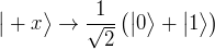$\big\vert +x\big\rangle \rightarrow \frac{1}{\sqrt{2}}\left(\big\vert 0\big\rangle +\big\vert 1\big\rangle \right)$ the result is therefore

Only now we apply the unitary transformation associated with the satisfiability test. We obtain

Testing a single truth assignment takes a small number of steps (a fixed polynomial in n). Here we have tested all the 2ⁿ assignments “at once”. Unfortunately this quantum miracle helps us very little in solving SATISFIABILITY. In a sense the state (3) encodes the solution, but we cannot retrieve it in polynomial time. If we perform a measurement to check the state of the particle in the “result box” (i.e. the particle that encodes the result | YES〉 or | NO〉) the state (3) collapses. If there is only one satisfying truth assignment the probability of finding it is then 2⁻ⁿ. This is just the probability of guessing the satisfying truth value at the outset. A probabilistic Turing machine can be programed to guess assignments and check them. It will perform equally well and we have thus gained nothing.

In order to use the principles of quantum mechanics to enhance computations we have to create “clever” superpositions that increase the probability of success considerably above that of a pure guess. But to create a superposition also takes time. Usually exotic superpositions of n particle states are not stable in nature. In the above example we begin from a product state (1) and by n local operations create (2) which, incidently, is also a product state. In general, a quantum computation begins with a product state and the creation of the superposition is part of the (quantum) program. At each stage such a program performs a unitary operation on at most two particles at once.Footnote ⁵ Such an operation is called a step. It turns out that in this way we can approximate any superposition to any degree of accuracy (Deutsch Reference Deutsch1985). However, the number of steps required is usually exponential (in the number of particles).

In order to see what we could do with clever superpositions (if we could create them fast) consider the problem called GRAPH ISOMORPHISM. Again, nobody knows how to solve it in polynomial time, although it is believed to be somewhat simpler than SATISFIABILITY (Gary and Johnson Reference Gary and Johnson1979). A (simple) graph is a pair G = (V, E) where V is the set of vertices, which we can take to be an initial segment of the set of natural numbers V = {1, 2, … , n}, and E the set of edges is a subset of the set of pairs E ⊆ {{ i, j}; 1 ≤ i < j ≤ n}. Two graphs G = (V, E) and G′ = (V, E′), with the same set of vertices V, are called isomorphic if there is a permutation π of the set of vertices V = {1, 2, … , n} such that { i, j} ∊ E if and only if {π i, π j} ∊ E′. The computation task in GRAPH ISOMORPHISM is to decide if two given graphs are isomorphic.

To represent a graph G = (V, E) by a quantum state we can use $\frac{1}{2}$ n(n − 1) particles and label them by the pairs { i, j} with 1 ≤ i < j ≤ n. Now, define χ(i, j) = 1 when { i, j} ∊ E and = 0 otherwise, and denote

Then the graph G is uniquely characterized by the state | G〉. Similarly, define the state | G′〉 corresponding to the graph G′ and its function χ′(i, j) which equals 1 when { i, j} ∊ E′ and 0 otherwise. Now define the superposition

and a similar superposition | SG′〉 for the graph G′. The sum in (5) ranges over all permutations π of {1, 2, . . . , n}. It is easy to see that if G is isomorphic to G′ then | SG′〉 = | SG〉. Moreover, in case G and G′ are not isomorphic | SG〉 is orthogonal to | SG′〉, that is 〈 SG | SG′〉 = 0. If we could create the superposition (5) in a number of steps that is polynomial in n then we would have made an important step toward the solution of GRAPH ISOMORPHISM in polynomial time. However, nobody knows how to do that.

4. Shor's Algorithm

So far the most dramatic example of a possible quantum speed-up concerns the problem of FACTORING, the determination of the prime divisors of a given natural number. Recall that the binary representation of a natural number n takes ~log₂ n bits. We have already noted that to decide whether n is prime takes a number of steps which is a polynomial in log₂n, using a probabilistic Turing machine. Nobody knows how to factor numbers in polynomial time, not even on a probabilistic Turing machine. This is yet another open problem in the theory of computational complexity. Modern cryptography and Internet security are based on these two facts: it is easy to find large prime numbers fast, and it is hard to factor large composite numbers in any reasonable amount of time. Many protocols such as public key and electronic signature are based on these facts (Giblin Reference Giblin1993). Therefore, the discovery that quantum computers can solve FACTORING in polynomial time has had a dramatic effect.Footnote ⁶ The implementation of the algorithm on a physical machine will have an economic, as well as scientific consequences. Unfortunately, the engineering of real quantum computers faces many obstacles which we shall not discuss here (see Ekert and Jozsa Reference Ekert and Jozsa1996, Aharonov Reference Aharonov1998).

Let L be a natural number. Any natural number a such that 0 ≤ a ≤ 2^L−1 has a binary representation $a=\sum_{k=0}^{L-1}a_{k}2^{k}$ where a ₀, a ₁, . . . , a _L−1 ∊ {0, 1}. We shall represent the number a by the state | a〉 = | a _L−1〉 | a _L−2〉 … | a ₀〉. The Discrete Fourier Transform (modulo 2^L) is the map that takes each number state | a〉, 0 ≤ a ≤ 2^L−1 to the superposition of 2^L states

The key to Shor's algorithm is the following theorem: If we can construct DFT _L (a) from | a〉 in a number of steps which is polynomial in L then we can factor any given number n in a number of steps which is polynomial in log₂n. This is the central mathematical observation in Shor's paper and it has little to do with quantum mechanics. So the trick, really, is to create the superposition DFT _L(a) fast, and the rest is an ingenious number theoretic argument which we shall skip.Footnote ⁷ Note that apart from the phase factors exp $\left(\frac{2\pi iac}{2^{L}}\right)$ the state (6) is similar to (2). Both are sums, with equal weights, over all possible 0, 1 states of a given length. The phase factors make all the difference.

To create DFT_L(a) from | a〉 we shall use two types of elementary unitary operations. The first is just a $\frac{\pi }{2}$ rotation performed on the spin of a single particle. It is given by the matrix

So that by the operation of A we have $\big\vert 0\big\rangle \rightarrow \frac{1}{\sqrt{2}}\left(\big\vert 0\big\rangle +\big\vert 1\big\rangle \right)$ and $\big\vert 1\big\rangle \rightarrow \frac{1}{\sqrt{2}}\left(\big\vert 0\big\rangle -\big\vert 1\big\rangle \right).$ The second type of unitary map operates on the state of two particles and is given by the diagonal matrix

So that |0〉 |0〉 → |0〉 |0〉, |0〉 |1〉 → |0〉 |1〉, |1〉 |0〉 → |1〉 |0〉, and finally |1〉 |1〉 → e ^iθk |1〉 |1〉. We can imagine the physical realization of these operations as gates, where the particle, or pair of particles, enter it from the left and emerge from the right in the transformed form. Denote by A _i the operator A acting on the state of particle i, i = 0, 1, … , L − 1. For i, j with 0 ≤ i < j ≤ L − 1 denote by B _{i j} the operator B _(j−i) acting on particles i, j. The creation of DFT _L (a), in the case L = 5, is given by the following sequence of operators

And the general case follows the same pattern. The total number of operators (or gates) is $\frac{1}{2}$ L(L + 1), which is a polynomial in L.

It seems, therefore, that the physical Church-Turing thesis is false. Turing provided us with an excellent conceptual tool for the analysis of the theoretical properties of algorithms, but it seems to be the wrong tool for the analysis of physical processes. It is very likely that quantum automata can “shortcut a computationally irreducible process”. Other physical phenomena, such as space-time singularities, may have even more dramatic theoretical consequences for the scope and speed of computations.Footnote ⁸