Implications
To decrease mastitis frequency, it is necessary to have adequate measures of the biological mechanisms underlying the disease. Here, we applied a simple linear state-space model on monthly milk somatic cell scores collected routinely in dairy databases. We show the model is highly accurate, very flexible and relatively easy to implement. It allows the identification of disease sub-phenotypes corrected for measurement errors and accounts for the dynamics of the response to the infection. As such, it may shorten the gap between genotype and phenotype expression and help design personalized treatment.
Introduction
Bovine mastitis is a frequently occurring disease with great economic consequences. To find tools that will decrease its frequency, it is necessary to have adequate measures of the biological mechanisms underlying the disease, which is not easy to obtain in field conditions. Here, we propose to combine clinical and subclinical information (obtained in a field study) in a state-space model to obtain measures representative of the defence mechanisms used by the mammary gland to fight infection.
Information on clinical cases is valuable because cows that experienced a case previously have a greater probability of developing a subsequent one (Steeneveld et al., Reference Steeneveld, Hogeveen, Barkema, van den Broek and Huirne2008). In addition, records on clinical cases provide continuous information not limited to recording at fixed intervals. However, in practice, data collection on clinical cases depends heavily on the willingness of the observers to collect and report the information so that data may be sparse and subjective.
Information on subclinical cases is also important because defence mechanisms operate before the apparition of clinical signs. To detect subclinical mastitis, owners of automatic milking systems have access to in-line milk-sensing measures such as milk electrical conductivity, yield or temperature, but the frequent occurrence of false-positive alerts has thwarted their widespread use (Hovinen and Pyorala, Reference Hovinen and Pyorala2011). Researchers have also looked for biomarkers such as milk lactoferrin, haptoglobin or NGase (Soyeurt et al., Reference Soyeurt, Bastin, Colinet, Arnould, Berry, Wall, Dehareng, Nguyen, Dardenne, Schefers, Vandenplas, Weigel, Coffey, Theron, Detilleux, Reding, Gengler and McParland2012), but their measurements are often costly on a routine basis. The most frequent method used to detect subclinical mastitis is based on the measurement of patterns of monthly milk somatic cell counts (SCC). Indeed, SCCs are typically elevated in the presence of intramammary infection and are commonly recorded at (usually) monthly milk recording visits. Many models have been proposed to analyze SCC patterns. Some are based on logistic regression (Kristula et al., Reference Kristula, Curtis, Galligan and Bartholomew1992) or alternative traits (de Haas et al., Reference De Haas, Veerkamp, Barkema, Grohn and Schukken2004). Others draw on mixture (Detilleux and Leroy, Reference Detilleux and Leroy2000; Jamrozik and Schaeffer Reference Jamrozik and Schaeffer2010) and hidden Markov models (Detilleux, Reference Detilleux2011; Robertson et al., Reference Robertson, Sawford, Gunawardana, Nelson, Nathoo and Stephen2011). Advantages of mixture and hidden Markov models include their flexibility associated with their ability to represent observed and hidden states, and their capacity to cope with missing observations. However, they are limited by the finite number of possible hidden states (e.g. infected or not).
State-space models are based, like hidden Markov models, on the assumption that an unobserved variable explains the observed variation and evolves with Markovian dynamics. The main difference is that hidden Markov models use a discrete hidden state variable with arbitrary dynamics, whereas state-space models use a continuous state variable with parametric forms for the transition dynamics (Roweis and Ghahramani, Reference Roweis and Ghahramani1999). In the context of bovine mastitis, hidden variables may represent defence mechanisms against mastitis pathogens that cannot be observed accurately under field conditions. For example, SCCs are a mix of leukocytes and epithelial cells (Bradley and Green, Reference Bradley and Green2005). Of both cell types, leukocytes serve as a major defense mechanism to fight disease infection (even if the role of epithelial cells should not be disregarded). If hidden variables are more accurate as indicators of cell dynamics during infection, they will be useful in the search for personalized treatment or for genes and gene pathways that are altered in response to the presence of pathogenic bacteria (Pighetti and Elliott, Reference Pighetti and Elliott2011).
State-space models are also particularly well suited for Bayesian model-fitting approaches and this permits a great degree of flexibility including, for example, nonlinear, non-Gaussian or multivariate processes. Moreover, time steps do not have to correspond to a fixed unit of real time or to follow equally spaced time intervals.
Therefore, the goal of this paper is to validate the use of a linear state-space model (LSSM) for evaluating monthly somatic cell scores (SCSs).
Material and methods
Data description
Data came from a survey on 20 commercial dairy farms (mean of 81 cows per herd) conducted between January 2008 and January 2012, in the Walloon region of Belgium. Herd size, housing systems, milk production and SCCs are described elsewhere (Detilleux et al., Reference Detilleux, Theron, Beduin and Hanzen2012). Herds were enrolled in the national dairy herds recording system from which SCC data were obtained. We asked participants to record all clinical mastitis events on a web-based interface (Reding et al., Reference Reding, Theron, Detilleux, Bertozzi and Hanzen2012). We combined data on SCC and clinical mastitis, and considered SCC recorded within 10 days before or after a reported clinical event was associated with the clinical case. We gathered information on year of calving (YVEL), parity (PAR), days in milk measured from the previous calving (DIM) and number of days between successive events (LAG).
Clinical mastitis was diagnosed if milk from one or more glands was abnormal in color, viscosity or consistency, with or without accompanying heat, pain or redness. The SCC records greater than 150 000 SCC/ml in first parity and 250 000 SCC/ml in later lactations were considered as being from subclinical mastitis (Schepers et al., Reference Schepers, Lam, Schukken, Wilmink and Hanekamp1997). We created a variable, called ‘CM’, that combined information on SCC and clinical events: CM=0 when SCC was below the threshold and no case was reported (no mastitis); CM=1 if a case was reported regardless of the SCC value (clinical mastitis); CM=2 if no case was reported and SCC was above the threshold (subclinical mastitis).
For the statistical analyses, we limited records to the first three lactations and the first 300 days in lactation (or less if the lactation is terminated before the 300th day; DIM⩽300) because few animals had extended lactations. We transformed SCC into linear SCS more normally distributed than SCC (Ali and Shook, Reference Ali and Shook1980): SCS=3+log2(SCC/100 000), where SCC was the number of somatic cells per milliliter.
Statistical analyses
We developed below a LSSM to analyze SCS (Chen and Brown, Reference Chen and Brown2013). The first equation (called ‘measurement equation’) in the LSSM defines how a hidden health variable, called ‘HID’, affected observed SCS. The next four equations (called ‘transition equations’) in the LSSM are first-order Markov processes that describe the trend across time in the unobserved HID as a function of previous HID and CM. The model is specified by the distributions of SCS and HID as
 $$SCS_{i}^{t} \,\sim\,{\rm Normal}\left( {\mu _{i}^{t} ,\,\sigma ^{2} _{i} } \right)$$
 $$HID_{i}^{t} \,\sim\,{\rm Normal}\left( {\delta _{i}^{t} ,\,{\rm 1}} \right)$$
with
 $$\mu _{i}^{t} =a_{0} {\plus}a_{1} \,DIM_{i}^{t} {\plus}a_{2} \ln \left( {DIM_{i}^{t} } \right){\plus}a_{3} \,YVEL_{i}^{t} {\plus}a_{4} \,\delta _{i}^{t} $$
 $$\delta _{i}^{t} =h_{{\rm 0}} HSC_{i}^{{t{\minus}{\rm 1}}} {\plus}h_{{\rm 1}} \,\delta _{i}^{{t{\minus}1}} /LAG_{i}^{{t{\minus}1}} {\plus}h_{{\rm 4}} PAR_{i}^{t} \quad \quad if\,CM_{i}^{{t{\minus}{\rm 1}}} {\rm = 0}$$
 $$\delta _{i}^{t} =h_{{\rm 0}} HSC_{i}^{{t{\minus}{\rm 1}}} {\plus}h_{{\rm 2}} \delta _{i}^{{t{\minus}1}} /LAG_{i}^{{t{\minus}1}} {\plus}h_{{\rm 4}} PAR_{i}^{t} \quad \quad if\,CM_{i}^{{t{\minus}1}} ={\rm 1}$$
 $$\delta _{i}^{t} =h_{{\rm 0}} HSC_{i}^{{t{\minus}{\rm 1}}} {\plus}h_{{\rm 3}} \delta _{i}^{{t{\minus}1}} /LAG_{i}^{{t{\minus}{\rm 1}}} {\plus}h_{{\rm 4}} PAR_{i}^{t} \quad \quad if\,CM_{i}^{{t{\minus}{\rm 1}}} ={\rm 2}$$
 $$\delta _{i}^{{\rm 1}} =h_{x} {\plus}h_{{\rm 4}} PAR_{i}^{{\rm 1}} $$
where the index i is for the cow, and t is for the control number within the lactation (t=1, 2, …, T
i
). The dependent variables are SCSs and hidden variable (HID). We regarded HID as error-free indicators of cell dynamics because they are corrected for errors in the measurement equation for SCS. Otherwise, we would have had, for
 $CM_{i}^{{t{\minus}{\rm 1}}} ={\rm 0}, \mu_{i}^{t} = a_{{\rm 0}} {\plus}a_{{\rm 1}} DIM_{i}^{t} {\plus}a_{{\rm 2}} \ln (DIM_{i}^{t} ){\plus}a_{{\rm 3}} $
 $YVEL_{i}^{t} {\plus} h_{{\rm 0}} HSC_{i}^{{t{\minus}{\rm 1}}} {\plus} h_{{\rm 1}} \mu _{i}^{{t{\minus}1}} /LAG_{i}^{{t{\minus}{\rm 1}}} {\plus}h_{{\rm 4}} PAR_{i}^{t} $
when we have
 $\mu _{i}^{t} =a_{{\rm 0}} {\plus}a_{{\rm 1}} DIM_{i}^{t} {\plus}a_{{\rm 2}} \ln (DIM_{i}^{t} ){\plus}a_{{\rm 3}} YVEL_{i}^{t} {\plus}a_{{\rm 4}} h_{{\rm 0}} $
 $ HSC_{i}^{{t{\minus}{\rm 1}}} {\plus}a_{{\rm 4}} h_{{\rm 1}} \delta _{i}^{{t{\minus}{\rm 1}}} /LAG_{i}^{{t{\minus}{\rm 1}}} {\plus}a_{{\rm 4}} h_{{\rm 4}} PAR_{i}^{t} $
. The HIDs are also standardized with a variance set to 1. The herd score (HSC) is the arithmetic mean of individual cow SCS for each milk recording date (Lievaart et al., Reference Lievaart, Kremer and Barkema2007). Days in milk (DIM) and year of calving (YVEL) are fixed effects potentially affecting SCS (Harmon, Reference Harmon1994), whereas parity (PAR) and HSC may act indirectly on SCS through their effects on HID. Although we assumed the same coefficients h
0 and h
4 for all states, and therefore considered previous values for PAR and HSC had the same effects on SCS regardless of the state, we put PAR and HSC on the transition equations because we believe, at least conceptually, they acted more directly on HID than on SCS. Indeed, among others, Laevens et al. (Reference Laevens, Deluyker, Schukken, De Meulemeester, Vandermeersch, De Muelenaere and De Kruif1997) were unable to find a significant effect of parity on SCS in bacteriologically negative cows, and Faye et al. (Reference Faye, Dorr, Lescourret, Barnouin and Chassagne1994) showed frequency of clinical mastitis is higher in herds with high bulk tank SCC. Transition between successive HID depends on the HID and CM observed at the previous record (one-period lagged value) weighted by the number of days between successive records (LAG). We assumed error terms to be independent and time invariant.
We chose inverse-gamma priors, IG(0.001, 0.001), for the variance component parameters
 $(\sigma _{i}^{{\rm 2}} )$
and normal priors for the coefficients a
0 to a
4, h
x
, and h
0 to h
4. Initial values for the mean and precision of all normal priors were set at 0 and 10−5, respectively. We implemented the model in Openbugs (Lunn et al., Reference Lunn, Spiegelhalter, Thomas and Best2009) for each herd separately. For two herds (results not shown), we ran multiple chains of 50 000 iterations (5000 burn in and 45 000 sampling iterations) with different starting values, checked the Gelman and Rubin statistics (Reference Gelman and Rubin1996) and visually inspected the trace plots. The Gelman and Rubin statistics were close to 1 and chains had a tendency to converge much earlier than 5000 iterations. This is likely because of the large sample sizes with a large amount of information in the data for the parameters. However, the computing time was long (around 6 h on PC per herd), and therefore we ran unique chains of 50 000 runs for each of the remaining herds.
Comparisons between estimated and observed values
Median
 $$(S\hat{C}S_{i}^{t} )$$
values of the posterior SCS distribution were compared with the corresponding observed values
 $(SCS_{i}^{t} )$
and the mean sum of squared residuals was calculated for each herd:
 $${MSE_{h} =\mathop{\sum}{\big( {S\hat{C}S_{i}^{t} {\minus}SCS_{i}^{t} } \right)^{2} /n_{h} } $$
for t=1 to T
i
and i=1 to n
h
, where n
h
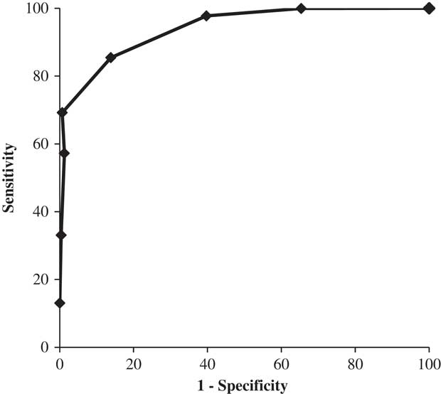
is the number of cows recorded in the hth herd. Next, we constructed the receiver operating characteristic (ROC) curves for SCS values above thresholds going from 0 to 6. Thresholds 0 to 6 span a wide range of SCS values observed in healthy and infected cows and correspond to SCC from 0 to 800 000 cells/ml. A ROC curve is the plot of true-positive rates against false-positive rates for the different threshold values. Thus, a model with high discriminating power has a ROC curve close to the upper left-hand corner of the plot (Uhler, Reference Uhler2009). We also computed the area under the ROC curve using the trapezoid rule (Metz et al., Reference Metz, Herman and Shen1998).
Results and discussion
Description of the data set
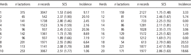
Descriptive data are in Table 1. A total of 29 858 records were collected from 2729 lactations. The incidence of reported cases varied from 0 to 20 cases per 100 cow-years at risk, which is lower than some estimates found in the literature. Indeed, Bradley et al. (Reference Bradley, Leach, Breen, Green and Green2007) and Miltenburg et al. (Reference Miltenburg, de Lange, Crauwels, Bongers, Tielen, Schukken and Elbers1996) reported mean incidence of clinical mastitis ranging from 47% to 71% in England and Wales, and from 13% to 30% in the Netherlands, respectively. In five Holstein herds in the Czech Republic, the overall incidence was 0.68 clinical cases per cow per year, varying from 0.35 to 1.45 cases between farms (Wolfova et al., Reference Wolfova, Stipkova and Wolf2006). Other estimates were nearer to ours with 14.4 cases per 100 cow-years at risk in Uruguay (Gianneechini et al., Reference Gianneechini, Concha, Rivero, Delucci and Moreno Lopez2002) and 14.8 in Norway (Osteras et al., Reference Osteras, Solbu, Refsdal, Roalkvam, Filseth and Minsaas2007). Such differences between countries may be associated with factors such as climate, detection and reporting methods, breed, level of production and management. Another possibility is that not all clinical cases were reported in our study, as suggested by the observation that SCSs were higher in subclinical than clinical mastitis cases. If all clinical cases had been included in the group CM=1 and all subclincal cases in the group CM=2, we would have expected to have an SCS means lower in the group CM=2 than in the group CM=1, assuming that SCS is higher for clinical than subclinical cases.
Descriptive statistics for each herd: number of lactations, number of records, mean for SCS and their standard deviation in parentheses, and incidence (%) of reported clinical case per cow-year at risk

SCS=somatic cell scores.
Means and standard deviations (s.d.) of SCS (averaged over all records) were 1.56 (s.d.=1.10), 4.47 (s.d.=2.43) and 4.78 (s.d.=1.26) for healthy, clinical and subclinical records, respectively. This corresponds roughly to SCC values of 60 000 in healthy, 280 000 in clinical and 340 000 cells/ml in subclinical cases. Underreporting of clinical mastitis has been evidenced, for example, in countries where clinical mastitis cases are routinely registered by farmers, such as Denmark (Klaas et al., Reference Klaas, Enevoldsen, Vaarst and Houe2004) and Sweden (Mork et al., Reference Mork, Lindberg, Alenius, Vagsholm and Egenvall2009). Differences may also be because of the bacterial species responsible for clinical and subclinical cases. Indeed, de Haas et al. (Reference De Haas, Veerkamp, Barkema, Grohn and Schukken2004) showed coliform infections have tendency to be severe with the presence of a short peak in SCC, Staphylococcus aureus infections are less severe (subclinical) and associated with long increased SCC, whereas Streptococcus dysgalactiae and uberis seem not strongly associated with any specific patterns of peaks in SCC.
Comparison between estimated and observed values
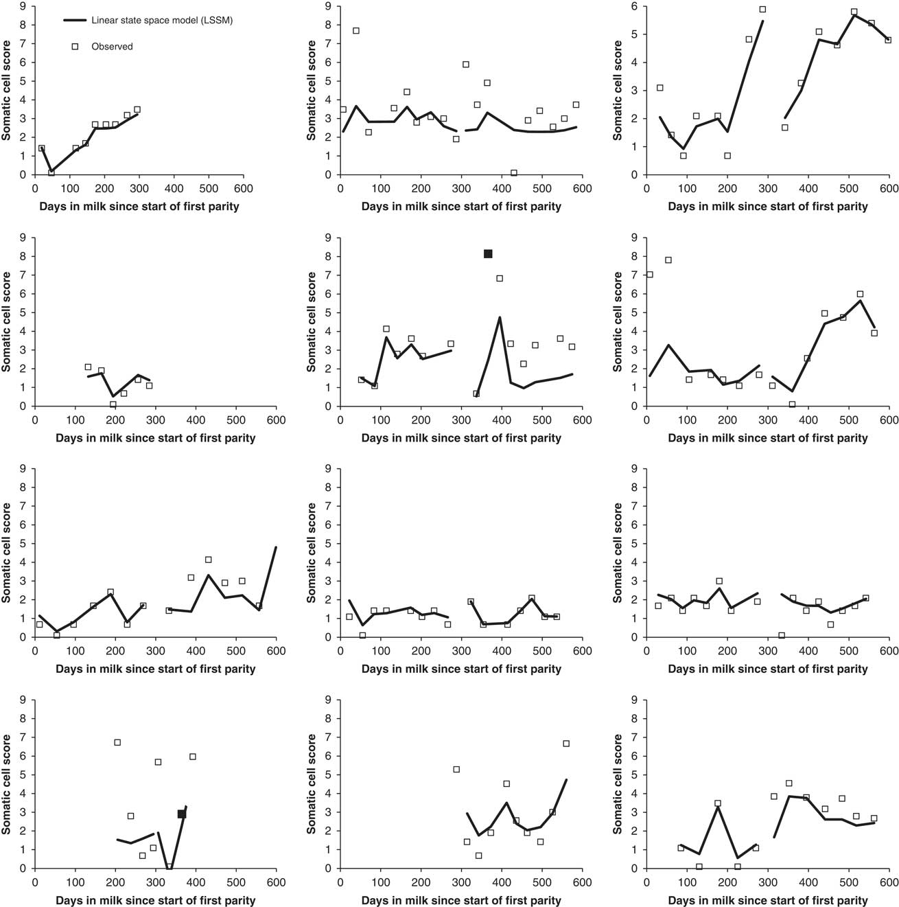
Figure 1 shows observed and estimated SCS lactation curves for several cows taken at random in the data set. One can see that median values of posterior distributions are quite close to observed SCS. Correspondingly, MSEh was very low with a mean of 1.39 over all herds.
Observed and estimated somatic cell score per days in milk since the start of the first parity.

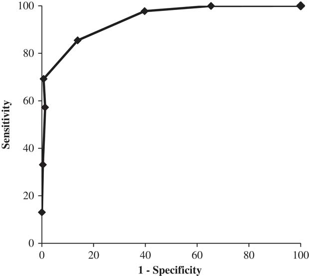
Figure 2 is a ROC plot evaluating the discriminating ability of LSSM in estimating SCS values above thresholds from 0 to 6. The area under the ROC curve is 94.01%, which indicates that LSSM is particularly accurate in correctly classifying records.
Receiver operating characteristic (ROC) plot.
Although it is accurate, the model is very simple and it could be made more realistic by allowing for factors known to have an effect on SCS, being at the cow or herd levels. One such set of factors would be the genetic background of the animals as numerous experiments have identified different genomic regions associated with resistance or susceptibility to mastitis (Pighetti and Elliott, Reference Pighetti and Elliott2011). Management practices (e.g. milking techniques, drying procedures, quality of feed) also influence the prevalence of specific mastitis pathogens and SCS. We could also combine SCS with measurements of biomarkers associated with the disease (Hojsgaard and Friggens, Reference Hojsgaard and Friggens2010).
Parameters of the model
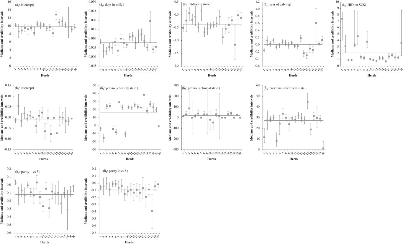
Posterior medians and credibility intervals for all estimated parameters are shown in Figure 3 for each herd, separately. Values for h 2 are shown only for herds in which more than 2.5% of clinical cases were recorded because intervals are quite large in herds where few clinical cases were reported.
Posterior median and corresponding credibility intervals for the estimated model parameters.

When comparing figures for the transition parameters (h 0 to h 3), one may note that h 3 estimates are slightly higher than h 1 estimates and most credibility intervals do not overlap. These estimates (divided by time interval between successive records) may be interpreted as auto-correlations between successive HID (because the transition equations correspond approximately to first-order auto-regressive processes). In our study, correlation between successive HID was higher for a subclinical previous record (h 3) than a healthy previous record (h 1). Stated otherwise, this suggests HID values were linked over time when mastitis was subclinical.
The parameters may also be interpreted in light of our knowledge of the mechanisms of immune/inflammatory response to infection. Therefore, a
4 makes the link between HID and SCS and may represent our uncertainty in measuring HID (as an indicator of defence mechanisms against mastitis pathogens) with SCS. The parameters h
1 to h
3 are linked to the rates of change in leukocyte number under health and infection. In the absence of infection (and if all other factors of HID variation are kept constant), there is an equilibrium where cells enter and leave the udder. In that case, δ
i
t
=δ
i
for all values of t. Then, from the transition equations, we have
 ${ \delta _{i} =\left( {h_{{\rm 0}} HSC_{i}^{{t{\minus}1}} {\plus}h_{{\rm 4}} PAR_{i}^{t} } \right)/\left( {{\rm 1}{\minus}\left( {h_{{\rm 1}} /LAG_{i}^{{t{\minus}{\rm 1}}} } \right)} \right)$
and
 $${ h_{{\rm 1}} =\root\of LAG_{i}^{{t{\minus}{\rm 1}}} $$
because
 ${var(HID_{i} )={\rm 1}=(h_{{\rm 1}} /LAG_{i}^{{t{\minus}{\rm 1}}} )^{{\rm 2}} $
var(HID
i
). When pathogens are present, an extra concentration of leukocytes is recruited in the udder and cells are removed after phagocytosis and killing of pathogens. In such a situation, we may link parameters of the LSSM to parameters of ordinary differential equations (Quach et al., Reference Quach, Brunel and d'Alche-Buc2007), describing the rates at which the cells enter and leave the udder. For example, if cell dynamics is modeled according to a system of equations that reproduce persistent infections (e.g. White et al., Reference White, Schukken, Dogan, Green, Dopfer, Chappell and Medley2010), then a simplified version of the system would be
 $$\delta _{i}^{t} =\delta _{i}^{0} \,e^{{{\minus}h_{3} \,t}} ,$$
with h 3= (g–r), g=rate of influx of cells into the milk in the presence of infection and r=rate of removal. (We chose persistent equations so that the time frame of the LSSM is similar to the timeframe of the ordinary differential equation). This procedure, that is, the formal combination of expert knowledge in the form of dynamic modeling with LSSM on real data, is actually used for estimating disease burden based on surveillance data, often complicated by a tendency for underreporting (e.g. Hooker et al., Reference Hooker, Ellner, Roditi Lde and Earn2011).
In this paper, we propose a simple LSSM to analyze trends in SCS. The model is flexible, it corrects for measurement errors and is relatively easy to implement. It may be extended to account for the dynamics of the response to the infection. Through its hidden variable, it could help in the identification of sub-phenotypes characterized by the same level of expressed genes and decrease the gap between gene and phenotype (Wiggs, Reference Wiggs2010). It could also lead to the identification of disease markers (Morris et al., Reference Morris, Lindgren, Zeggini, Timpson, Frayling, Hattersley and McCarthy2010) and the development of treatment to specific disease symptoms (Hall, Reference Hall2013).
Acknowledgments
This study was supported by the European Research Group EADGENE_S and the Région Wallonne. The authors also thank the OSAM team that collect and store the data.